Seeking Negative Alphas Through Shorting

Abstract

Shorting involves selling stocks that one does not own. Advocates of shorting argue that it is needed to make the financial market a two-way (complete) market in which investors with bearish opinions can participate. To gain from shorting, short sellers hope to buy back the shorted stocks at a lower price. Obtaining ‘negative’ alphas or abnormal returns is thus desirable for short sellers as they imply the underperformance of the stocks and that a profit has been realized. Abnormal returns, according to Fama (1998), are anomalies that tend to disappear when reasonable changes are made to the methodology used to measure them. Diamond and Verrecchia (1987), however, theorize and argue a priori that an unusually large increase in short interest will be followed by a period of negative abnormal returns. Short interest is equal to the number of shorted shares divided by the number of shares available to be shorted. Using daily short interest data for stocks traded on the London Stock Exchange for the period of September 2003 to April 2010, we employ an event study to investigate the effects that follow shorting. Alphas and abnormal returns are measured according to the Market Model (MM), the Capital Asset Pricing Model (CAPM) and the Fama–French Three-factor Model (FF3F), and are estimated using different estimation windows of 60 and 120 days. In all the methodologies under study, we find significant negative alphas following shorting.

Keywords

Shorting short-selling abnormal returns event study market model CAPM Fama-French three-factor model

Introduction

Proponents of shorting argue that shorting is an essential part of price discovery mechanism. Shorting is deemed desirable as it helps complete the financial markets by allowing option market makers to hedge their positions by short selling in cash market (Battalio & Schultz, 2011; Figlewski & Webb, 1993). According to Lamba and Ariff (2006), in a complete financial market, investors must be able to take actions based on their bullish or bearish outlook and Shiller (2003), for example, considers shorting as an essential element of an efficient market. From the short sellers’ perspective, the most important purpose that drives them to short stocks is to earn a negative alpha or an abnormal return. Throughout the short-selling literature, researchers use event studies and calendar time portfolio approaches to show that a negative alpha follows shorting. As shorting is costly, only rational investors with a strong expectation that the stock price will drop will choose to short (Diamond & Verrecchia, 1987). This model argues that short sellers possess significant private information about the stock in question. At a glance, accepting this model is equivalent to admitting that negative alphas are a persistent anomaly, hence rejecting the market efficiency hypothesis. Fama (1998), however, contends that generally apparent anomalies are due to the methodology used and tend to disappear with reasonable changes in technique.

In this study, using the largest daily increases in short interest as a laboratory, we test for information content and compare the mean abnormal returns and alphas produced by alternative models. We also test MacKinlay’s (1997) proposition that the gain from employing multi-factor models in event studies are limited as the marginal explanatory power of any additional factors other than the market factor is very small.

Our empirical results from all 10 of our models are consistent with the analytical work of Diamond and Verrecchia (1987), which predicts negative alphas (and abnormal returns) following the largest increases in short interest in stocks. These anomalies or underperformance of stocks appear to persist for up to 30 days after the event period, for the top percentile of increases in the short interest portfolio. We find significant differences in mean abnormal returns when we compare the top and bottom percentiles of increases in the short interest ratio, suggesting that stronger information content is associated with the largest increases in short interest. When we compare alternative models, estimation windows and weights for the top percentile portfolio, we do not find any significant differences in the mean abnormal returns and alphas, suggesting that short-term anomalies in negative alphas and abnormal returns are not due to the assumed methodology. However, for the portfolio with the smallest increases in short interest, proxied by the bottom percentile portfolio, as suggested by Fama (1998), we do find the choice over whether to use equal or value weights to be an important and relevant issue, as they present conflicting results.

Taken together, the short-term persistent negative alphas derived from different methodologies for the portfolio with the largest increases in short interest may be considered as evidence against the efficient market hypothesis. Investors seeking alpha should find a negative alpha from shorting, in the short term, that is, for up to 30 days following the largest increases in short interest.

The remainder of the article is organized as follows. In the second section, we provide a review of literature. In the third section, we provide objective and rational for study. In the fourth section, we describe the sample frame and methodological considerations. In the fifth section, we report the analysis. In the last section, we offer some concluding remarks.

Review of Literature

Most studies predicting long-term returns with short interest in the United States focus on the level of short interest and define aggregate short interest in a stock as a percentage of the firm’s total shares outstanding. Short interest data in the United States are published on the 20th of every month in the financial press, that is, in the Wall Street Journal, Barron’s National Business and Financial Weekly and The New York Times. Early studies of the information content of short interest in the United States (e.g., Asquith & Meulbroek, 1995; Asquith, Pathak, & Ritter, 2005; Desai, Ramesh, Thiagarajan, & Balachandran, 2002; Jr. Senchack & Starks, 1993) use these market data for their research. Most early studies, with the exception of Senchack and Starks (1993), examine the information content of short interest when the level of short interest hits a certain threshold and use negative monthly Fama–French alphas to indicate the underperformance of the shorted portfolio. Senchack and Starks (1993), however, employ an event study methodology to show negative abnormal returns, following a minimum 100 per cent increase (i.e., at least a doubling) in monthly short interest over the previous month. The recent US studies by Boehmer, Jones and Zhang (2008) and Diether, Lee and Werner (2009), based on daily short sales order flow data, employ Fama–French alphas to show the underperformance of shorted stocks. Blau, Van Ness, Van Ness and Wood (2010) on the other hand use an event study to make inferences about the shorting of stocks, using daily data. As far as Capital Asset Pricing Model (CAPM) is concerned, for the Indian stock market, Basu and Chawla (2010) have concluded that CAPM is not a suitable descriptor of stock prices in India, based on a 2003–2008 sample.

In the United Kingdom, short interest data has been made available to the public by Euroclear UK and Ireland, the UK’s central securities depository, since September 2003, ever since the Financial Services Authority decided to enhance the transparency of short-selling activities. Here, short interest is defined as a percentage of the lendable supply. Au, Doukas and Onayev (2009) use weekly horizon data and employ Fama–French alphas to make inferences about shorting activities in the UK market; they find no significant relationship between high levels of short interest and 52-week stock returns. Mohamad, Jaafar, Hodgkinson and Wells (2013), on the other hand, employ event study on daily short interest data and find that increase in shorting is followed by a period of negative abnormal returns.

Given that previous studies employ either event studies or the calendar time portfolio approach, in this article we use both methodologies and, as stated earlier, consider a total of 10 different models of expected returns. We focus on the largest daily increases and compare them against the smallest daily increases in a short interest portfolio. Here, we define an increase in short interest as a simple increase from one day to the next. We then sort the increases in short interest into percentiles and compare the top and bottom percentiles. We choose simple increases in short interest as a measure of shorting activity for practical reasons. We cannot limit our sample to those that have seen a 100 per cent increase because, unlike Senchack and Starks (1993), we are dealing with high-frequency, daily data. Moreover, it is easier for investors or short sellers to calculate simple increases in short interest from one day to the next, and decide based on that whether to take a risk by shorting the stock.

Objective and Rationale of Study

Fama (1998) argues that stock return anomalies, particularly long-term ones, are difficult to classify as they are plagued by ambiguities and chance. Given that market efficiency must be tested jointly with a model of expected returns, and all models for expected returns are incomplete descriptions of the systematic patterns in average returns during a sample period, tests of market efficiency, arguably, are always contaminated by bad model problems. In addition to the assumed model, the expected returns can be sensitive to the way in which the tests are carried out. Furthermore, equally weighted returns may produce different results to value-weighted returns, and since equal weight portfolio returns give more weight to small stocks, bad model problems can be more severe when inferences are drawn from equally weighted returns.

Our main objective is to examine whether short-term, daily, negative alphas are sensitive to the methodology or assumed model for expected returns. In this article, we study a number of models that have been used in the extant literature to detect a negative alpha in top and bottom percentile portfolios of stocks that experience positive increases in short interest. The main methodologies considered are the event study and calendar time portfolio approaches. Within the event study methodology, we consider the Market Model (MM), the Capital Asset Pricing Model (CAPM) and the Fama–French Three-factor Model (FF3F), while, as calendar time portfolio approaches, we study the Jensen and Fama–French alpha methods. Furthermore, for the event studies we consider two different estimation windows, 60 and 120 days, while for the calendar time portfolios, we consider both equal- and value-weighted returns. To practitioners, this article may have an important implication—if the daily negative alphas are not sensitive to the choice of methodology used, it means that large increases in short interest give a signal to the stock market that some short sellers with private information are shorting the stocks, and afterwards these stocks’ prices might drop. Although such a signal would not be useful in a country like India, where short selling is not allowed, in the United Kingdom, it might come in handy for the investing public looking for an opportunity to make money in the stock market.

The short sellers might argue that they are shorting overvalued stocks, and doing the market a favour by causing their value to drop to equilibrium. Jensen (2005) believes that overvalued equity is a problem when the market price of the stocks is substantially out of line with the fundamental value of the firm, but has never proposed shorting as a solution. Instead, in an earlier paper (Fuller & Jensen, 2002), Jensen advocates for market players refusing to play the earnings management game that leads to the overvaluation of equity.

Previous empirical studies on the information content of short interest are framed with reference to Diamond and Verrecchia’s (1987) private information hypothesis and use either the change or the level of short interest in stocks as a proxy for short-selling activities. Either event studies (Blau et al., 2010; Senchack & Starks, 1993) or the calendar time portfolio approach (Asquith et al., 2005; Desai et al., 2002) are used to show the information content of short interest.

Empirically, the event study methodology has become the standard method of measuring stock returns and providing evidence of stock return anomalies or non-anomalies. A key event study paper by Fama, Fisher, Jensen and Roll (1969), for example, has become a classic paper, having been cited on average about 21 times per year over a 25-year period. Generally, event studies have been widely used for two major reasons: (a) to test the null hypothesis that the market efficiently incorporates information and (b) to examine the impact of some event on the wealth of a firm’s security holders, under the maintained hypothesis that all publicly available information is incorporated in current prices under market efficiency (Binder, 1998).

With respect to event studies, different lengths of estimation windows may yield different sample sizes; in that, the longer is the estimation window, the smaller would be the sample size. The estimation and event windows for the samples must not overlap so as to prevent potential confounding effects from the events on the samples’ abnormal returns. That is, inferences drawn from the event studies may be largely dependent on the sample sizes which in turn are dependent on the choice of length of the estimation windows. We address this issue in the methodological section. Another issue that may affect inferences is cross-sectional dependence in the stock returns sample data. In such circumstances, procedures based on the assumption of independence can yield biased estimates of standard errors and incorrect inferences (Bernard, 1987). The cross-sectional dependency problems may be more likely when the return interval is long, that is, when using quarterly or yearly data. There are several ways to overcome the bias arising from residual cross-correlation. First, researchers can carry out cross-sectional aggregation of the data, which is also known as the calendar time portfolio or Jensen alpha approach. Second, researchers can use a multi-factor version of the MM to measure the dependent variable, as the extra factors incorporated may reduce residual cross-correlation. Previous short-selling studies that opt for cross-sectional aggregation and use a multi-factor model include Asquith et al. (2005), Au et al. (2009), Boehmer et al. (2008), Boehmer, Huszar and Jordan (2010), Desai et al. (2002) and Diether et al. (2009).

On the basis of these issues and concerns, we choose to run a series of event study methodologies and calendar time portfolio approaches and compare the differences in mean abnormal returns between categories so as to ascertain whether the resulting non-zero alphas are due to chance. In our sample, we assume cross-sectional independence in the residuals of the data since increases in short interest are expected to occur randomly.

Methodology

Data Source and Sample Frame

Daily data on short interest is obtained from Euroclear UK and Ireland, while daily data on stock prices, the FTSE350 index prices, market capitalization, dividend yields, market-to-book and price-earnings ratios are sourced from Datastream. As we seek negative alphas through shorting, we confine our sample to stocks that experience positive increases in short interest. We define the short interest ratio as the number of stocks on loan divided by the number of stocks available to be loaned through Euroclear. To engage in shorting, the stocks need to be borrowed (on loan) first. The number of shares on loan thus is a proxy for the number of shorted shares. We also define increases in short interest as simple increases in short interest from one day to the next; thus we begin with 292,623 stocks with daily increases in short interest in our initial sample. We then sort the daily increases into percentiles and take only the top and bottom percentiles as our sample. Naturally, this screening process yields 2,926 observations for each percentile but, after sourcing available market data from Datastream, the number of observations is reduced to 2,255 for the top and 1,777 for the bottom percentile. In Table 1, we report the characteristics of the top and bottom percentile samples. It is worth noting that, for the top percentile portfolio that contains the largest increases in short interest, the increases in short interest range from 1.91 per cent upwards. Meanwhile, for the bottom percentile, the increases in short interest are close to zero. The means and Wilcoxon rank-sum tests shown in Panel C indicate that there is a significant difference between the top and bottom percentiles in terms of market capitalization, market-to-book, price-earnings ratios and dividend yields.

Empirical Model

In this section, we consider several methodologies that can be used to show abnormal performance or alphas following an increase in short interest. The approaches that can be used are event studies and the calendar time portfolio approach.

Event study methodology: MM, estimation period (a) 120 days, from day –120 to day –1 and (b) 60 days, from day –60 to day –1.

The MM, developed by Fama et al. (1969) and later refined by Brown and Warner (1985) for the use of daily data, is a statistical model that relates the return of any given security to the return of the market portfolio. Brown and Warner (1985) find that simple estimation techniques based on ordinary least squares (OLS), with a market index using parametric statistical tests, are well specified under non-normally distributed daily data and in the presence of non-synchronous trading. We estimate the following model over the estimation period: (a) days s = –120 to s = –1 and (b) days s = –60 to s = –1, defined relative to the event date.

Table 1.

Samples’ Descriptive Statistics

Panel A: Top Percentile (N = 2255)	Mean	Median	Std. Dev.	Min	Max
Increase in Short Interest (in %)	3.87	2.92	2.47	1.91	28.31
Market Capitalization (in £ million)	6,906.99	1,951.19	17,297.15	63.13	127,526.70
Market to Book Ratio	3.41	1.98	8.64	0.07	204.19
Price Earnings Ratio	34.24	13.80	445.16	0.40	13197.60
Dividend Yield (in %)	3.54	3.11	5.09	0.00	163.42
Panel B: Bottom Percentile (N =1777)	Mean	Median	Std. Dev.	Min	Max
Increase in Short Interest (in %)	0.00000512	0.000005	0.00000327	0.0000001	0.0000116
Market Capitalization (in £ million)	1,391.92	551.58	4,262.06	56.97	80,162.88
Market to Book Ratio	2.43	1.50	5.12	0.11	178.73
Price Earnings Ratio	56.76	15.50	334.73	2.00	9869.50
Dividend Yield (in %)	2.85	2.57	2.28	0.00	26.41
Panel C: Difference between Top and Bottom Percentile	Mean	p–value		Median	p–value
Increase in Short Interest (in %)	3.87	0.00		2.92	0.00
Market Capitalization (in £ million)	5,515.07	0.00		1,399.61	0.00
Market to Book Ratio	0.98	0.00		0	0.00
Price Earnings Ratio	–22.52	0.09		–1.70	0.00
Dividend Yield (in %)	0.69	0.00		0.54	0.00

Source: Author’s own.

Notes: This table reports descriptive statistics for both the top and bottom percentile portfolios. The top percentile refers to the largest 1% of daily increases in short interest, while the bottom percentile refers to the smallest 1% of daily increases in short interest. An increase in short interest is a simple daily increase from one day to the next. Short interest is expressed as the percentage of the lendable supply of shares that is sold short. Market capitalization is the aggregate value of total outstanding shares in GB pounds (£). Market-to-book is the ratio of the current market value of the shares to the historical book value. Price-earnings is the ratio of the stock price to its per-share earnings. Dividend yield is the current dividend as a percentage of the stock price. N is the number of observations in each portfolio. p-values are for t-tests of the difference in means and the Wilcoxon rank-sum test for the difference in medians.

R_{i s} = {\hat{a}}_{i} + {\hat{b}}_{i} R_{m s} + ε_{i s}

(1)

A R_{i t} = R_{i t} - {\hat{a}}_{i} - {\hat{b}}_{i} R_{m t}

(2)

A A R_{t} = \frac{1}{N} \sum_{i = 1}^{N} A R_{i t}

(3)

C A A R_{t} = \sum_{t = 0}^{t = 30} A A R_{t},

(4)

where R_it denotes the daily logarithmic return for stock i on day t, R_mt denotes the daily logarithmic return on the FTSE350 index, AR_it denotes the daily abnormal return of stock i on day t during the event window (days t = 0 to t = +30, defined again relative to the event date), AAR_t denotes the average daily abnormal return (calculated over all stocks in each sample) on day t and CAAR_t denotes the cumulative average daily abnormal return on day t during the event window. The coefficients ${\hat{a}}_{i}$ and ${\hat{b}}_{i}$ are obtained using the OLS estimation.

Event study methodology: CAPM, estimation period (a) 120 days, from day –120 to day –1 and (b) 60 days, from day –60 to day –1.

The CAPM was established by Sharpe (1964) and Lintner (1965). In this model, the expected returns of a given security are determined by its covariance with the market portfolio. Banz (1981) however finds that returns on small stocks, given their beta, is too high and argues that the CAPM predicts returns that are too low for small firms. We estimate the following model over the estimation period: (a) days s = –120 to s = –1 and (b) days s = –60 to s = –1, defined relative to the event date.

R_{i s} = {\hat{a}}_{i} + {\hat{b}}_{i} (R_{m s} - R_{f s}) + ε_{i s}

(5)

A R_{i t} = R_{i t} - {\hat{a}}_{i} - {\hat{b}}_{i} (R_{m t} - R_{f t})

(6)

A A R_{t} = \frac{1}{N} \sum_{i = 1}^{N} A R_{i t}

(7)

C A A R_{t} = \sum_{t = 0}^{t = 30} A A R_{t},

(8)

where R_it denotes the daily logarithmic return for stock i on day t, R_mt denotes the daily logarithmic return on the FTSE350 index, R_ft denotes average daily return on three-month UK Treasury Bill, for example, on 1 September 2003, where the annualized rate for the UK three-month Treasury Bill is 3.3281 per cent, the average daily return is 3.3281%/365 = 0.0091%. AR_it denotes the daily abnormal return of stock i on day t during the event window (days t = 0 to t = +30, defined again relative to the event date), AAR_t denotes the average daily abnormal return (calculated over all stocks in each sample) on day t and CAAR_t denotes the cumulative average daily abnormal return on day t during the event window. The coefficients ${\hat{a}}_{i}$ and ${\hat{b}}_{i}$ are obtained using the OLS estimation.

Event study methodology: FF3F, estimation period (a) 120 days, from day –120 to day –1 and (b) 60 days, from day –60 to day –1.

In their model, Fama and French (1993) use a three-factor model including a market index, size index and book-to-market index to explain stock returns. The model specifications are as follows:

R_{i s} = {\hat{a}}_{i} + {\hat{b}}_{i} (R_{m s} - R_{f s}) + {\hat{s}}_{i} S M B_{s} + {\hat{h}}_{i} H M L_{s}) + ε_{i s}

(9)

A R_{i t} = R_{i t} - {\hat{a}}_{i} - {\hat{b}}_{i} (R_{m t} - R_{f t}) - {\hat{s}}_{i} S M B_{t} - {\hat{h}}_{i} H M L_{t})

(10)

A A R_{t} = \frac{1}{N} \sum_{i = 1}^{N} A R_{i t}

(11)

C A A R_{t} = \sum_{t = 0}^{t = 30} A A R_{t} .

(12)

We let R_it denote the daily logarithmic return for stock i on day t, R_mt denote the daily logarithmic return on the FTSE350 index and R_ft denote average daily return on three-month UK Treasury Bill. The daily size factor (SMB_t) and value factor (HML_t) are calculated for the UK market following the standard approach described by Fama and French (1993), using data on all listed UK stocks. Our sample for the construction of Fama and French (1996) factors (SMB and HML) uses daily returns data for all UK-listed firms, live and dead, over the period July 2003 to June 2010. We estimate the following model over the estimation period: (a) days s = –120 to s = –1 and (b) days s = –60 to s = –1, defined relative to the event date. The coefficients ${\hat{a}}_{i}, {\hat{b}}_{i}, {\hat{s}}_{i}$ and ${\hat{h}}_{i}$ are obtained using the OLS estimation. We let AR_it denote the daily abnormal return of stock i on day t during the event window (days t = 0 to t = +30, defined again relative to the event date). We let AAR_t denote the average daily abnormal return (calculated over all stocks in each sample) on day t and CAAR_t denote the cumulative average daily abnormal return on day t during the event window.

Jensen Alpha: Equal- and Value-weighted Portfolios

Jensen (1968) examines the performance of mutual fund managers in light of the emerging efficient market hypothesis. The CAPM formula prevailing in 1968 did not permit an evaluation of the fund manager’s performance, so Jensen added a coefficient known as alpha. A positive alpha or intercept signifies overperformance while a negative alpha denotes underperformance of a portfolio compared to a benchmark index. This approach is known as the Jensen alpha approach or the calendar time portfolio approach. The approach was further refined by Jaffe (1974) and Mandelker (1974) and is strongly advocated by Fama (1998). The model specification is as follows:

R_{p t} - R_{f t} = {\hat{a}}_{p} + {\hat{b}}_{p} (R_{m t} - R_{f t}) + ε_{p t},

(13)

where R_pt is the daily calendar time portfolio return on day t, R_mt is the daily return on the FTSE350 index on day t, R_ft is the average risk-free rate, proxied by the UK Treasury Bill rate on day t, and ${\hat{b}}_{p}$ are regression parameters, and ϵ_pt is the error term. The intercept, (Jensen alpha) measures the abnormal performance in the daily return with respect to the CAPM benchmark. In the Jensen alpha method, the alpha is computed using both equal and value weighting of the stocks in the portfolio. Here, we have only two portfolios: the top percentile and the bottom percentile. So, for the Jensen alpha approach, we obtain daily portfolio return series for four calendar time portfolios: (a) equally weighted top percentile portfolio, (b) value-weighted top percentile portfolio, (c) equally weighted bottom percentile portfolio and (d) value-weighted bottom percentile portfolio. Then, the regression is run for all portfolios to find the intercept, ${\hat{a}}_{p}$ (Jensen alpha), for day 0, day 1, day 2, etc. until day 30, following the event. The advantage of the calendar time portfolio approach over the event study methodology is that cross-sectional and serial correlations are not a problem.

Fama–French Alpha: Equal- and Value-weighted Portfolios

The Jensen alpha approach can be further enhanced by incorporating Fama–French factors, in which case the method takes a new name, the Fama–French alpha. The model specification is as follows:

R_{p t} - R_{f t} = {\hat{a}}_{p} + {\hat{b}}_{p} (R_{m t} - R_{f t}) + {\hat{s}}_{p} S M B_{t} + {\hat{h}}_{p} H M L_{t} + ε_{p t} .

(14)

The regression parameters for the Fama–French model are ${\hat{a}}_{p}, {\hat{b}}_{p}, {\hat{s}}_{p}$ and ${\hat{h}}_{p}$ . The three factors ${\hat{b}}_{p}, {\hat{s}}_{p}$ and ${\hat{h}}_{p}$ are zero investment portfolios, representing the excess return of the market (R_m-R_f), the difference between a portfolio of small stocks and a portfolio of big stocks (SMB) and the difference between a portfolio of high book-to-market stocks and a portfolio of low book-to-market stocks, respectively. The intercept ${\hat{a}}_{p}$ (Fama–French alpha) measures the abnormal performance in the daily return with respect to the three-factor benchmark. In the Fama–French alpha method, we again compute alpha using both equal and value weighting of the stocks in the portfolio. Here again, we have just two portfolios: the top percentile and the bottom percentile. So, as with the Jensen alpha approach, we obtain daily portfolio return series for four calendar time portfolios, and run the regression for each portfolio to find the intercept ${\hat{a}}_{p}$ from day 0 to day 30, following the event.

Sample Selection Due to Different Estimation Periods in the Event Study

In the event study, the analysis of aggregated abnormal returns requires an assumption that the event windows of the included securities do not overlap in calendar time. This assumption specifically allows the calculation of the variance of the aggregated sample of cumulative abnormal returns, without concern about covariances across securities, as they are zero (MacKinlay, 1997). As mentioned earlier, the estimation and event windows for the included securities are also assumed not to overlap, in order to prevent potential confounding effects from the events on stocks returns. There is no clear-cut rule as to what is the best length of estimation window in an event study. The trade-off is that the longer is the estimation window, the fewer samples can be included and this may result in a test with less power to show non-zero abnormal returns.

In Figure 1, we find that when the estimation period is lengthened from 60 to 120 days, the number of observations in the top percentile portfolio reduces considerably from 1,247 to 1,021, while the number in the bottom percentile portfolio falls from 987 to 788. The venn diagrams show that the number of observations common to both sizes of estimation window are 971 and 741 for the top and bottom percentile portfolios, respectively. The number of observations that only appear under one or the other of the estimation windows is 326 (276 + 50) and 293 (246 + 47) for the top and bottom percentile portfolios, respectively. The aim here is to test whether the difference in the number of observations, as a result of the difference in estimation periods, will result in a significant difference in the mean abnormal return.

Analysis

Cumulative Abnormal Returns and Alphas for All Models

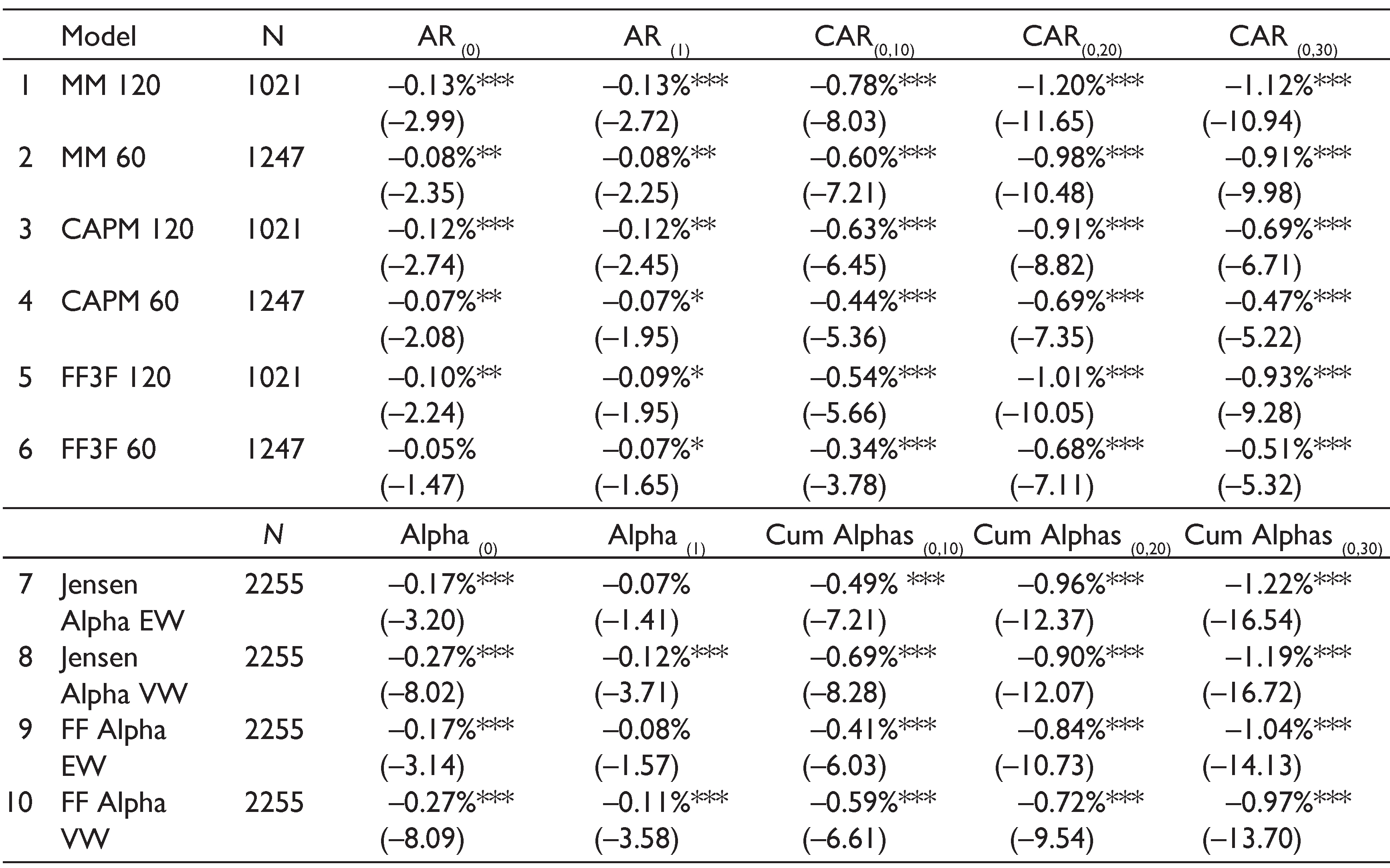
In Table 2, we report the abnormal returns and alphas for day 0 and day 1, as well as cumulative abnormal returns and cumulative alphas for day 0, 1, (0, 10), (0, 20) and (0, 30), for all models, for the top percentile portfolio. The models are the MM with 120-day estimation window (MM 120), the MM with 60-day estimation window (MM 60), CAPM with 120-day estimation window (CAPM 120), CAPM with 60-day estimation window (CAPM 60), FF3F with 120-day estimation window (FF3F 120), FF3F with 60-day estimation window (FF3F 60), Jensen alpha equal weighted (Jensen alpha EW), Jensen alpha value weighted (Jensen alpha VW), Fama–French alpha equal weighted (FF alpha EW) and Fama–French alpha value weighted (FF alpha VW).

Generally speaking, all models show underperformance following the largest increases in short interest, proxied by top percentile increases in short interest. When abnormal returns and alphas are cumulated over multi-day intervals, all models show significant underperformance, with the Jensen alpha equally weighted portfolio showing the biggest underperformance of 1.22 per cent for the 30 trading days, following the largest increases in short interest. However, for the 20 and 10 trading day intervals, (0, 20) and (0, 10), MM 120 yields the greatest underperformance of 1.20 per cent and 0.78 per cent, respectively. The test statistic for multi-day interval cumulative alphas is the ratio of cumulative alphas to their estimated standard deviation, and is given by:

\sum_{t = 0}^{T} \frac{C A A R_{t}}{\sqrt{\sum_{t = 0}^{T} {\hat{S}}^{2} (C A A R_{t})},}

(15)

\begin{matrix} w h e r e \end{matrix} \hat{S} (C A A R_{t}) = \frac{1}{N - 1} \sum_{i = 1}^{N} {(C A R_{i} - C A A R_{t})}^{2}

C A R_{i} = \frac{1}{N} \sum_{t = t_{1}}^{t_{2}} A R_{i t} .

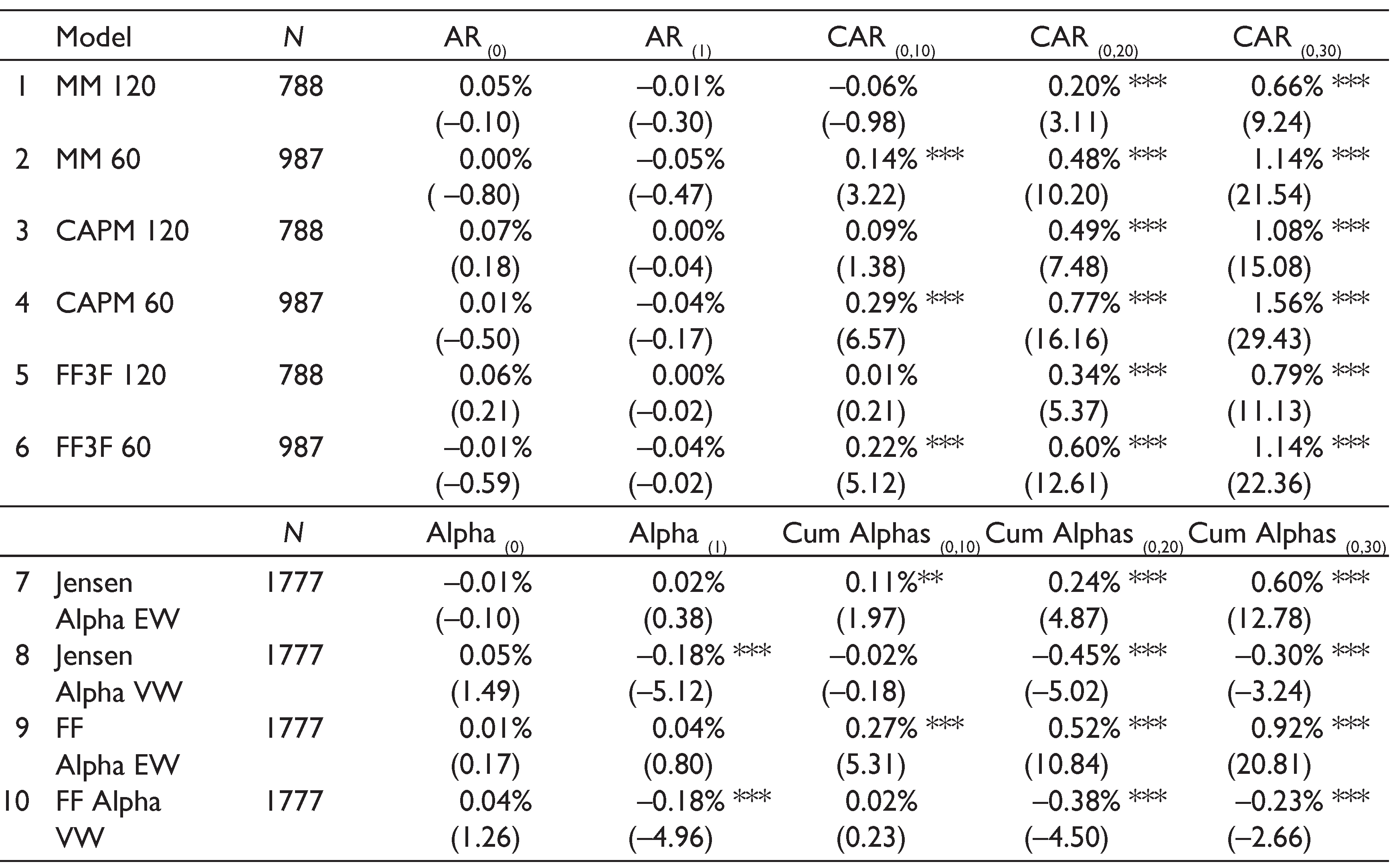
In Table 3, we present the cumulative abnormal returns and alphas for all models, for the bottom percentile portfolio. Unlike the top percentile, the bottom percentile yields some conflicting results. For multi-day intervals, CAPM 60 with a (0, 30) interval shows the biggest overperformance of 1.56 per cent, whereas cumulative Jensen alphas on value-weighted portfolios for the (0, 20) interval yields the biggest underperformance of 0.45 per cent.

By and large, here, all event study models show very similar results but, for the calendar time portfolio approach, the results of the equally weighted method appear to contradict those of the value-weighted method. The equally weighted portfolios tend to show positive cumulative alphas, while the value-weighted portfolios tend to show negative cumulative alphas. It appears that the bottom percentile portfolio is dominated by large capitalization stocks, which explains the negative cumulative alphas obtained using value-weighted portfolios.

Table 2.

Cumulative Abnormal Returns and Alphas for Top Percentile Portfolio

	Model	N	AR₍₀₎	AR ₍₁₎	CAR_(0,10)	CAR_(0,20)	CAR _(0,30)
1	MM 120	1021	–0.13%***	–0.13%***	–0.78%***	–1.20%***	–1.12%***
			(–2.99)	(–2.72)	(–8.03)	(–11.65)	(–10.94)
2	MM 60	1247	–0.08%**	–0.08%**	–0.60%***	–0.98%***	–0.91%***
			(–2.35)	(–2.25)	(–7.21)	(–10.48)	(–9.98)
3	CAPM 120	1021	–0.12%***	–0.12%**	–0.63%***	–0.91%***	–0.69%***
			(–2.74)	(–2.45)	(–6.45)	(–8.82)	(–6.71)
4	CAPM 60	1247	–0.07%**	–0.07%*	–0.44%***	–0.69%***	–0.47%***
			(–2.08)	(–1.95)	(–5.36)	(–7.35)	(–5.22)
5	FF3F 120	1021	–0.10%**	–0.09%*	–0.54%***	–1.01%***	–0.93%***
			(–2.24)	(–1.95)	(–5.66)	(–10.05)	(–9.28)
6	FF3F 60	1247	–0.05%	–0.07%*	–0.34%***	–0.68%***	–0.51%***
			(–1.47)	(–1.65)	(–3.78)	(–7.11)	(–5.32)
		N	Alpha ₍₀₎	Alpha ₍₁₎	Cum Alphas _(0,10)	Cum Alphas _(0,20)	Cum Alphas _(0,30)
7	Jensen Alpha EW	2255	–0.17%***	–0.07%	–0.49% ***	–0.96%***	–1.22%***
			(–3.20)	(–1.41)	(–7.21)	(–12.37)	(–16.54)
8	Jensen Alpha VW	2255	–0.27%***	–0.12%***	–0.69%***	–0.90%***	–1.19%***
			(–8.02)	(–3.71)	(–8.28)	(–12.07)	(–16.72)
9	FF Alpha EW	2255	–0.17%***	–0.08%	–0.41%***	–0.84%***	–1.04%***
			(–3.14)	(–1.57)	(–6.03)	(–10.73)	(–14.13)
10	FF Alpha VW	2255	–0.27%***	–0.11%***	–0.59%***	–0.72%***	–0.97%***
			(–8.09)	(–3.58)	(–6.61)	(–9.54)	(–13.70)

Source: Author’s own.

Notes: This table reports the results of a multi-day analysis of the event study and calendar time portfolio approaches for the top percentile of increases in the short interest, for the period from September 2003 to April 2010. Abnormal returns and alphas are measured for the models given below, and cumulated for 10, 20 and 30 days, following the largest increases in short interest. 120 and 60 refer to 120-day and 60-day estimation periods, EW and VW refer to equal and value weightings, FF refers to Fama–French, and N is the number of observations. Following Brown and Warner (1985), we construct multi-day test statistics to show significance. *, ** and *** denote statistical significance at 10%, 5% and 1%, respectively. We report the t-statistics in parentheses.

Cumulative Abnormal Returns: Top Versus Bottom Percentile Portfolio

In Figure 2, we chart the cumulative abnormal returns for all event study models, for both top and bottom percentile portfolios, and compare them side by side. We find a striking difference between the two portfolios. For the top percentile portfolio, we find positive cumulative abnormal returns for all models, but for the bottom percentile portfolio, we find negative cumulative abnormal returns for all models. Second, over a period of 30 days following the largest increases in short interest, the MM 120 model shows the greatest underperformance while the CAPM 60 model shows the least underperformance. Third, over a period of 30 days following the smallest increases in short interest, the MM 120 shows the least overperformance, while the CAPM 60 shows the greatest overperformance.

Table 3.

Cumulative Abnormal Returns and Alphas for Bottom Percentile Portfolio

	Model	N	AR₍₀₎	AR ₍₁₎	CAR _(0,10)	CAR _(0,20)	CAR _(0,30)
1	MM 120	788	0.05%	–0.01%	–0.06%	0.20% ***	0.66% ***
			(–0.10)	(–0.30)	(–0.98)	(3.11)	(9.24)
2	MM 60	987	0.00%	–0.05%	0.14% ***	0.48% ***	1.14% ***
			( –0.80)	(–0.47)	(3.22)	(10.20)	(21.54)
3	CAPM 120	788	0.07%	0.00%	0.09%	0.49% ***	1.08% ***
			(0.18)	(–0.04)	(1.38)	(7.48)	(15.08)
4	CAPM 60	987	0.01%	–0.04%	0.29% ***	0.77% ***	1.56% ***
			(–0.50)	(–0.17)	(6.57)	(16.16)	(29.43)
5	FF3F 120	788	0.06%	0.00%	0.01%	0.34% ***	0.79% ***
			(0.21)	(–0.02)	(0.21)	(5.37)	(11.13)
6	FF3F 60	987	–0.01%	–0.04%	0.22% ***	0.60% ***	1.14% ***
			(–0.59)	(–0.02)	(5.12)	(12.61)	(22.36)
		N	Alpha ₍₀₎	Alpha ₍₁₎	Cum Alphas _(0,10)	Cum Alphas _(0,20)	Cum Alphas _(0,30)
7	Jensen Alpha EW	1777	–0.01%	0.02%	0.11%**	0.24% ***	0.60% ***
			(–0.10)	(0.38)	(1.97)	(4.87)	(12.78)
8	Jensen Alpha VW	1777	0.05%	–0.18% ***	–0.02%	–0.45% ***	–0.30% ***
			(1.49)	(–5.12)	(–0.18)	(–5.02)	(–3.24)
9	FF Alpha EW	1777	0.01%	0.04%	0.27% ***	0.52% ***	0.92% ***
			(0.17)	(0.80)	(5.31)	(10.84)	(20.81)
10	FF Alpha VW	1777	0.04%	–0.18% ***	0.02%	–0.38% ***	–0.23% ***
			(1.26)	(–4.96)	(0.23)	(–4.50)	(–2.66)

Source: Author’s own.

Notes: This table reports the results of a multi-day analysis of the event study and calendar time portfolio approaches for the portfolio made up of the bottom percentile of increases in short interest, for the period from September 2003 to April 2010. Abnormal returns and alphas are measured for the various models, and cumulated for 10, 20 and 30 days, following the smallest increases in short interest. Following Brown and Warner (1985), we construct multi-day test statistics to show significance. *, ** and *** denote statistical significance at 10%, 5% and 1%, respectively. We report the t-statistics in parentheses.

Cumulative Alphas: Top Versus Bottom Percentile Portfolio

We present the cumulative alphas for the top and bottom percentile portfolios in Figure 3. For the top percentile portfolio, all models—Jensen alpha EW, Jensen alpha VW, FF alpha EW and FF alpha VW—show a very similar pattern of underperformance, with Jensen alpha EW showing the greatest underperformance. In the bottom percentile portfolio, the pattern is not consistent, however. While the equally weighted portfolios for both Jensen and Fama–French alpha show overperformance, the value-weighted portfolios show the opposite: underperformance. Again, these negative cumulative alphas in the value-weighted portfolios may suggest that large capitalization stocks dominate the bottom percentile portfolio.

Comparison of Mean Abnormal Returns Between Categories

We compare mean abnormal returns between categories over several event windows in Table 4 and report the differences in mean abnormal returns in the upper row and the t-statistics of the differences in parentheses.

Top Versus Bottom Percentile (Largest Versus Smallest Increases in Short Interest)

In Panel A of Table 4, we compare and report the differences in mean abnormal returns between the top and bottom percentiles, while holding methodology and number of estimation days constant. We find that, by and large, mean abnormal returns between the top and bottom percentiles are significantly different, particularly for long event windows, that is, (0, 20) and (0, 30). This result specifically shows that the mean abnormal returns for stocks that experience the largest increases in short interest are significantly more negative than those for stocks that experience the smallest increases in short interest, thus providing empirical evidence to support Diamond and Verrecchia’s (1987) hypothesis that an unusually large increase in short interest is bad news.

120 Versus 60-day Estimation Period

In Panel B of Table 4, we present the differences in mean abnormal returns between the 120- and 60-day estimation windows, while holding methodology and top or bottom portfolio constant. We do not find any significant differences in the mean abnormal returns between the two estimation windows, for any model or event window. Recall that earlier, in Figure 1, we presented the sample sizes for 120- and 60-day estimation windows. The number of common observations are 971 and 741, while the unique observations are 326 (276 + 50) and 293 (246 + 47) for the top and bottom percentile portfolios, respectively. It appears that the differences in mean abnormal returns in the unique observations resulting from different estimation windows are not large enough to influence the common samples. This finding may imply that the choice of estimation window, at least between 120 and 60 days, will not significantly influence the results, and that it cannot be used to ‘create’ a desired result.

Table 4.

Comparison of Mean Abnormal Returns

Panel A (Top Percentile vs Bottom Percentile)
EventWindow	MM120 TopvsMM120 Bottom	CAPM120 TopvsCAPM120 Bottom	FF3F120 TopvsFF3F120 Bottom	MM60 TopvsMM60 Bottom	CAPM60 TopvsCAPM60 Bottom	FF3F60 TopvsFF3F60 Bottom
(0, +1)	–0.15%**	–0.15%**	–0.13%*	–0.06%	–0.06%	–0.03%
	(–1.99)	(–1.99)	(–1.65)	(–0.81)	(–0.80)	(–0.49)
(0, +10)	–0.07%**	–0.06%**	–0.05%	–0.07%**	–0.07%**	–0.05%*
	(–2.07)	(–2.06)	(–1.59)	(–2.35)	(–2.33)	(–1.78)
(0, +20)	–0.07%***	–0.07%***	–0.06%***	–0.07%***	–0.07%***	–0.06%***
	(–2.78)	(–2.76)	(–2.69)	(–3.19)	(–3.17)	(–2.82)
(0, +30)	–0.06%***	–0.06%***	–0.06%***	–0.07%***	–0.07%***	–0.05%***
	(–2.95)	(–2.92)	(–2.85)	(–3.71)	(–3.68)	(–3.00)
Panel B (120 vs 60 Days Estimation Period)
EventWindow	MM120 TopvsMM60 Top	CAPM120 TopvsCAPM60 Top	FF3F120 TopvsFF3F60 Top	MM120 BottomvsMM60 Bottom	CAPM120 BottomvsCAPM60 Bottom	FF3F120 BottomvsFF3F60 Bottom
(0, +1)	–0.05%	–0.05%	–0.04%	0.05%	0.05%	0.06%
	(–0.69)	(–0.69)	(–0.52)	(0.65)	(0.65)	(0.74)
(0, +10)	–0.02%	–0.02%	–0.02%	–0.02%	–0.02%	–0.02%
	(–0.56)	(–0.56)	(–0.61)	(–0.61)	(–0.61)	(–0.61)
(0, +20)	–0.01%	–0.01%	–0.02%	–0.01%	–0.01%	–0.01%
	(–0.45)	(–0.45)	(–0.66)	(–0.64)	(–0.64)	(–0.59)
(0, +30)	–0.01%	–0.01%	–0.01%	–0.02%	–0.02%	–0.01%
	(–0.35)	(–0.35)	(–0.70)	(–0.93)	(–0.93)	(–0.69)
Panel C (Comparison between Methodologies for Top Percentile)
EventWindow	MM120 TopvsCAPM120 Top	MM120 TopvsFF3F120 Top	CAPM120 TopvsFF3F120 Top	MM60 TopvsCAPM60 Top	MM60 TopvsFF3F60 Top	CAPM60 TopvsFF3F60 Top
(0, +1)	–0.01%	–0.04%	–0.02%	–0.01%	–0.02%	–0.01%
	(–0.19)	(–0.49)	(–0.30)	(–0.20)	(–0.36)	(–0.15)
(0, +10)	–0.01%	–0.02%	–0.01%	–0.01%	–0.02%	–0.01%
	(–0.46)	(–0.73)	(–0.27)	(–0.49)	(–0.83)	(–0.33)
(0, +20)	–0.01%	–0.01%	0.00%	–0.01%	–0.01%	0.00%
	(–0.56)	(–0.38)	(0.19)	(–0.61)	(–0.63)	(–0.01)
(0, +30)	–0.01%	–0.01%	0.01%	–0.01%	–0.01%	0.00%
	(–0.69)	(–0.31)	(0.39)	(–0.75)	(–0.69)	(0.06)

Source: Author’s own.

Notes: This table reports the differences in mean abnormal returns between categories over several event windows for the period from September 2003 to April 2010. Abnormal returns are measured according to each model below. The number of observations (N) for the 120-day and 60-day estimation periods, and top and bottom percentiles are 1,021, 1,247, 788 and 987, respectively. We construct a two-sample t-test to show the significances of the differences and report the t-statistics in parentheses. *, ** and *** denote statistical significance at 10%, 5% and 1%, respectively.

Comparison Between Event Study Methodologies

In Panel C of Table 4, we show the differences in mean abnormal returns between the event study methodologies, while holding the estimation window and top or bottom percentile portfolio constant. Here, we compare the MM with the CAPM, the MM with the FF3F and the CAPM with the FF3F. Surprisingly, we do not find any significant differences in the mean abnormal returns between methodologies for any of these models and using any event windows. Our finding is in line with MacKinlay (1997), who argues that the gains from employing multi-factor models for event studies are limited because the marginal explanatory power of additional factors other than the market factor is small. A multi-factor model, according to MacKinlay (1997), can be considered if the sample firms have common characteristics; hence, the variance reduction in the abnormal returns will be the greatest.

Comparison of Alphas Between Categories

We compare alphas between categories over several event windows in Table 5, reporting the differences in the mean alphas in the upper row and the t-statistics of the differences in parentheses.

Equal Versus Value Weighted

In Panel A of Table 5, we compare and report the differences in mean alphas between equal and value-weighted portfolios, while holding methodology constant for several holding periods. Generally, for the top percentile portfolio, there is no difference in alphas regardless of whether we use equal or value weighting. The difference does become apparent for the bottom percentile portfolio, though, particularly for the Fama–French alpha in the longer holding periods: (0, 20) and (0, 30). This result is not surprising, as we stated earlier that the composition of the bottom percentile portfolio may be dominated by large capitalization stocks. Boehmer et al. (2010) argue that, although value weighting is preferable as it reflects the average investor, it does not reflect the investor’s net short position, which is zero in all stocks at all times. It is therefore not clear that the value weighting method is superior to equal weights in examining the performance of shorted stocks.

Comparison Between Calendar Time Portfolio Approaches

In Panel B of Table 5, we present the differences in the mean alphas of the calendar time portfolio approaches, while holding weights and top or bottom percentile portfolios constant. In this table, we compare the Jensen and Fama–French alpha approaches over several holding periods. Holding the weights constant, we do not find any significant difference in the mean alphas of the Jensen and Fama–French approaches in any of the holding periods. This result may suggest that the gain from employing a multi-factor model for the calendar time portfolio approach may be limited, due to the very small marginal explanatory power of factors other than the market factor.

Table 5.

Comparison of Alphas

Panel A (Equal vs Value Weighted)
HoldingPeriod	Jensen Alpha Top EWvsJensen Alpha Top VW	Fama-French Alpha Top EWvsFama–French Alpha Top VW	Jensen Alpha Bottom EWvsJensen Alpha Bottom VW	Fama-French Alpha Bottom EWvsFama–French Alpha Bottom VW
(0, +1)	0.07%	0.07%	0.07%	0.09%
	(0.80)	(0.76)	(0.62)	(0.84)
(0, +10)	0.01%	0.01%	0.01%	0.02%
	(0.31)	(0.24)	(0.33)	(0.70)
(0, +20)	0.00%	–0.01%	0.03%	0.04%*
	(–0.13)	(–0.24)	(1.47)	(2.02)
(0, +30)	0.00%	0.00%	0.03%	0.04%**
	(–0.05)	(–0.13)	(1.56)	(2.11)
Panel B (Comparison between Methodologies holding Weight Constant)
HoldingPeriod	Jensen Alpha Top EWvsFama–French Alpha Top EW	Jensen Alpha Top VWvsFama–French Alpha Top VW	Jensen Alpha Bottom EWvsFama–French Alpha Bottom EW	Jensen Alpha Bottom VWvsFama–French Alpha Bottom VW
(0, +1)	0.00%	0.00%	–0.02%	0.00%
	(0.03)	(–0.02)	(–0.96)	(0.01)
(0, +10)	–0.01%	–0.01%	–0.01%	0.00%
	(–0.21)	(–0.25)	(–0.64)	(–0.09)
(0, +20)	–0.01%	–0.01%	–0.01%	0.00%
	(–0.27)	(–0.39)	(–0.88)	(–0.13)
(0, +30)	–0.01%	–0.01%	–0.01%	0.00%
	(–0.30)	(–0.40)	(–0.88)	(–0.09)

Source: Author’s own.

Notes: This table reports the difference in mean alphas between categories over several holding periods for the period from September 2003 to April 2010. Alphas are measured using either the Jensen or Fama–French alpha method. The number of observations (N) in the top and bottom percentiles are 2,255 and 1,777, respectively. We construct a two-sample t-test to show the significance of the differences and report the t-statistics in parentheses. *, ** and *** denote statistical significance at 10%, 5% and 1%, respectively.

Conclusion

In this article, we compare the abnormal returns and alphas of several portfolios following the shorting of stocks. Specifically, we compare across different categories: (a) top and bottom percentile portfolios, (b) 120- and 60-day estimation windows, (c) different models of event studies, (d) equal and value weightings and (e) different models of the calendar time portfolio approach. In all categories, we test for differences in mean abnormal returns and alphas for all models in several event windows and holding periods. For the event study methodology, the difference between the top and bottom percentiles is extremely significant. However, the differences between different estimation windows and choices of model for the event study approach are very marginal and insignificant. Similarly, for the calendar time portfolio approach, we find significant differences between the results of using equal and value weightings over long holding periods, but no significant differences resulting from the choice of model, that is, between the Jensen and Fama–French alpha approaches.

Our evidence is in line with MacKinlay’s (1997) argument that the gains from employing multi-factor models in event studies are limited as the marginal explanatory power of factors other than the market factor is very small. For event studies, the choices of methodology and estimation window appear to be immaterial. For the calendar time portfolio approach, however, the choice of weighting approach appears very important, as equal and value weightings can yield opposing results. We agree with Boehmer et al. (2010) that, while value weightings may not be superior to equal weightings when studying the performance of shorted stocks, the potentially conflicting results may require disclosure of the results of both.

Our findings have several important implications. First, despite Fama’s (1998) strong rebuttal, claiming apparent anomalies are methodological illusions, we find that shorting anomalies persist in all the models under study, particularly with respect to the top percentile with the largest increases in short interest. Second, from an empirical point of view, this exercise provides supporting evidence for Diamond and Verrecchia’s (1987) hypothesis that unusually large increases in short interest are associated with periods of negative alphas. Third, our evidence shows that UK short sellers may have the chance to strike negative alphas if the increases in short interest are 1.91 per cent or more. Investors seeking negative alphas can find them through shorting. Last but not least, allowing shorting in the stock market may be one solution for preventing overvalued equity. Future research could be undertaken to investigate whether these negative alpha shorted stocks owners have ever played the earnings management game that results in overvaluation of stocks.

Footnotes

Acknowledgements

The author is grateful the anonymous referees of the journal for their useful suggestions to improve the quality of the article. Usual disclaimers apply.

References

Asquith

& Meulbroek

(1995). An empirical investigation of short interest. Boston, MA: Division of Research, Harvard Business School.

Asquith

Pathak

P.A.

& Ritter

J.R.

(2005). Short interest, institutional ownership, and stock returns. Journal of Financial Economics, 78(2), 243–276.

A.S.

Doukas

J.A.

& Onayev

(2009). Daily short interest, idiosyncratic risk, and stock returns. Journal of Financial Markets, 12(2), 290–316.

Banz

R.W.

(1981). The relationship between return and market value of common stocks. Journal of Financial Economics, 9(1), 3–18.

Basu

& Chawla

(2010). An empirical test of CAPM—The case of Indian stock market. Global Business Review, 11(2), 209–220.

Battalio

& Schultz

(2011). Regulatory uncertainty and market liquidity: The 2008 short sale ban’s impact on equity option markets. The Journal of Finance, 66(6), 2013–2053.

Bernard

V.L.

(1987). Cross-sectional dependence and problems in inference in market-based accounting research. Journal of Accounting Research, 25(1), 1–48.

Binder

(1998). The event study methodology since 1969. Review of Quantitative Finance and Accounting, 11(2), 111–137.

Blau

B.M.

Van Ness

& Wood

(2010). Short selling during extreme market movements. Journal of Trading, 5(4), 14–27.

10.

Boehmer

Huszar

Z.R.

& Jordan

B.D.

(2010). The good news in short interest. Journal of Financial Economics, 96(1), 80–97.

11.

Boehmer

Jones

C.M.

& Zhang

(2008). Which shorts are informed? The Journal of Finance, 63(2), 491–527.

12.

Brown

S.J.

& Warner

J.B.

(1985). Using daily stock returns: The case of event studies. Journal of Financial Economics, 14(1), 3–31.

13.

Desai

Ramesh

Thiagarajan

S.R.

& Balachandran

B.V.

(2002). An investigation of the informational role of short interest in the Nasdaq market. The Journal of Finance, 57(5), 2263–2287.

14.

Diamond

D.W.

& Verrecchia

R.E.

(1987). Constraints on short-selling and asset price adjustment to private information. Journal of Financial Economics, 18(2), 277–311.

15.

Diether

K.B.

Lee

& Werner

I.M.

(2009). Short-sale strategies and return predictability. Review of Financial Studies, 22(2), 575–607.

16.

Fama

E.F.

(1998). Market efficiency, long-term returns, and behavioral finance. Journal of Financial Economics, 49(3), 283–306.

17.

Fama

E.F.

& French

K.R.

(1993). Common risk factors in the returns on stocks and bonds. Journal of Financial Economics, 33(1), 3–56.

18.

Fama

E.F.

& French

K.R.

(1996). Multifactor explanations of asset pricing anomalies. The Journal of Finance, 51(1), 55–84.

19.

Fama

E.F.

Fisher

Jensen

& Roll

(1969). The adjustment of stock prices to new information. International Economic Review, 10(1), 1–21.

20.

Figlewski

& Webb

G.P.

(1993). Options, short sales, and market completeness. Journal of Finance, 48(2), 761–777.

21.

Fuller

& Jensen

M.C.

(2002). Just say no to Wall Street: Putting a stop to the earnings game. Journal of Applied Corporate Finance, 14(4), 41–46.

22.

Jaffe

J.F.

(1974). Special information and insider trading. The Journal of Business, 47(3), 410–428.

23.

Jensen

M.C.

(1968). The performance of mutual funds in the period 1945–1964. The Journal of Finance, 23(2), 389–416.

24.

Jensen

M.C.

(2005). Agency costs of overvalued equity. Financial Management, 34(1), 5–19.

25.

Lamba

A.S.

& Ariff

(2006). Short selling restrictions and market completeness: The Malaysian experience. Applied Financial Economics, 16(5), 385–393.

26.

Lintner

(1965). The valuation of risk assets and the selection of risky investments in stock portfolios and capital budgets. Review of Economics and Statistics, 47(1), 13–37.

27.

MacKinlay

A.C.

(1997). Event studies in economics and finance. Journal of Economic Literature, 35(1), 13–39.

28.

Mandelker

(1974). Risk and return: The case of merging firms. Journal of Financial Economics, 1(4), 303–335.

29.

Mohamad

Jaafar

Hodgkinson

& Wells

(2013). Short selling and stock returns: Evidence from the UK. The British Accounting Review, 45(2), 125–137.

30.

Senchack

A.J.

Jr & Starks

L.T.

(1993). Short-sale restrictions and market reaction to short-interest announcements. The Journal of Financial and Quantitative Analysis, 28(2), 177–194.

31.

Sharpe

W.F.

(1964). Capital asset prices: A theory of market equilibrium under conditions of risk. Journal of Finance, 19(3), 425–442.

32.

Shiller

R.J.

(2003). From efficient markets theory to behavioral finance. Journal of Economic Perspectives, 17(1), 83–104.