
Abstract
One might claim that a researcher can estimate the impact of exchange rate volatility on exports, considering the regime shifts. Otherwise, the relevant estimation output might be biased. This article examines the possible impact of exchange rate volatility on export in Turkey by employing the monthly data for the period 2003M1 and 2015M4. To this end, the article develops a model based on the demand for the traditional long-term aggregate export in which the influences of volatility of exchange rate, domestic income level, foreign income level and ratio of foreign price to domestic price on the real export level are observed. The article (a) first reviews the relevant literature evidence, (b) then follows the preliminary methodologies of unit root test with structural breaks or break point tests through regime shifts (c) and later, estimates the cointegration coefficients of Hatemi-J regime switching models, dynamic ordinary least square (DOLS) and fully modified ordinary least square models to understand the behaviour of Turkish export in detail.
The motivation of this article lies in two points. First, the article considers mainly the effect of exchange rate volatility on Turkish export by observing the possible existence of structural breaks and/or regime shifts. Second, the article follows both (C/S) regime switching model and (C/T) regime switching model, where (C/S) represents the model in which regime changes are observed in constant and in all regressors and where (C/T) denotes the model in which the regime shifts are estimated in constant along with trend of the Turkish export equation. The regime switching model (C/S) exhibits the positive effects of volatility, domestic income and price ratio (W/Tr) and negative impact of World income on Turkish export. The DOLS estimations support the (C/S) model outputs except the sign of price ratio. Eventually the article reveals that (a) the Turkish exporters appear to be risk lovers rather than risk-averse and (b) Turkish export should give more weight to MENA countries.
Keywords
Introduction
Exchange rates have started to fluctuate significantly and unexpectedly since the collapse of Bretton Woods system of fixed exchange rates. The exchange rate volatility might stem from the changes in terms of trade, trade openness, economic growth, money supply, inflation rate (Raza & Afshan, 2017) or volatility of other countries’ exchange rates (Kumar, 2014). The unforeseen fluctuations in exchange rates (exchange rates uncertainty called volatility) cause important changes on foreign trade dynamics, economic policies and variables such as the interest rate, inflation rate, domestic investment and FDI. However, the first and direct impact caused by the exchange rate volatility appears on international trade (Serenis & Tsounis, 2013) due to the fact that it exposes the trade to some uncertainties related with sales and profitability (McKenzie, 1999). The impact of the volatilities on trade volumes might be negative or positive. The sign of the impact depends on some assumptions or some facts about countries, such as structure of the economy, presence of future or forward markets and hedging instruments, trader’s risk preferences and so on (Auboin & Ruta 2013; Bahmani-Oskooee & Hegerty, 2007). Moreover, Sercu and Uppal (2003) show that the sign of the effect of the volatility may change depending on the underlying source of fluctuations.
Theoretical analyses of the connection between higher exchange rate volatility and international trade activities have been carried out by Hooper and Kohlhagen (1978). They claim that greater exchange rate volatility leads to greater cost for risk-averse dealers and to less foreign trade. This occurs because the exchange rate is determined at the epoch of the trade contract, but payment is not done until the future submittal actually comes true. If alteration in exchange rate grows unpredictably, this brings about uncertainty about the profits and, as a consequence, a decrease in the advantage(s) of international trade. In most of the developing countries, exchange rate risk is usually not hedged because either forward markets are not well developed, or these markets are not accessible to all dealers. Even though hedging in the forward markets is based on arbitrage pricing theory (apt), there might available some constraints and costs. For instance, as the dimension of the contracts is usually large, the expiry (term) is comparatively short, and it is tough to plan the size and timing of all international transactions to benefit from these markets (Arize, Osang, & Slottje, 2000). However, recent theoretical developments put forward that there exist states in which the volatility of exchange rates could be anticipated to have either negative or positive effects on the trade volume. For example, Grauwe (1988) claims that the dominance of income effect over substitution effect can cause a positive connection between trade and exchange rate volatility. If traders are risk averse, an upside change in volatility increases the expected marginal utility of exports and may lead traders to export more (Asteriou, Masatci, & Pilbeam, 2016). On the other hand, if they are not risk averse enough, some loss of profit may be experienced and export volume is decreased (Kim, 2017). Therefore, it is underlined that the influences of exchange rate volatility on exports should depend on the extent of risk aversion (Ozturk, 2006). However, according to Broll and Eckwert (1999), in the existence of greater volatility enhances, the latent earnings from trade and exchange rate volatility has a positive consequence on export production. Their crucial assertion is that as exchange rate volatility rises, the worth of real option to export to the world market also rises.
Empirical literature investigating the impact of the volatility on trade is still ambiguous. Some papers verify the negative relationship (Alam, Ahmed, & Shahbaz, 2017a; Aristotelous, 2001; Arize et al., 2000; Asseery & Peel, 1991; Bahmani-Oskooee, 2002; Bahmani-Oskooee, Bolhassani, & Hegerty, 2012; Ćorić & Pugh, 2010; Grier & Smallwood, 2007; Jantarakolica & Chalermsook, 2012; Kim, 2017; Serenis & Tsounis, 2013), while some other papers find positive relationship (Altintaş, Cetin, & Öz, 2011; Baum & Caglayan, 2010; Erdal, Erdal, & Esengün, 2012; Kim, 2017; McKenzie & Brooks, 1997; Ozturk & Kalyoncu, 2009; Soleymani & Chua, 2014; Tatliyer & Yigit, 2016). Some papers, as given in Tsen (2016), Baek (2013, 2014) and Alam, Ahmed, and Shahbaz (2017b) reach mixed or no consensus results. For instance, Alam et al., (2017b) reveal that exchange rate volatility on textile-sector exports of Pakistan increases the demand for textile exports to UK, Japan and Germany and decreases demand for textile exports to the USA and Saudi Arabia.
This ambiguity might stem from the papers’ own different methodologies, dataset and regions. One more probable reason of vagueness might arise from the fact that structural breaks are not considered in the relevant models. The structural breaks stemming from changes in policies or from various shocks connected with the relevant variable(s) are more likely to occur over a longer time span. Ignoring such break points may lead to inconsistent estimation and invalid inference (Baltagi, Feng, & Kao, 2016). So, the main purpose of this manuscript is to provide an empirical evidence to overcome this ambiguous issue in the case of Turkey by considering possible structural breaks and/or regime shifts throughout estimations to predict efficiently and consistently the consequence(s) of volatility on trade.
In this study, we establish a model following the traditional long-term aggregate export demand with exchange rate volatility in order to examine the effect of exchange rate volatility on export size in Turkey. Turkey is a developing country and the volatility is a relatively more important factor, among other potential determinants, to explain the trade flows, especially, in developing countries as financial markets are not well developed in these countries for hedging foreign exchange rate risk (A. Kasman & Kasman, 2005). Besides, Turkey shifted from the pegged exchange rate regime to the flexible exchange rate system in 2001. Since then, unexpected fluctuations in exchange rate, more precisely, the volatility has had a great importance in observing the trade behaviour in Turkey. The share of the Turkish exports in gross domestic product has surged significantly ever since exchange rate regime of Turkey shifted. Hence, we followed the data starting in 2003. Thusly, the article employs the monthly data spanning from 2003M1 to 2015M4 and endogenously determined structural breaks in each step of empirical applications by following unit root tests, cointegration tests and estimations of long-run coefficients with regime shifts. The rest of the article is organized as follows: the second section yields the literature review; the third section reveals the model, data and methodology; the fourth section provides empirical results; and finally, the fifth section draws conclusions about the estimations.
Literature Review
The research on the volatility has been a widespread subject of many empirical studies that have been conducted by different methodologies in the relevant literature. One may observe that the literature follows, in general, (a) estimation methodologies of the time series analyses and/or panel data or cross section analyses and (b) different volatility measurement(s). The empirical results, hence, draw different conclusions regarding the sign of volatility on the export. One may also observe, throughout literature review, the several novel studies focusing on the impact of the volatility in Turkey with different conclusions.
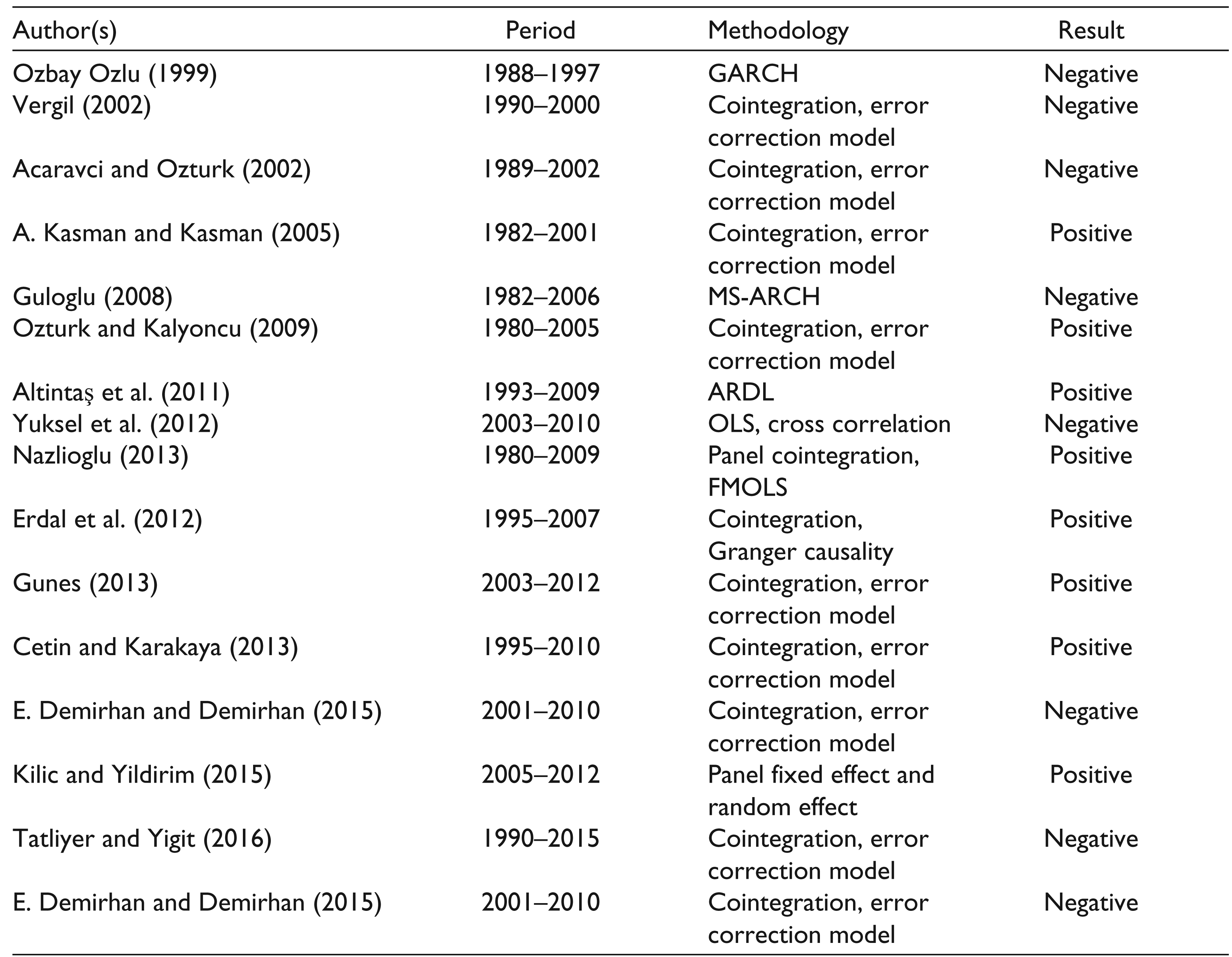
Ozbay Ozlu (1999) is the first paper that analyses the possible impacts of exchange rate uncertainty on exports by using generalized autoregressive conditional heteroscedasticity (GARCH) model for the period 1988–1997. Findings show that exports are adversely influenced by the real exchange rate uncertainty. Vergil (2002) investigates the effect of real exchange rate volatility on the Turkish export to the United States and its primary trading partners in the European Union by launching the data which ranges from the year 1990 to 2001. In the analysis, the standard deviation of the percentage change in the real exchange rate is used as a proxy for exchange rate volatility. According to the cointegration and error-correction models’ results, on the whole, the work concludes that the real exchange rate volatility has a significant negative impact on real exports. Acaravci and Ozturk (2002) perform cointegration and error correction model to observe how the volatility has an impact on Turkey’s export for the period 1989–2002. Their results show the negative evidence of volatility on the export. A. Kasman and Kasman (2005) examine the effect of real exchange rate volatility on Turkey’s exports to its most substantial trading partners for the period 1982–2001. Authors implement cointegration and error correction techniques and their findings imply that exchange rate volatility has a significant positive effect on export volume in the long run. Guloglu (2008) aims to reveal the correlation between exchange rate volatility, exports and exchange rate regimes in Turkey. By applying a nonlinear Markov Switching ARCH technique for the period 1982–2006, the author demonstrates that the periods of high exchange rate volatility usually match with the periods where export performance is low, while the terms of low volatility usually correspond to the periods in which real export growth rates are high. For the time interval of 1980–2005, Ozturk and Kalyoncu (2009) find that the volatility has positive effect on Turkey’s export by conducting residual-based cointegration estimations. Altintaş et al. (2011) searches the effect of real exchange rate volatility on aggregate Turkish exports during the period 1993–2009 by considering the ARDL cointegration technique and error correction model. According to their long-run estimation evidence, the real exchange rate volatility has a positive and statistically significant impact on Turkish exports. Yuksel, Kuzey, and Sevinc (2012) examine the effect of exchange rate volatility on aggregate exports for the period 2003–2011. In their research, they conduct OLS and cross-correlation techniques. According to their highlights, there exists a negative correlation between exports and volatility, but this correlation is not significant at 5 per cent confidence interval. Demez and Ustaoğlu (2012) observe the influence of exchange rate volatility on the Turkey’s export amounts to five top importers including Britain, Russia, Italy, the USA and Germany for the period 1992–2010. They aim at exploring whether both series are influenced by each other in the turning points determined by unit root test with structural breaks. They explore that exports are not influenced by structural turnings in currencies and claim that export is not responsive to the structural breaks and changes in currency rates. Nazlioglu (2013) inspects the outcome of the exchange rate volatility on Turkey’s export from top 20 export industries to primary 20 trading partners during 1980–2009 through panel data techniques. The results indicate that the impulse of the exchange rate volatility on Turkish export shows alteration across industries. According to panel fully modified ordinary least square (FMOLS) results, the volatility has positive impact on Turkish industry-level exports. Erdal et al. (2012) question the impact of the volatility on agricultural export and agricultural import in Turkey by following the period 1995–2007. According to their results, positive long-term relationship appears to be available between volatility and agricultural exports while there happens to be negative response of agricultural imports. Considering the cointegration and vector error correction models, Gunes (2013) analyses the connection between exchange rate, export and import for the period 2003–2012. He concludes that the exchange rate has positive impact on export. Cetin and Karakaya (2013) examine the possible long-run and short-run effect of the volatility on Turkish exports of electrical goods within the period 1995–2010 by performing cointegration and error correction techniques. They eventually imply that the volatility influences the export of electrical goods positively and significantly in the long run. E. Demirhan and Demirhan (2015) study the significance of exchange-rate stability on real export size by following cointegration and the parsimonious error-correction procedures to specify long-run and short-run connection between real export volume and relevant determinants for the period 2001–2010. They indicate that exchange-rate stability has a significant positive impact on real export size in short and long runs. They reach, as well, that the volatility has negative consequence on real export size. Kilic and Yildirim (2015) estimate the potency of exchange rate volatility on Turkish real export size for 22 manufacturing sectors following the data ranging from 2005 to 2012 through panel data analysis. They predict the sectoral real exchange rates and sectoral real exchange rate volatility and state that sectoral real exchange rate volatility yields positive and significant impact on sectoral export size. Applying cointegration, vector error correction and causality tests, Tatliyer and Yigit (2016) research the correlation between exchange rate volatility and foreign trade for the period 1990–2015. They explore that exchange rate volatility results in negative impact on Turkish export in the short run. Table 1 briefly summarizes the relevant seminal articles in terms of research period, methodology and output.
One may observe from Table 1 that the literature evidence has mixed output that arises most likely due to the differences in methodologies of the relevant works. As we present in the third section, this work, to the best our knowledge, is the first one which considers the structural breaks (regime shifts) to inspect the possible time varying sequence of volatility on export in Turkey. Thereby, this work aims at (a) uncovering the break dates, if exists, in the estimated model, (b) revealing the significances of the regressors on regress and within regime switching conditions and (c) unveiling, as well, the consequence of volatility and other dependent variables on dependent variable of export.
A Brief Relevant Literature Review for Turkey
The Model, Data and Methodology
Our model is based on the traditional long-term aggregate export demand with exchange rate volatility. Thusly, we consider the regression equation in logarithmic form as follows.

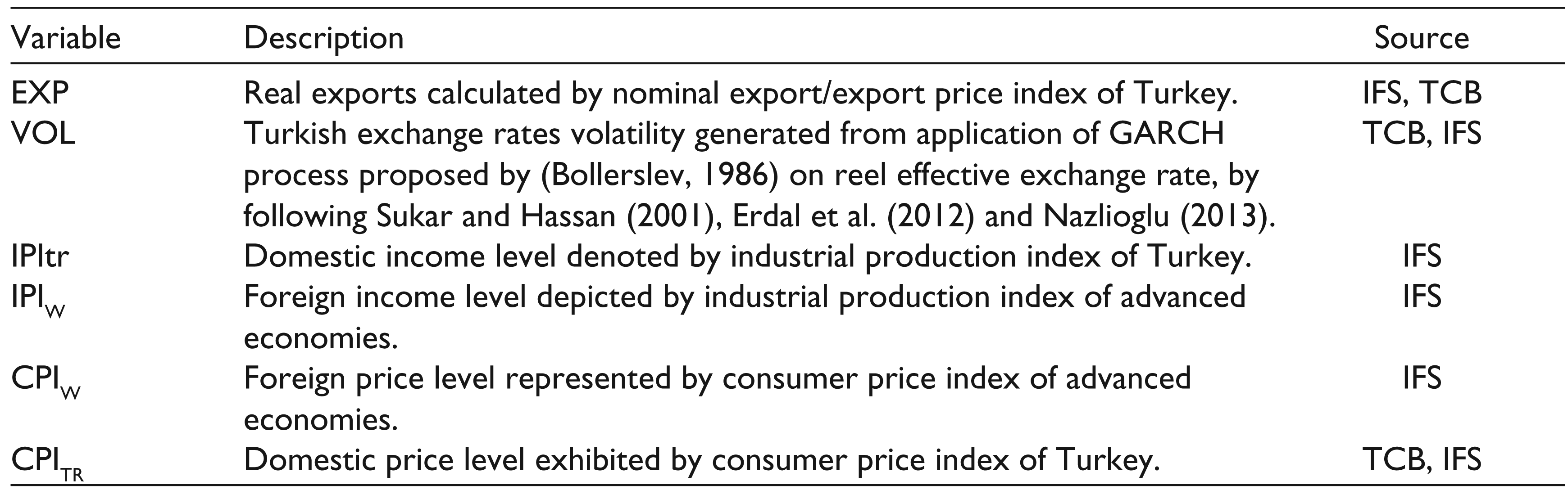
where ln(EXP), ln(VOL), ln(IPI)TR, ln(IPI)W, ln(CPIW /CPITR) and Ɛ represent the logarithmic levels of real export, the volatility in real exchange rate, industrial production index as proxy for Turkish domestic income, industrial production index as proxy for world income, the ratio of world consumer price index to the Turkish price index and random error/innovation term, which is independent and identically distributed, at time t, respectively. Each original time series was seasonally adjusted to remove seasonal effects from the regarding series. Thereby, the seasonal fluctuations have been disappeared in the data. Table 2 lists the series to show their sources and to depict how they are calculated.
According to the relevant theoretical explanations, one might expect positive signed coefficients of foreign income and foreign price level. In view of Turkish export experience from past to present, the exports have been heavily dependent on imported inputs of intermediate goods and/or raw materials. So the coefficient of the domestic income is also expected to have positive sign. Despite a widespread opinion indicating that an increase in exchange rates volatility reduces export, there is no real consensus on the direction or the size of the exchange rate volatility (Sukar & Hassan, 2001) and the effect of exchange rate volatility may change period by period over time. Hence, we will investigate basically the effect of exchange volatility on the exports by estimating the coefficients in Equation (1).
Table 3 depicts the descriptive statistics of ln(EXP), ln(VOL), ln(IPI)TR, ln(IPI)W and ln(CPIW/CPITR), respectively. The maximum and minimum points of exports are 9.751 and 8.085, respectively, for instance. The values of 9.751 and 8.085 might represent a possible peak and trough within the cycles of ln(EXP) series. Then, one might claim that a GARCH model of volatility in real exchange rate might capture better the possible potential significant extreme points of the fluctuations of ln(EXP).
One may observe, as well, that the considerable difference(s) between maximum and minimum values which appear in ln(VOL), ln(IPI)W and ln(CPIW/CPITR). The negative minimum point of ln(CPIW/CPITR) stems from the logarithmic values less than 1. The relatively smaller values of standard deviation occur in the series of ln(IPI)TR and ln(IPI)W, as the greater standard deviations exist in ln(VOL) and ln(EXP). Figure 1 points out the fluctuations in ln(EXP) series.
Data Description, 2003:01–2015:04
Descriptive Statistics, 2003:01–2015:04
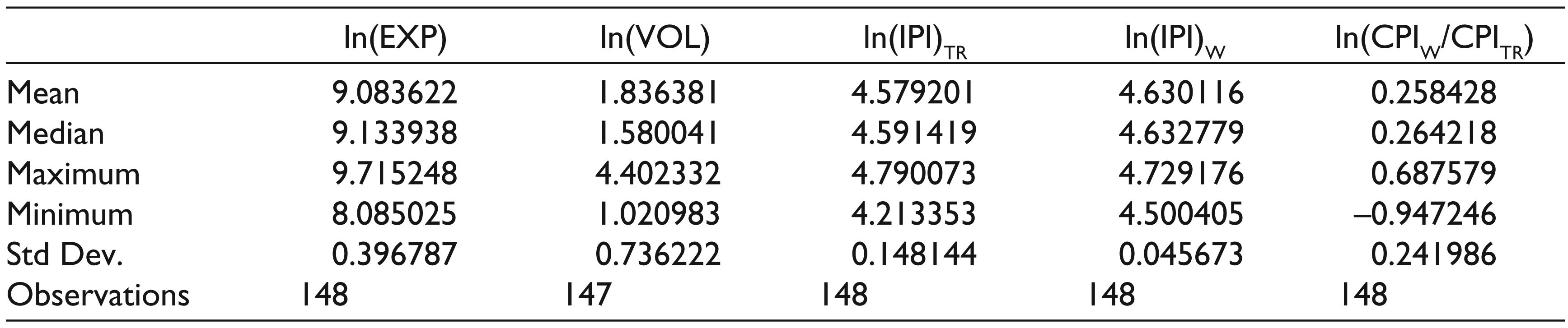
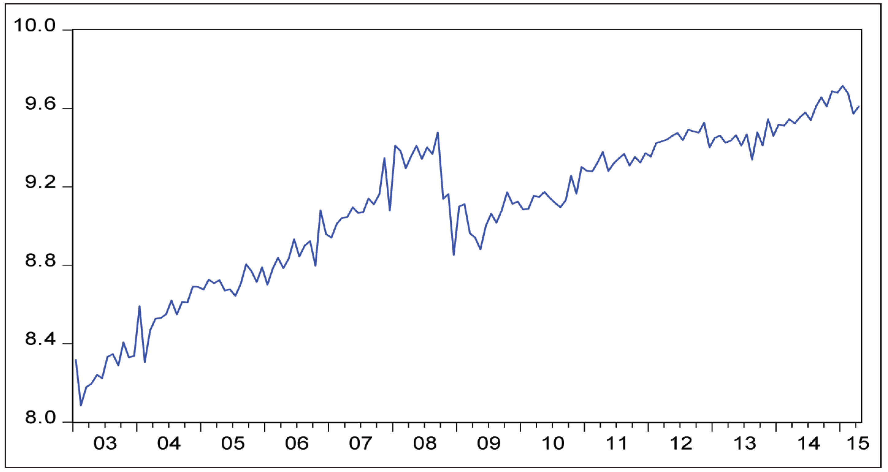
Figure 1 indicates (a) the peak points of 2004:01, 2006:11, 2007:11, 2008:09, 2009:10, 2010:06, 2011:04, 2012:11, and, 2015:01, and, (b) the trough points of 2004:02, 2005:07, 2006:10, 2007:12, 2008:12, 2009:5, 2010:08, 2012:12, 2013:08 and 2015:03, respectively.
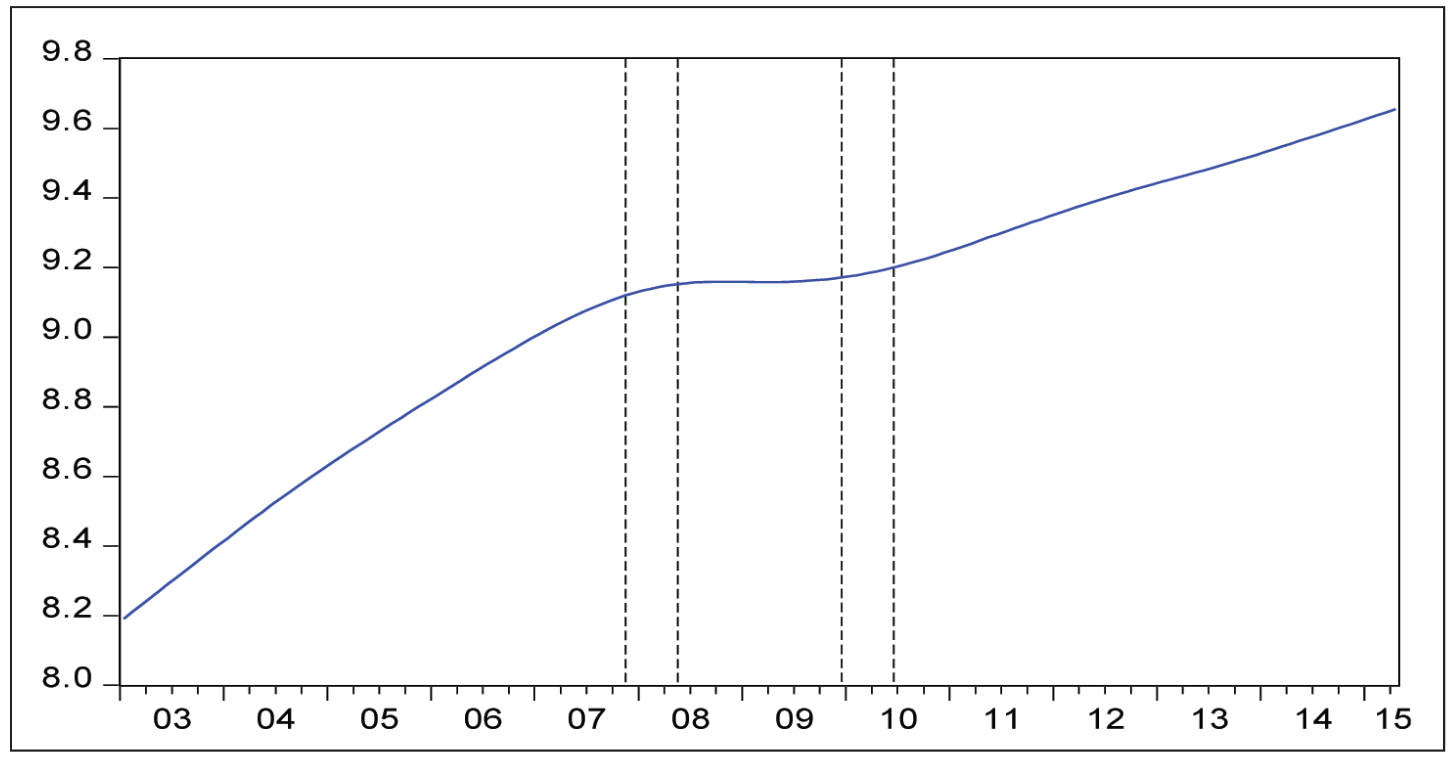
Figure 2 exhibits the smooth estimation of exports through Hodrick–Prescott methodology to obtain the long-term trend component of the exports series in logarithmic form. Then Figure 2 reveals that the relatively greater changes in slope of exports’ curve which appear at 2007:11, 2008:05, 2009:12 and 2010:06, respectively. One may inspect visually that these time points might correspond to regime shifts or breaks of long-run path of exports’ curve. One, on the other hand, needs to follow more reliable inspection to detect the regime shifts of all independent variables as well as dependent variable of exports through iterations with strong convergence by several statistical methodologies.
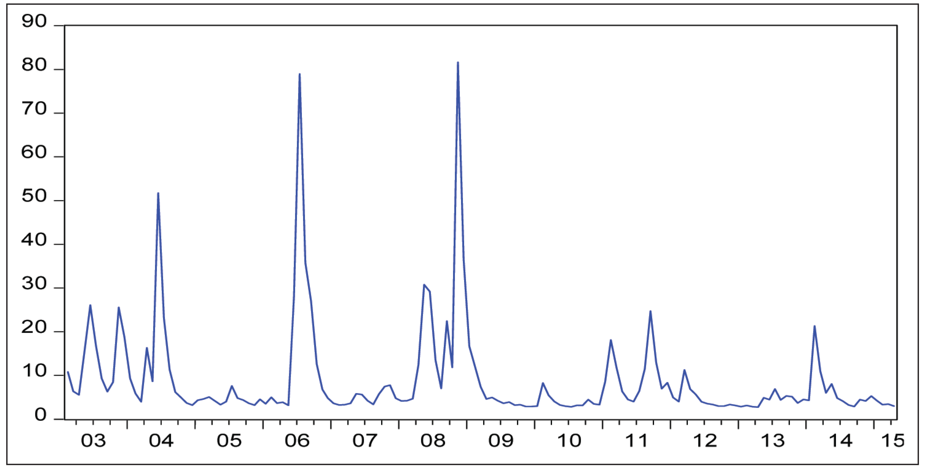
One of the regressors is the volatility as depicted by Equation (1). Figure 3 shows the volatility in real exchange rate which is the conditional variance estimated by GARCH (1, 1) model.

Following Equation (2), the heteroscedastic variance at time t in a GARCH (1,1) model is the function of a constant, squared residuals at time t–1, and the variance at time t–1 as is given in Equation (3).
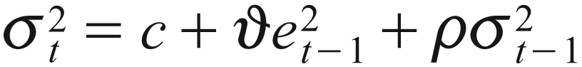
where
Figure 3, then, yields conditional variance graph exhibiting the periods of high volatility in Turkish real exchange rate. Turkish exchange rate volatility spikes up and then drops back relatively more sharply during 2003:06, 2003:11, 2004:06, 2006:07, 2008:06, 2008:11, 2011:02, 2011:09 and 2014:02. The sharpest volatilities appear on July 2006 and November 2008.
The main task of this article is to predict the variance of exports by observing the conditional variance of real exchange rate (volatility).
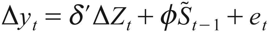
Before the prediction of correlation between two series’ variances, we need to launch preliminary statistical tests to understand whether or not the series has unit root in order to avoid spurious results from the regression estimations. Lee and Strazicich (2003) propose a two-break minimum Lagrange multiplier (LM) unit root test in which the alternative hypothesis unambiguously implies trend stationarity. There are two other unit root tests, considering two structural breaks by Zivot and Andrews (1992) test (hereafter, ZA test) and Lumsdaine and Papell (1997) test (hereafter, LP test). The important issue for ZA and LP is that they assume no break under the unit root null and derive their critical values accordingly. Thus, the alternative hypothesis means that structural breaks are present while the series might have unit root. In this respect, LM test suggested by Lee and Strazicich (2003) allows breaks under the null and alternative and takes into account existence of unit root.
Additionally, the optimal number of break points is endogenously determined. Two-break LM unit root test statistics are derived as follows:
where
In the case of non-stationarity, one might get biased and inconsistent results from the regression equations. Although the variables of interest might be individually nonstationary, [I(d), as d≠0], one or more linear combinations of those variables might be stationary. Hatemi-J (2008) proposes a residual based cointegration test which considers two structural breaks in order to test for linear combination of the variables. Hatemi-J (2008) modifies augmented Dickey-Fuller test, ADF, (proposed by Engle & Granger, 1987), Za and Zt tests (suggested by Phillips, 1987) by extending the tests with two structural shifts based on

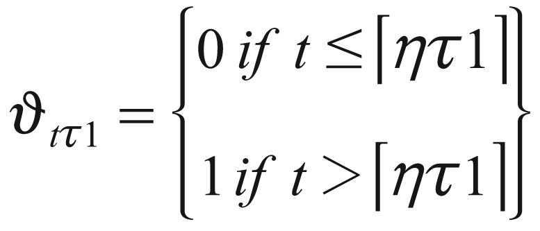
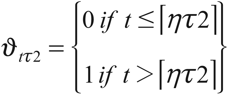
where D1t and D2t are dummy variables for breaks in level while D1txt and D2txt represent regime shifts in the equation. Dummy variables are determined as Dit = 0 if t ≤ [nτi] otherwise 1, and they consider the breaks determined by the underlying data rather than a priori information. Here t, n and the term in bracket denote time index, number of observation and integer part, respectively. Then ADF test statistics calculated through t-test for the slope of estimated error term of ut in Equation (3) in order to test the null hypothesis of no cointegration. The calculations of the Za and Zt tests are based on the first-order serial correlation coefficient
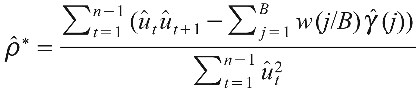
where w(.) meets the standard conditions for spectral estimators, and it is a function yielding Kernel weights. B is the bandwidth number and
The practicable test statistics are minimum values of these tests across all values for τ1 and τ2, with τ1 ϵ T1 = (0.15,0.70) and τ2 ϵ T2 = (0.15 + τ1,0.85). The reason behind selecting the minimum value for the tests is that minimum value provides evidence against the null hypothesis. The test statistics can be formulated as given in Equations (9), (10) and (11).
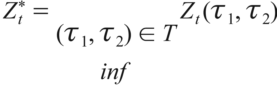
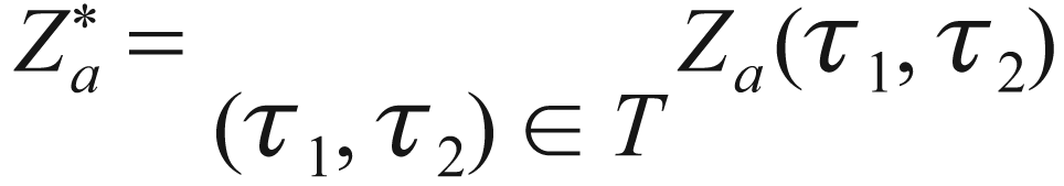
where T = (0.15n, 0.85n), as it trims the data by 15 per cent on each side, this trimming procedure comes from Gregory and Hansen (1996). Following the same justification, Hatemi-J (2008) also let distance between the two regime shifts be at least 15 per cent.
The cointegration states the existence of an equilibrium and long-run relationship between two or more time series, each of which has non-stationary process and long-run coefficients should be determined to understand the magnitude and sign of cointegration. The standard least squares dummy variable estimator is consistent, but suffers from second-order asymptotic bias that causes test statistics diverge asymptotically (Phillips & Hansen, 1990). Phillips and Hansen (1990), Park (1992), Stock and Watson (1993) follow FMOLS, canonical cointegrating regressions and dynamic ordinary least squares (DOLS) estimator, respectively, so as to determine the long-run coefficients. The relevant estimators deal with the problem of second-order asymptotic bias arising from serial correlation and endogeneity. Thus, the errors are allowed to be serially correlated and the regressors are allowed to be endogenous within regarding procedures.
This research follows mainly the analyses of cointegration through regime shifts to estimate basically, if exists, the possible significant influences of the volatility in exchange rate on export volume of Turkey. The research also conducts the cointegration equilibriums through DOLS and FMOLS to confirm/disconfirm the output from cointegration equilibrium with regime shifts. In order for the relevant model to be specified well, the industrial production of Turkey, industrial production of World, the World price level to Turkish price level ratio are, as well, observed as shown in Equation (1). Hatemi-J (2008) launches cointegration tests with two regime shifts depicted by Equations (12–16).
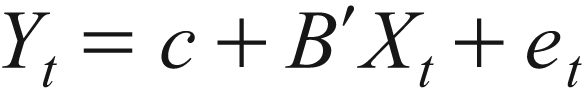
where Yt, c, B', Xt and et denote the vector of a dependent variable, constant, transpose of beta and X matrix of regressors and residual vector at time t, respectively. When residuals are I(0), Yt and X t are considered cointegrated variables. A cointegration estimation assuming that c and B do not vary over time might result in biased output, if the true data involves the regime shift(s) in B and/or c through time. Hatemi-J searches for the possibility of two unknown regimes. Then the dummy variables capture the break date 1 (regime shift 1) and break date 2 (regime shift 2) as depicted in Equations (13 and 14).
Equations (15 and 16) are to estimate (a) the model with regime shifts in constant and (b) the model with regime shifts in regressors and constant simultaneously.


where μt and subscripts (0), (1) and (2) stand for trend, level, regime shift 1 and regime shift 2, respectively.
Empirical Results
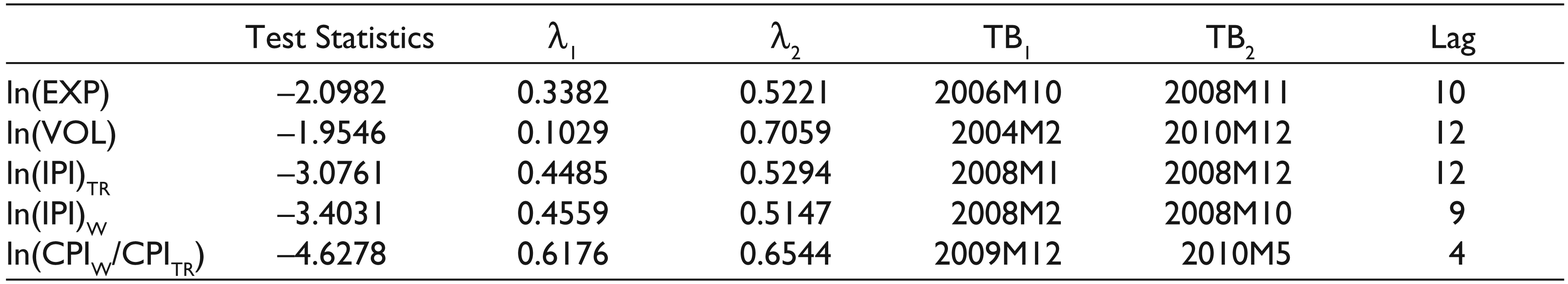
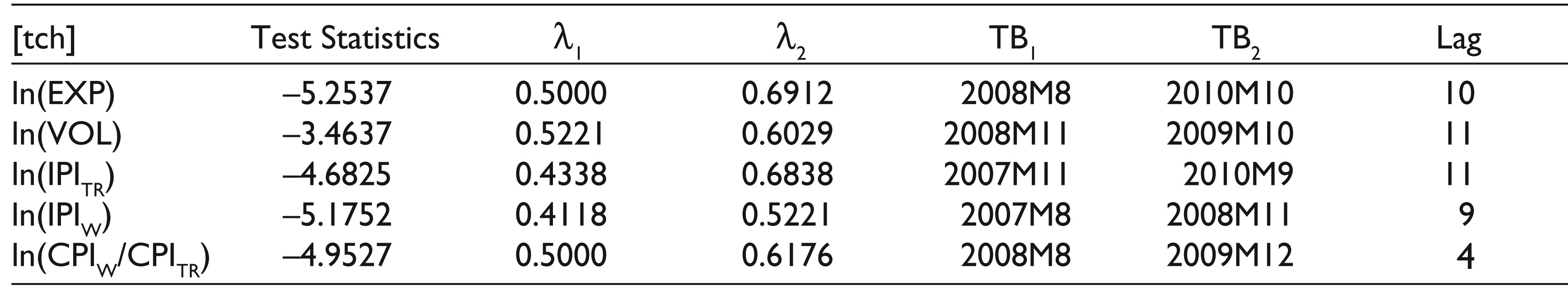
We first apply unit root tests in order to see whether or not the series stationary by following two models. First model (Model A) allows two breaks in level, while the second (Model C) consists of two breaks in level and trend. Results are tabulated in Table 4a and 4b.
The results given in Table 4a output confirms null of unit root, except ln(CPIW/CPITR), and Table 4b yields that the null hypothesis of unit root cannot be rejected for each series under the existence of structural breaks. The series, hence, follow non-stationary process. In the case of non-stationarity, one would get spurious results from the regression equations. It’s quite possible to obtain a linear combination of integrated variables that is stationary, then, such variables are said to be cointegrated, and they have an equilibrium relationship in the long run. Equilibrium relationship means that the variables cannot apart from each other independently (Enders, 2010). The time points of break points are estimated differently for each series as the specific factors affect the mean of relevant time series. This is an important implication for the non-stationary series used in the investigation of long-run relationships. After conducting the unit root tests with structural changes, we applied cointegration tests of Hatemi-J (2008) to investigate the possible existence of long-run relationship among them. The results are exhibited by Table 5.
The Minimum LM Unit Root Test Results for Model A
The Minimum LM Unit Root Test Results for Model C
Hatemi-J’s (2008) Tests for Cointegration with Two Regime Shifts
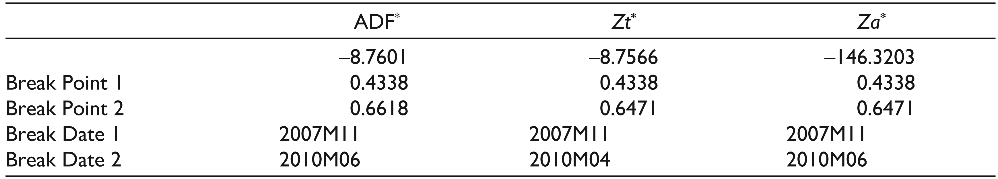
Table 5 reveals that the null hypothesis of no cointegration is rejected by ADF*, Zt* and Za* at 1 per cent significance level, by allowing two regime shifts in cointegrating relationship. The eleventh month of 2007 was determined as the first break point by the all test statistics. Fourth month of 2010 was determined as the second break point by Zt*. The other two tests, however, determined second break in the sixth month of 2010. These break points imply serious deviations on the linear combination of the series. The breaks coincide with the important changes in Turkish economy, especially in terms of exports and real exchange rate. In this way, the detected breaks should be included into the analysis so as to yield more reliable and efficient results.
Having concluded that exports, exchange rate volatility, domestic income, foreign income and the ratio of foreign price to domestic price are cointegrated, we next examine the interaction between these variables using long-run cointegration estimators. The regression equation explained in Equation (1) was expanded with structural breaks determined in cointegration analysis by using dummy variables.
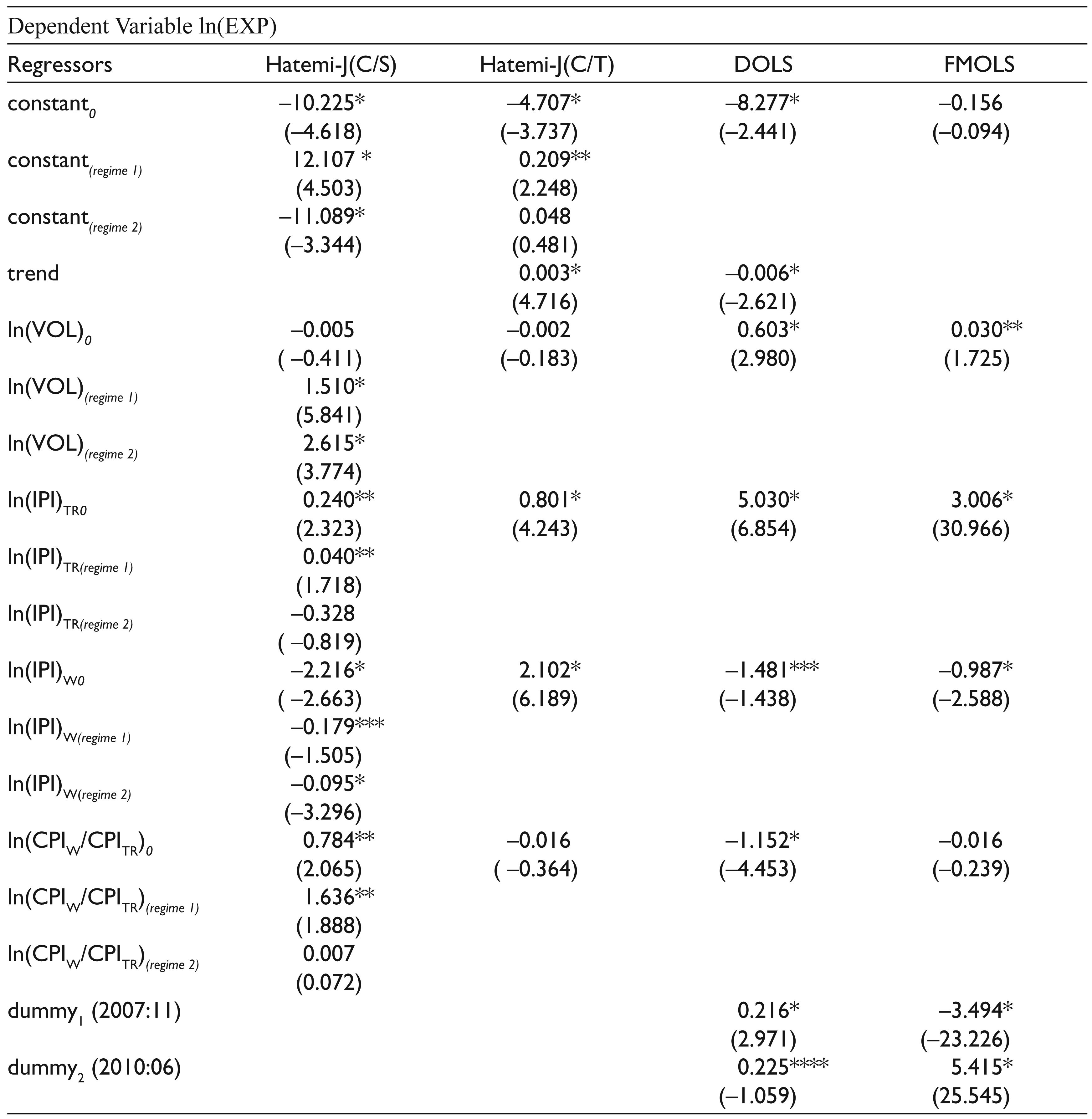
Therefore, we estimated four models given in Table 6a. The first model is the cointegration model with regime shifts in constant and in regressors (second column, Hatemi-J[C/S]). The second model considers estimating the cointegration model with trend and all regressors and the regime shifts in constant (third column, Hatemi-J[C/T]). The third and fourth models (fourth and fifth columns) follow the cointegration analyses from FMOLS and DOLS, respectively, with dummy variables of 2007:11 and 2010:06. We need to mark here that the break points of 2007:11 and 2010:06 are entered into FMOLS and DOLS exogenously as these break points are detected endogenously by first and second models.
The second column of Table 6a yields Hatemi-J(C/S) estimation output and indicates that the constant at time t (constant 0 ), the constant at first regime (constant (regime 1) ), and constant at second regime (constant (regime 2) ) are found statistically significant. The volatility (ln(VOL)) appears not to be significant at the level (ln(VOL) 0 ) but seems to be significant at regime 1 (ln(VOL) (regime 1) ) and at regime 2 (ln(VOL) (regime 2) ).
A careful interpretation is required at this stage. The estimated coefficient of volatility is not significant on exports (ln(EXP)) until the first break time (November 2007). The coefficient becomes significant at first break time (first regime) and continuous to be significant till the end of data period. Therefore, the volatility takes the significant positive value of 4.12 (= –0.005 + 1.510 + 2.615) on exports from 2007:11 to the end of 2015:4 which is the end of the sample period. The domestic income (ln(IPI)TR) is significant at time t, with the estimated value of 0.240 and at first regime with the value of 0.040. This result depicts that domestic income can influence the export positively for the period 2003:01–2010:06 with the coefficient of 0.28 (= 0.240 + 0.040). One per cent increase in domestic income leads to 0.28 per cent increase in exports. As the world income (ln(IPI)W) increases by 1 per cent, the Turkish export volume diminishes by 2.49 per cent (= –2.216 – 0.179 – 0.095) for the period 2003:01–2015:04.
The DOLS results reveal that volatility and domestic income have significant positive power on exports, whereas the world income and price ratio have negatively significant sequences on export. The FMOLS output yield that increase in volatility and domestic income cause export to increase significantly, whereas the increase in world income leads exports to decline significantly. The price ratio is not found significant by FMOLS estimations.
Table 6a, second column explores, as well, that, when the ratio of world price level to the Turkish price level (ln(CPIW/CPITR)) goes up by 1 per cent, the exports of Turkey boosts by 2.42 per cent for the time interval of 2003:01–2010:06. The price ratio at second regime, from 2010:06 to 2015:04, is found insignificant.
One may depict eventually, throughout regime shifts analyses, that volatility, domestic income and price ratio have significant positive impacts on exports, while the world income has significantly negative effect on the export volume of Turkey. The third column of Table 6a yields Hatemi-J(C/T) estimations in which the possible regime shifts are considered only in constant term. The estimation explores that (a) constant terms at time t and at the first regime appears to be significant, (b) the trend term seems to be significant and positive, (c) the volatility emerges to be insignificant and (d) the domestic income and world income influence export positively significant. The Hatemi-J(C/T) estimations confirm the positive effect of domestic income on export shown in Hatemi-J(C/S) model but disconfirm the negative impacts of world income given in Hatemi-J(C/S) estimations.
The Cointegration Estimates with Regime Shifts (Hatemi-J), Dynamic (DOLS) and Fully Modified (FMOLS)
Goodness of Fit
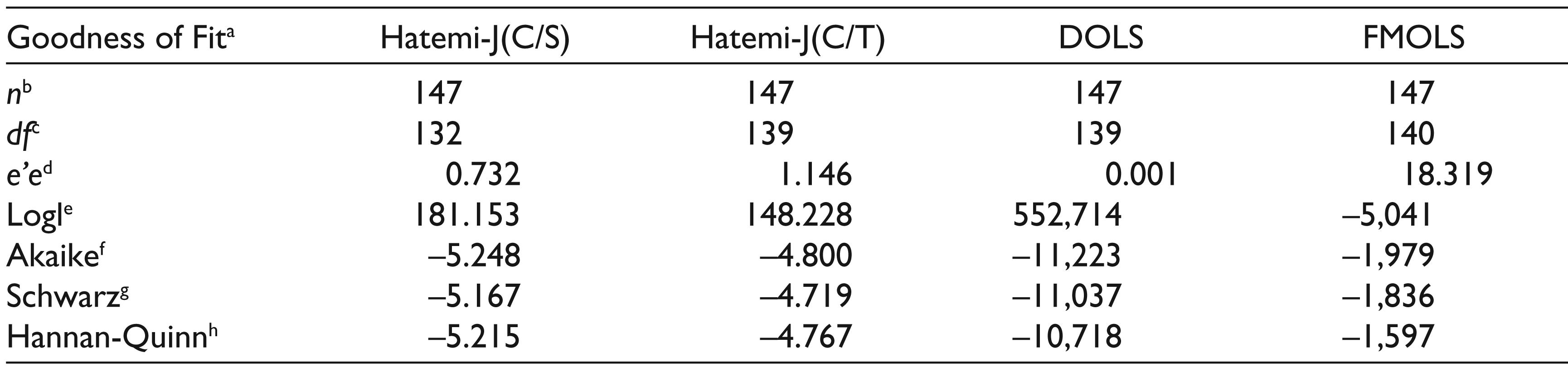
b n shows the number of observations.
c df indicates the degrees of freedom.
d e’e denotes the sum of squared residuals.
e logl explores the log likelihood statistic.
f Akaike represents the Akaike information criteria statistic.
g Schwarz yields the Schwarz information criteria statistic.
h Hannan-Quinn exhibits the Hannan-Quinn information criteria statistic.
The estimations from Hatemi-J(C/S), DOLS and FMOLS support each other regarding the significances and signs of volatility, domestic income and foreign income for Turkish economy. They differ from each other concerning either significance and/or the sign of the price ratio.
Table 6b gives the goodness of fit statistics of four models. The statistics exhibit that the first and second best models among four models are DOLS and Hatemi-J(C/S), respectively, considering the statistics of sum of squared residuals, log likelihood, Akaike information criteria, Schwartz information criteria and Hannan-Quinn information criteria. The higher the log likelihood, the better the data fits model, and the lower the Akaike, Schwarz and Hannan-Quinn statistics, the more the model will be ‘true’ upon the estimations of log likelihood. The output from the all estimators reveals that exchange rate volatility has positive effect on export and is statistically significant. One may expect to find positive coefficients for domestic income, foreign income and price ratio based on the basic classical theory of demand for export. Our results indicate, however, that, as domestic income and price ratio yield positive significant effects, the foreign income explores the negative influence on export. The latter output indicates that the Turkish exported commodities might be considered inferior on average.
The empirical results of this article might exhibit some managerial implications: Due to evidence of inferiority of Turkish exported goods and services, one may suggest that Turkish sectors’ exports shift from high level income countries (e.g., USA, EU, UK, Canada, Germany, Japan) to relatively lower income countries (i.e., MENA countries: Algeria, Armenia, Azerbaijan, Bahrain, Djibouti, Egypt, Iran, and Islamic Republic of Iraq, Israel, Jordan, Kuwait, Lebanon, Libya, Mauritania, Morocco, Oman, Qatar Saudi Arabia, State of Palestine, Sudan, Syrian Arab Republic, Tunisia, United Arab Emirates, Yemen and Western Sahara). This shift might help Turkey increase her exports level quantitatively. The Turkish exporters might be considered risk lovers rather than risk-averse since they respond more positively to the higher volatilities of exchange rates. Then, Turkey’s exports to the low income countries could be increased further in the high volatility periods.
The Theoretical and Empirical Facts Underpinning the Estimation Output
Development policies of Turkey have changed from import substitution industrialization to export-oriented industrialization strategy and liberal policies have been put into practice since 1980. Exchange rates have been closely followed by the administrators to compete with rival economies since then. In this respect, the strategies to fight low-cost rivals have become more important issues. Therefore, the major currencies preferred by economic agencies in the world for international trade appreciated the currencies against the Turkish lira (TL). So, eventually, the Turkish economy has experienced several devaluations. Then, Turkey has shifted from the pegged exchange rate regime to the flexible exchange rate system in 2001. Since then, unexpected fluctuations in exchange rate, more precisely, the volatility has had a great importance in trade flows for Turkey. Empirical results show that the volatility positively affects the export in Turkey. This result might be confirmed by Figures 4 and 5.
This article mainly reveals the long-run parameter estimations of independent variables to understand the behaviour of Turkish exports throughout estimated break points/regime shifts. The estimated positive coefficients of domestic income and the ratio of foreign price level to domestic price level seem to be theoretically correct and are confirmed mainly by the literature evidence. The estimated signs of volatility and foreign income, on the other hand, continue to be a matter of debate. The negative consequence of foreign income on Turkish export implies that Turkish export goods might be inferior. The positive effect of volatility on Turkish export volume might indicate that the firms are risk lower. They are willing to take on additional risk for an investment project to catch the new greater revenue/profit opportunities. We present here some theoretical and empirical evidence underpinning this work’s estimation output regarding break points, the positive impact of volatility on export and the inferiority of export goods.
Break Points
This article takes into account of structural breaks and/or regime shifts for Turkish export model in which the determinants of exports are explored through potential possible significant regime shifts occurred in Turkish economy within the estimation period. Therefore, this article contributes the literature by considering structural breaks that may stem from policy changes or various internal/external shocks, which might be connected with the relevant variable(s), may lead to inconsistent estimation and invalid inference if they are ignored (Baltagi et al., 2016).
The article first aims at revealing the output of cointegration tests throughout the estimations of break points or structural breaks of export, volatility, domestic income, foreign income and the ratio of foreign price level to domestic price level series. The November 2007 is determined as the first break point by the all three test statistics. April 2010 is observed as the second break point by one of three test statistic, as the other two tests detect the May 2010 as the second break. We introduce some basic facts regarding the time points of 2007:11 and 2010:6 here.
In 2007, especially in third quarter of 2007, the economy was under the influence of developments such as the mortgage problems abroad, climbing oil prices, the presidential election process, general elections, referendum and terrorist incidents in the country and the cross-border operation of Iraq (CNNTURK, 2007). According to the indicative exchange rates of the Central Bank, the effective selling price of the US dollar and Euro were 1.4145 TL and 1.8632 TL, respectively, at the end of 2006, and the effective selling price of the US dollar and Euro became 1.1753 TL and 1.7255 TL, respectively, on 15 November 2007 (CNNTURK, 2007; Döviz-arşiv, 2007a; 2007b). In the foreign exchange market, the dollar/TL rate, which was 1.45 at the beginning of 2010, rose to 1.60 during the mid of 2010 due to the impact of the global risk followed by the debt problems of Euro Zone countries. The US dollar/TL exchange rate, which fell below 1.40 in November, rose to 1.55 at the end of the year, as the CBRT loosened its monetary policy (TEB, 2010).
The Positive Influence of Volatility on Exports
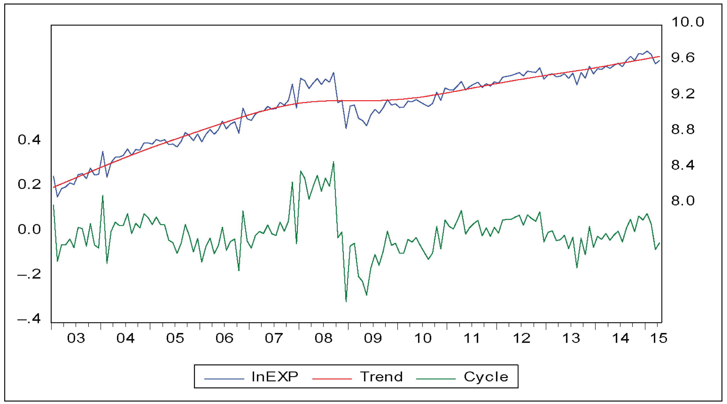
The underlined output of this work is the positive sign of volatility on export. Figure 4 exhibits the trend and cycles of natural logarithm of Turkish exports volume (lnEXP).
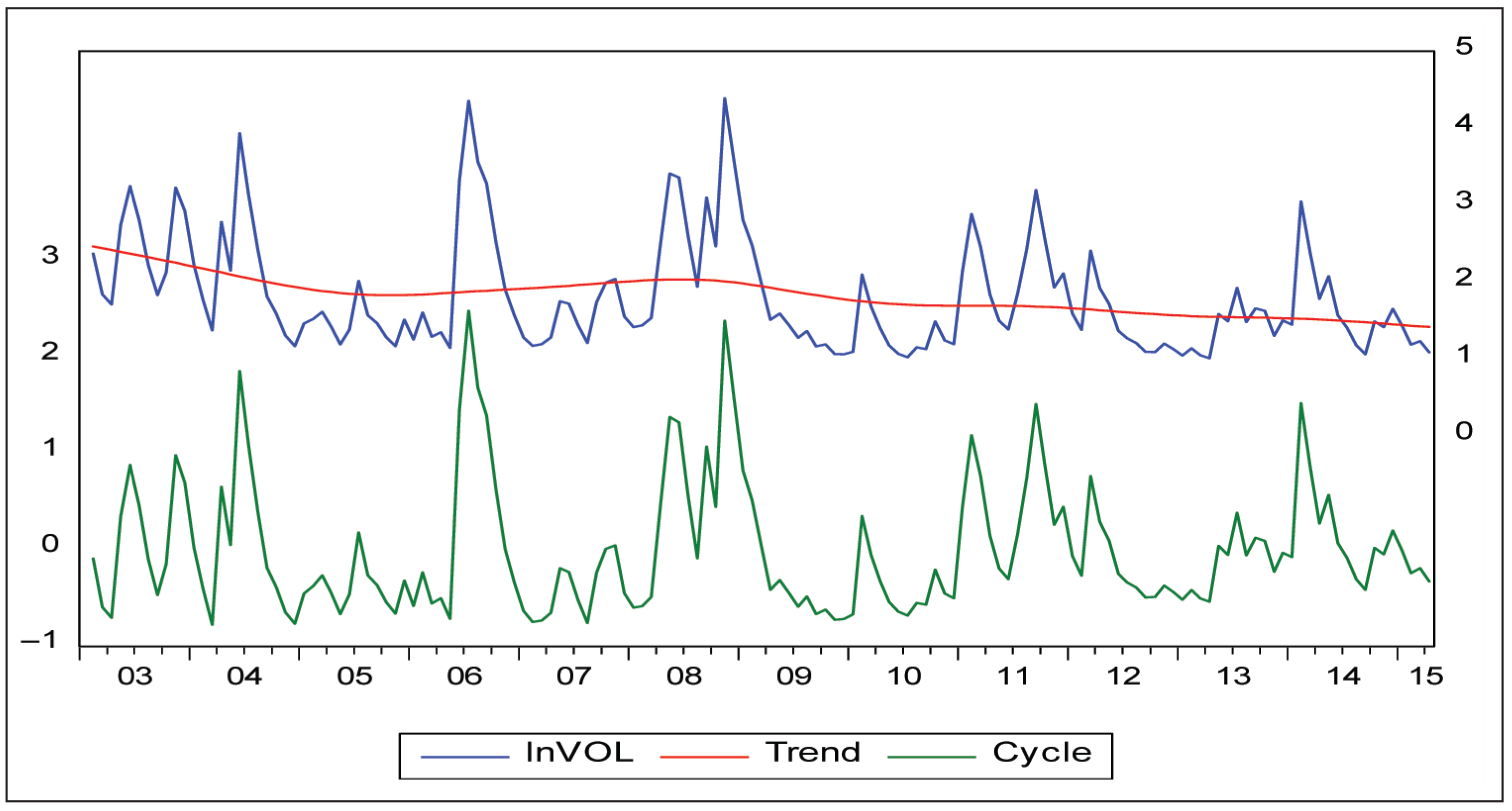
Figure 5 denotes the trend and cycles of natural logarithm of exchange rate volatility in Turkish economy (lnVOL). The trend and cycles given in Figure 4 indicate that the lnVOL cycles of period 2003:01–2008:12 seem to be larger than those of period 2009:01–2015:04. The lnEXP, first, increases at increasing rate (2003:01–2008:12), later, increases at decreasing rate till the end of sample period (2015:04). The Turkish exporters appear to respond more to higher volatility.
Figure 5 depicts that, although there exists ups and downs in the trend of volatility in cubic form depicted by red coloured, the volatility has a decreasing tendency after 2008:12. Figure 4 denotes a relatively diminishing tendency in the growth path of exports of Turkish economy after 2008:12.
The higher the volatility and the higher the frequency of volatility, the more frequent the depreciation and appreciation will be experienced. The depreciation of TL enables companies in Turkey to increase their exports. The public opinion and, so government representatives, strongly argue that the depreciation of TL helps to improve the competitiveness of Turkey and they try to induce the Central Bank to do so in order to increase exports and foreign earnings. However, exports heavily depend on imported inputs such as intermediate goods, raw materials and energy in Turkey. As a result, the depreciation of TL leads to increase in cost of production, as well.
One may eventually notice throughout depreciations and appreciations that the Turkish economy has experienced enormous increases in Turkish exports since 2001 and that liberal policies and floating exchange rate system have appeared to help Turkish economy increase her macroeconomic economic performance.
The positive impact of volatility on exports is confirmed by A. Kasman and Kasman (2005), Ozturk and Kalyoncu (2009), Altintaş et al. (2011), Nazlioglu (2012), Erdal et al., (2012), Cetin and Karakaya (2013) and Kilic and Yildirim (2015). One might argue that although volatility in the exchange comprises some risk it might provide the businesses with opportunities to reach greater profits (Grauwe, 1992; 1998; Van, 2011). The volatility, due to depreciation, causes an increase in volume of exports.
The higher the rate of depreciation is, the higher the demand for exported goods will be. Another outstanding reason, then, of positive effect of volatility on export volume might be the depreciation rates in Turkey. The depreciation will expand, hence, the Turkish export volume. Berument, Coskun, and Sahin (2007), considering day of the week effect of the daily depreciation of the TL against the US dollar and its volatility for the period 12 March 2001–22 November 2005, search the association between volatility in exchange rate and depreciation in Turkey and reach the evidence of positive correlation between exchange rate volatility and the daily depreciation rate. They conclude that a decline in depreciation of TL leads to more volatility in exchange rate than an increase in depreciation. Karagöz (2016), investigating the Turkish export performance for the period 1980–2010, explores that Turkish exports increases as domestic currency remains depreciated. He depicts, as well, that the economic crisis in 2001, when the TL depreciated rapidly, caused Turkish exports to increase due to motivation of new market searches. The significant devaluation might also result in greater level of export. Qian and Varangis (1994) reach positive consequence of volatility on Sweden exports due to prominent devaluation of Swedish krona (Van, 2011).
The Inferiority of Export Goods
One may expect in general that an increase in foreign country’s purchasing power of parity will bring about an increase in quantity demanded for export goods produced/exported by home country. The expectation of positive sign of foreign income might arise from the fact that, according to basic trade models, as host countries income goes up, their demand for export goods, exported/produced by developed home countries, that is, by the USA and UK, will boost. The microeconomic foundations of international trade in observing the link between income and demand, however, explores that the sign of income within demand function depends on the type of commodity or service. The commodities can be classified into three groups in terms of their income elasticities (Ɛiq): (a) the inferior goods (Ɛiq < 0), (b) weak superior goods (0 < Ɛiq < 1) and (c) the strong superior (luxury) goods (Ɛiq > 1).
The world exports market consists of naturally the commodities and services produced by domestic (home) countries through employment of different level of technologies, several varying qualities of raw materials and/or inputs. Our empirical evidence exhibits the negative sign of foreign income on Turkish export and hence the possibility of inferiority of Turkish exports. The inferiority indicates that as foreign income increases the demand for Turkish export volume diminishes. Günçavdı and Kayam (2017), for instance, point out the possibility of inferiority of Turkish export by the fact that Turkish export has shifted considerably to MENA countries where per capita GDP appears to be relatively low. The per capita GDPs of, for example, Lebanon, Iran, Jordan, Libya, Iraq, Algeria, Tunisia, Egypt are 8.052, 5.376, 4.936, 4.642, 4.63, 4.206, 3.872 and 3.615 USD, respectively (ISTIZADA, 2017). Turkey mainly exports to the EU (44.5%), Iraq, the USA, Switzerland, United Arab Emirates and Iran (EU Commission, 2017).
EU Commission (2017) reports that the Turkish exports of manufactured goods has a considerable share of 84.1% in EU markets. Some services or manufactured commodities might have some inferiority characteristics. Or some determinants might have an inferior role for manufacturing exporters as depicted in Mau (2017). Mau (2017) reveals that the global fixed costs are significantly relevant for services trade and that, according to some firm-level studies, global fixed costs might play an inferior role for manufacturing exporters. The Turkish manufacture sector covers the food products, beverages, tobacco products, textiles, wearing apparel, leather and related products, wood and products of wood and cork (except furniture), paper and paper products, coke and refined petroleum products, chemicals and chemical products, rubber and plastic products, fabricated metal products, electrical equipment, machinery and equipment n.e.c., motor vehicles, trailers and semi-trailers, furniture and other products. Then the income elasticity may vary, as well, according to type of manufacturing. Berument, Dincer, and Mustafaoglu (2014), for instance, observe the individual income elasticities of demand for Turkish products of different sectors and reach some evidence of negative income elasticities of demand for Turkish textile products (Germany) and chemical products (the Netherlands and Greece).
Conclusion
There has been an ongoing debate on the effect of exchange rate volatility on export within the relevant literature. The literature evidence yields, however, the mixed output that might arise, most likely, due to the differences in estimation methodologies or different sample time series data or panel data employed. This article, to the best our knowledge, is the first one which takes into account of the regime shifts to detect the potential time varying consequences of exchange rate volatility on Turkish exports. Therefore, this article, aims at (a) exhibiting the structural breaks (regime shifts), if exists, in the estimated model, (b) exploring the impact of the potential determinants of export following the regime switching models and (c) yielding the magnitude(s) and sign(s) of influences of exchange rate volatility, domestic income, foreign income and the ratio of foreign price to domestic price on exports volume.
Thusly, the motivation of this article lies in two points. First, the article considers mainly the effect of exchange rate volatility on Turkish exports by observing the possibility of structural breaks and/or regime shifts. Second, the article follows both regime switching model (C/S) and regime switching model (C/T) where (C/S) represents the model in which regime changes are observed in constant and in all regressors and where (C/T) denotes the model in which the regime shifts are estimated in constant along with trend of the Turkish exports equation.
The regime switching model (C/S) exhibits the evidence that there exist positive impacts of volatility, domestic income and price ratio (W/Tr) and negative influence of World income on Turkish exports. The DOLS estimations confirm the (C/S) model output except the sign of price ratio.
Thereby, in this article, we analyse mainly the impact of exchange rate volatility on exports in Turkey by launching monthly data spanning from 2003M1 to 2015M4 and constitute a model based on the basic classical model of demand for exports. All series are seasonally adjusted and recalculated in logarithmic forms.
In the analysis, we first implement unit root tests with structural breaks and cointegration test with break points, and later we conduct the long-run coefficient estimations through (a) predictions of regime shifts in constant and in regressors by Hatemi (C/S) methodology, (b) estimations of trend and regime shifts in constant by Hatemi (C/T) model, (c) dynamic OLS with lead(s) and lag(s) by OLS methodology and (d) estimations from fully modified OLS (FMOLS) technique.
The outputs of Hatemi-J(C/S), DOLS and FMOLS confirm each other regarding the significances and signs of volatility, domestic income and foreign income for Turkish economy. They differ from each other concerning either significance and/or the sign of the price ratio. Hence, one may conclude that throughout the estimations of this research volatility in real exchange rate affects the Turkish export positively. This output might arise from the behaviour of Turkish firms which might be willing to catch with the opportunities of considerable changes in depreciation rates in TL. One, hence, can consider Turkish exporter companies ‘risk lowers’ which look for higher profitability within current or new markets. The other prominent result of this article is that the foreign income elasticity of demand for Turkish exported commodities/services is negative. This later output might stem from the inferior characteristics of Turkish export. The inferiority might stand for the cheaper products, that is, cheaper cars or cheaper textile products exported by Turkey to the world exports markets. Therefore, this article might suggest that the Turkish sectors’ exports shift from high level income countries to relatively lower income countries.
This article may further suggest new future potential original researches to confirm or disconfirm the output of this work. One, then, may launch a new data set for a developed country or for an emerging country to inspect the response of exports behaviour to the volatility in exchange rate and other potential regressors by employing the methodologies of wavelet coherency analyses in which time and frequency domain predictions are observed simultaneously. One might consider, as well, new possible independent variables such as consumer confidence index and/or producer confidence index and/or political, economic and financial risk indexes in domestic and foreign markets to depict the path of exports level in detail of a country in the world exports market.
Footnotes
Declaration of Conflicting Interests
The authors declared no potential conflicts of interest with respect to the research, authorship and/or publication of this article.
Funding
The authors received no financial support for the research, authorship and/or publication of this article.