COVID-19 and Dependence Between Oil and Renewable Energy Stocks: C-Vine Copula Approach

Abstract

This article analyses the dependence structure between traditional energy prices traditional oil indices and renewable energy stock indices employing Canonical Vine (C-Vine) copula based GARCH approach. The analysis is conducted before and during-COVID-pandemic period. Renewable energy stock is represented by SPGCE and CLEANTECH index, whereas traditional energy is represented by WTI crude oil and OVX. The empirical analysis indicated increasing asymmetric dependence between WTI crude and renewable energy indices during COVID-19. However, WTI crude oil is not found to be the primary determinant for influencing renewable energy stocks. In fact, we find a strong association between SPGCE and CLEANTECH and degree of dependence escalated during COVID-19 period. Besides this, the dependence structure between WTI crude and CLEANTECH changes from the upper tail dependence to lower tail dependence signifying the consequences of low economic activities on the technology sector. Furthermore, the dependence between OVX and SPGCE conditional on WTI reveal the scope of diversification as dependence parameters are insignificant. These findings are robust considering alternative GARCH specifications and alternative oil future benchmark and renewable energy stock index. The results provide useful implications for the energy policymakers and investors.

Keywords

Covid Dependency WTI Crude Energy Stock Vine-copula

Introduction

‘These are the unfortunate repercussions of a global market that’s exposed to the volatility of the oil markets and suffers when unforeseeable events like coronavirus arise at the worst time. We are now seeing the downsides of the choices we’ve made about the kind of energy economy that we have.’¹

Dr Charlie Donovan, CCFI, Imperial College Business School, London

Over the years, investment in renewable energy has gained momentum globally with the focus to increase its share in the overall energy mix portfolio. Renewable energy is often described as clean energy, which is obtained from the natural resource such as wind, solar, biomass and hydropower.

The Paris Agreement was signed by 194 countries and enforced on 04 November 2016.² Countries have also given their consent to Nationally Determined Contributions plan including using renewable energy to reduce the global emission.77 countries have announced to attain net zero carbon emission by 2050 by prioritizing energy efficiency.³ The growing trend of investing in renewable energy reflects both the cost-effectiveness and public interest in renewable resource. For instance, global use of renewable energy rise by 1.5%, whereas production of electricity through renewable grow by 3% in Q1 of 2020 compared with the same period of 2019. This is partly attributed to the new solar and wind installations accomplished in the last few years and renewable having low marginal operating costs.

Before the onset of COVID-19, the transition to clean energy was being undertaken in many countries. The alternate source of energy became remarkably affordable due to rapid technological progress and solid policy framework to promote environmentally friendly sources of energy. Along with that, climate change and excessive CO₂ emission lead the worldwide interest to shift to clean energy sources. The renewable energy sources like solar and wind have become substantially cheaper in the recent years, and it was being anticipated that soon renewable energy would replace fossil fuels (Hosseini & Wahid, 2016).

Among fossil fuels, oil has the greatest potential to affect the performance of renewable energy and investment, due to high substitution effect (Bondia et al., 2016; Ferrer et al., 2018). On the one hand, fall in oil prices would lead less use of alternate energy as production cost of clean energy is already very high, which would hinder the transformation of high-carbon emitting industries to low-carbon industries. On the other hand, rise in oil prices would provide high incentives to the companies to shift clean energy and thus increases profitability. The firms using oil as input in their production would demand less for oil, which should speed up the transition to renewable energy sources. In addition, movement of oil prices are often impacted by geopolitical tensions as oil prices are largely regulated by OPEC nations. Intuitively, risks arising from geopolitically tensions are likely to transmit to the clean energy market which in turn may impact the investment level of clean energy.

In the last decades, oil prices encountered several extreme upward or downward movements. For instance, crude oil observed the highest downfall in the spot price from USD 144 per barrel to USD 30 per barrel as a consequence of Global Financial Crisis 2008 and brought down the crude oil production and consumption by 1.2% and 1.5%, respectively (IEA). Crude oil prices experienced extreme downward movement with the outbreak of Novel Corona Virus which resulted in the significant drop in the prices of WTI crude oil futures in April 2020 reaching to its minimum price at −$36.98 per barrel (Figure 1). Although it picked afterwards, but the low-price trend continued.

Figure 1.

Movement of WTI Crude Futures (2008–2020).

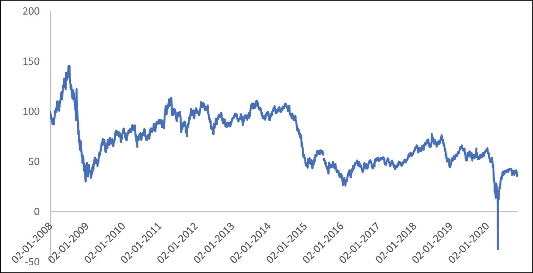
The oil prices volatility typically increases a sense of economic uncertainty. The investors and policy makers may contemplate the role of lower volatility assets (for instance, renewable energy) for achieving stability. The renewable energy may themselves be subjected to other forms of volatility but it has the potential to disconnect the economies from global oil market volatility due to its ability to replace the crude oil in the long run. Hence, renewable energy may offer the hedging against the oil price volatility.

The relationship between oil and renewable is suspected to alter after the outbreak of COVID-19 at least for the following reasons. The novel coronavirus led to the lockdown in the countries. The production was halted. It disrupted supply chains, delayed procurement and so on. Ultimately, it resulted in huge slump in the energy demand. Following the decline in the oil demand, oil prices crashed by 85% between 22 January and 21 April 2020; oil future went negative. Many big oil companies are now expecting the shock of the pandemic to linger on for a longer period, hence writing off their book value or filing for bankruptcy (Khanna, 2020).

The lockdown imposed by the countries has also ramifications for the clean energy sector. The COVID-19 has struck the manufacturing facilities, supply chain of renewable energy companies that slowdown the transition to the renewables. The renewable energy investments and incentive plans were put on a brake by countries to fight against the pandemic⁴. For instance, American-based Morgan Stanley company intended to cut down the installation of the US solar photovoltaics in the second, third and fourth quarter of 2020 by 48%, 28% and 17%, respectively⁵. Renewable energy companies reduced borrowing and production to exercise more financial discipline during COVID-19.

The investment risk in the alternate energy market is generally higher than traditional energy industries. During hard periods, this created a friction between renewable energy and traditional oil companies. Hence, it is realistic to assume that the dynamics between traditional and clean energy are complex but transient, that is, passes through various market circumstances. Therefore, understanding the interplay between oil prices and clean energy sector stock price during the COVID-19 crisis is of interest for investors and policy makers to evaluate the risk exposure and renewable energy policy to reduce the risk of investment in alternate energy sources.

The article contributes to the existing literature in the following ways:

First and foremost, massive literature has been dedicated to explore the effect of oil prices on renewable energy performance previously. Yet, there was no census on the linkage between oil and renewable energy prices. Some studies support that there is weak or no impact of oil prices on renewable energy (Khan et al., 2014; Kyritsis & Serletis, 2019; Omri & Nguyen, 2014; Payne, 2012; Sadorsky, 2009), while other studies support the idea of a strong relationship between them (Dutta, 2017; Ferrer et al., 2018; Reboredo, 2015). In addition, there are studies that reported the relationship between them being not stable, that is, sometimes exist and sometimes recede (Hammoudeh et al., 2021; Maghyereh et al., 2019; Xia et al., 2019).

The possible reason for these contradicting findings could be that there exists structural break in the oil prices, which necessitate the consideration of extreme market conditions. The inspection of extreme shocks becomes necessary as they have valuable information and ignoring them could lead to biased inferences (Choi, 2014). Rational investment decisions take into account the estimation of left and right tails of the distribution. In this article, we applied the copula approach that offers great flexibility in modelling the dependence by considering average as well as tail dependence of the return distributions. This approach is more robust than the one based on parametric bivariate distribution functions since it permits the independent modelling of the marginal behaviour of oil and renewable energy indices. In addition, copula provides the information on the joint extreme co-movements which is highly useful for making portfolio allocation decisions and risk management policies.

In this study, we examine the conditional dependence between oil indices which are represented by WTI Crude Future and Oil Volatility Index (OVX) and two renewable energy indices: S&P Global Clean Energy Index and CLEANTECH Index.

Our study is close to Mejdoub and Ghorbel (2018) who also emphasized the tail dependence and examine dependence structure between renewable energy indices and WTI crude oil. But our article is different from Mejdoub and Ghorbel (2018) in the following aspects. First, we incorporate the Oil Volatility Index (VIX) in the multivariate data setting. The huge swings in the oil price have substantial impact on the financial markets by creating continuous risks and uncertainties. Celik et al. (2022) argued that OVX plays a crucial role in understanding the risk contagion between energy-based markets. Therefore, OVX has been considered to represent the fluctuations in the oil market. Second, we consider the effects of COVID-19 pandemic on the dependence between oil prices and renewable energy stock markets. The sudden disruption in the oil prices necessitates a revisit on the renewable-oil energy nexus.

The substitution theory which posits that when oil prices increase, cost of renewables simultaneously becomes more affordable and vice-versa (Bondia et al. 2016; Ferrer et al., 2018; Kumar et al. 2012) did not consider the conditioning role of COVID-19 to the global demand and supply chains. Does this substitution theory prevail during the COVID-19 pandemic is yet to be concluded. Furthermore, a number of recent trade articles postulated that COVID-19 will be boom for renewable energy. The reason being given that COVID-19 will revise the downward expectation of future energy requirement in many regions. Consequently, renewable energy will be more considered as reasonable source to meet energy needs.

Hence, taking into account the period of COVID-19, this study aims to evaluate the effect of the pandemic on the dependence structure of energy market. Also, Does the degree and structure of dependence vary in the pre and during COVID period? More precisely, it attempts to assess the extent to which renewable energy stock price couple or decouple from oil prices by estimating their average and tail dependences.

The rest of article is organized as follows. First, it provides the literature review. Next, it describes the dataset adopted and empirical model approach. Then, it reports the preliminary statistics and discuss the empirical results. Finally, it concludes the article and mention policy recommendations.

Review of Literature

Review of literature is presented as follows:

In one of the earlier studies done by Henriques and Sadorsky (2008), the sensitivity of the renewable energy stock prices in relation to the prices of the oil, technology stock and interest rate was analysed using a four variables VAR model. Data were from January 2001 to May 2007. The results established that the Granger causality flew from the oil prices to both the energy stocks, that is, renewable and technology. A shock to the alternative energy stock price had a dynamic impact on technology stock price, although no statistical evidence was found for the granger causality from the alternative energy stock price to technology stock prices.

Although Kocaarslan et al. (2019) tested the factors affecting the prices of clean energy stock by employing non-linear ARDL model and to take into account short as well as long term impact. The study provided the evidence of the fact that ignoring the non-linearity in the relationship, may lead to wrong conclusions. Further, the technology companies had a significant positive impact on the clean energy companies in the short period while in the long period it impacted negatively. In both cases, oil and technology price’s negative impact was stronger than the positive impact. It suggests pessimistic behaviour of the investors.

Unlike initial two studies mentioned in the review, Pham (2019) investigated the heterogeneity within the clean energy stocks. He explored the linkage among oil prices and sub-sectors of clean energy stock prices. The MGARCH model had been complemented with the spill over index given by Diebold and Yilmaz (2012) to quantify the direction and strength of spill over across the stock markets. The shock passed on from the clean energy stock to oil prices was larger than the shock received back to clean energy stock. It was further established that, biofuel and energy were more connected to the oil prices while renewable energy prices were relatively less connected. It was highlighting, that investors seek active portfolio management, as the different sectors of the clean energy were heterogeneous over time and their optimal portfolio weights also exhibited time-varying patterns.

Ahmad and Rais (2018) tried to find out whether the addition of clean energy index NEX with other energy and financial products provides diversification and risk reduction gains in the period of varying global oil prices. Following the approach of Diebold and Yilmaz (2012), they examine the directions of the spillover between the variables. The ADCC model is introduced to incorporate asymmetric effects, in the time-varying conditional correlation among the variables. On the whole, clean energy index proxied by NEX, was the net receiver of the shocks from all other indices. Brent crude oil and WTI were the net transmitter of the shocks to the others. The technology index, PSE, had a unilateral spill over on the NEX implying the critical role of technology in price discovery of the alternate energy.

Bondia et al. (2016) identified different regimes to understand the long-run relationship between clean energy & technology stocks, interest rate and oil prices. In the presence of unknown structural breaks in the variables, the bias-corrected modified ADF, Zα and Z_t residuals-based tests were employed. It checked the cointegration between the underlying variables. The results hold the presence of cointegration for the one as well as second breakpoint tests. A bi-directional Granger causality of interest rate was found with the technology and clean energy stock. It suggests the substituting or complementing nature of these assets. Long-run causality was not detected between clean energy stock and oil prices, which shows increasing preference of clean energy is not due to rising oil prices.

Dutta (2017) considered the role of the implied volatility of crude oil in assessing the variance of alternative energy stock returns. The study pointed out that range-based measures convey additional information than traditionally volatility estimator since the former take into account closing as well as opening prices. However, OVX has more predictive power than realized volatility of oil in measuring renewable energy stock volatility. Thus, the result is consistent even after taking into account different periods with different model specifications.

Ferrer et al. (2018) incorporated various financial variables in examining the association between oil prices and the US clean energy stock. They applied time-frequency approach of Barunik and Krehlik (2018). The study noted a rise in the return and volatility linkage among the indices during the period of financial crisis of 2008 and eurozone debt crisis. Further noticed that crude oil future did not transmit the return and volatility spillover to clean energy stock, which discarded the general perception of connectedness between renewable energy and crude oil. The net pairwise results suggested that high technology stock, clean and traditional energy stock and implied volatility are the key net transmitters while Treasury bond, VIX, crude oil future, interest rate and US default spread are the net receiver. Ahmad (2017) documented the directional spillovers between crude oil, clean energy and technology stock prices employing DY approach and MGARCH models. The time-varying volatility spillover results found that technology stock price adds more to the volatility of clean energy stock than the WTI crude oil. The MGARCH models reported limited long-run volatility spillover between clean energy stock and technology, while there were significant ARCH coefficients proving the short-term link between the studied variables. The optimal hedge ratio suggested taking a long position and short position in WTI crude oil and technology, respectively. Similarly, for optimal portfolio weights, 80 cents ought to be invested in technology stock and 20 cents in crude oil.

Using impulse response function and variance decomposition analysis, Kumar et al. (2012) explored the relationship between the carbon prices, interest rate, conventional energy source and alternative energy source before the year 2008. The Wald Granger causality test could not reject the null hypothesis of no causality between carbon emission prices and clean energy companies. The technology stock shocks have the most dramatic positive effect on the clean energy stock, which continued for a long period. The oil price shocks have a positive impact on clean energy stock. About 30% of the variability in the alternative energy stock price was due to the aforementioned variables.

The study by Maghyereh et al. (2019) analysed the association among the oil prices and clean energy stock using multiple time horizons. To capture the cross-market linkage over the different periods, a multivariate DCC GARCH of the wavelet model is estimated. There were a lot of bidirectional return transmissions evidenced between clean energy technology and oil prices. The results found negative short-term volatility transmission from the oil prices to clean energy index, while long-term volatility transmission is found to be positive for longer time scales only. The optimal hedge ratio indicated that hedging clean energy stock with the technology is most expensive; in contrast hedging with the oil is cheaper.

Dutta et al. (2020) applied Markov regime switching regression approach to document the association between oil price changes and renewable energy stock during the high and low volatility regimes. Though, the study could not provide evidence of the significant impact of oil prices on environmental assets. Rather, these assets are more susceptible to oil market volatility. Hence, negative association between OVX and renewable energy stock would reduce the investor’s risk in the portfolio.

Using dynamic conditional correlation, Saeed et al. (2020) examined the hedging capacity of clean energy stock and green bonds against the risk of two (dirty) assets crude oil and energy ETF. The results from hedging effectiveness demonstrate that clean energy stocks are more effective than green bonds for hedging against crude oil. Also, other variables such as implied volatility of US equity and oil have negative effects on the hedge portfolio returns.

Using connectedness network-based approach, Geng et al. (2021) studied the impact of changes in oil prices on the stock returns of clean energy firms from the European perspective. The study highlights the time-varying characteristics of the information spillover between oil and clean energy companies. In the majority of the sample period, crude oil was the net receiver of the information. Further, the information connectedness is shown to be asymmetrical in nature dominated by negative spillover effects.

Using linear and non-linear autoregressive distributed lag under the presence of structural break, Guo et al. (2021) studied the dynamic relationship between renewable energy and oil prices in the G7 countries. The study evidences great heterogeneity between the countries as symmetrical effects was detected for France and Germany but asymmetrical for the rest of the markets. In fact, the asymmetrical effect of oil on renewable energy companies also varies in terms of scale and direction in different periods.

There are some recent studies that consider the COVID-19 period while analyzing oil-clean energy relationship. Using non-parametric quantile causality, Hammoudeh et al. (2021) explored the causality-in-quantiles for the return and volatility of oil prices and five clean energy stock indices. The study finds no evidence of oil prices predicting renewable energy stock returns and vice-versa during the COVID-19 period. Similarly, no causal relationship appears between the volatility of two variables during the COVID-19 pandemic episode. Using DCC-GARCH model, Blasis and Petroni (2021) investigated volatility interactions and price leadership between standard energies and renewable energies market during COVID-19 pandemic. The findings reveal volatility spillovers and leadership identification crisis among the time series. The ERIX index that was least impacted by the pandemic lead the price movement during the extreme market conditions and then results flipped after markets observed the news of the outbreak of the virus. Umar et al. (2022) conducted the time-frequency analysis of volatility connectedness among fossil fuel markets and clean energy markets and compare the contagion effect of Global Financial crisis, oil price plunge during 2014–2016 and COVID-19 pandemic. The empirical results uncover heterogeneity in the short- and long-run results. The volatility transmission persists in the short run but display weak spillovers among energy market in the long-run. The COVID-19 outbreak displayed stronger impact in terms of volatility connectedness than GFC and oil price crisis. Using time-varying VAR model, Ghabri et al. (2021) evaluated the response of renewable energy stock returns to the oil price shocks during the COVID-19 pandemic. With the sharp fall in oil prices, renewable energy stock return increased significantly but then slight drop was observed after the OPEC+ agreement.

Data and Methodology

Data and Variables

The empirical analysis is conducted on daily data obtained for the period 1st January 2019 to 31st September 2020. To examine the link between oil prices and renewable energy, we consider the daily closing prices of the nearest contract to maturity on the west intermediate oil crude oil futures (coded as WTI). All data series are retrieved from Bloomberg. All the data series are considered after computing their log returns using:

r_{t} = \ln (P_{t} / P_{(t - 1)}) .

As observed by Sadorsky (2001), the WTI crude oil future is less influenced by the short-term noise than WTI crude oil. Secondly, WTI crude oil futures are the top traded physical commodity in the world, hence, can be used as a benchmark for international oil prices.

Next, the S&P Global Clean Energy Index (coded as SPGCE) is used as a proxy for alternative energy companies. The SPGCE index measures the performance of 30 largest companies around the world that are involved in the production of renewable energy or provision of renewable energy technology or equipment.

Then, CLEANTECH index (coded as TECH) is used to reflect the clean energy technology sector. CLEANTECH index tracks the performance of 51 public traded companies that are global leaders for manufacturing clean energy technology and services.

Lastly, Crude Oil Volatility Index (coded as OVX) is used as a proxy reflecting the uncertainty in the oil prices. OVX index tracks the 30 days implied volatility of the crude oil prices using strike prices of the call and put option of US Oil Funds options.

This study has focused on the index-level analysis only. Since, the study aims to provide a comprehensive view on the dependence structure of the energy market.

Further, this study has divided the observation into the before-COVID and the during-COVID periods to examine the difference between pre and during-COVID periods. World Health Organization (WHO) issued the first Disease Outbreak News Report on 5th January 2020. This was a foremost technical publication to the scientists and public health community as well as international media. Hence, we assumed the beginning the COVID-19 from the 5th January 2020 and defined the 5th January 2020 to 31st September 2020 as COVID period. The period from 1st January 2019 to 4th January 2020 is defined as the pre-COVID period.

In the methodology part, first, we provided a brief introduction of the models used for the distribution of the margins. Then, a brief description of the approach used for modelling multivariate dependence.

Models

Specification for Marginal Distribution

The financial market literature documents asset returns r_i,t exhibit some stylized facts such as heteroskedasticity and autocorrelation. Hence, they are better analysed with GARCH type model (Ben, 2015). This model describes not only the characteristics of volatility clustering in stock returns but also removes serial dependence from the time series.

The study has used ARMA (p, q)-GARCH (1,1) for modelling the distribution of the marginals. The best specification for the model is chosen based on Akaike Information Criteria (AIC).

Model is specified as

X_{t} = c + ε_{t} + \sum_{i = 1}^{p} φ_{i} X_{t - i} + \sum_{i = 1}^{q} θ_{i} ε_{t - i}

(1)

where c is a constant, φ and θ are autoregressive and moving average components with the p and q lag orders, respectively. ε_t is the error term that follows either normal, student t or generalizes error distribution.

The conditional variance equation of the model is specified as

σ_{t}^{2} = ω + α ε_{t - 1}^{2} + β σ_{t - 1}^{2}

(2)

where ω is the constant, and α and β are the parameters estimated for the ARCH and GARCH terms, respectively. ε²_t-1 and σ²_t-1 are the short- and long-term volatility components, respectively.

The study has further used copula function to determine the dependence structure between the assets. The copula function offers several advantages over the other dependence measuring techniques. Firstly, it allows the separation of the marginal distribution function from the dependence structure in a multivariate distribution. This property allows measuring the dependencies between the marginals irrespective of the type of distribution. For example, we can fit the EGARCH model for each variable’s marginal distribution while t-copula can be used to model the dependence. Secondly, the financial time series are characterized by long memory, heteroskedasticity and fat tail behaviour, the copula functions are capable of gauging not an only linear association but asymmetric co-movements between the assets for extreme events.

Copula Model

To model the dependence between multiple variables, their joint Probability Distribution Function (PDF) is required. Using Sklar’s theorem, the marginal distributions (RVs) can be joined together to obtain their joint distribution. This theorem states that the dependence between the random variables involved can be modelled by specifying the distributions of their marginals and a type of copula that will connect the marginals to obtain their joint distribution.

Sklar’s Theorem

Let H be a two-dimensional distribution function with F and G as marginal distribution of random variables x₁ and x₂, respectively. Then there exists a copula function that joints them for all the values of x₁ and x₂ in R,

H (x_{1}, x_{2}) = C [F (x_{1}), G (x_{2})]

(3)

If Fx₁ and Gx₂ are continuous and C is unique. Otherwise, C is determined uniquely on the Ran Fx Ran G. The converse also holds true, if C is a copula and F and G are marginals, then H function is two-dimensional joint distribution with F and G marginals. This can also be expressed as follows:

C (u_{1}, u_{2}) = H (F^{- 1} (u_{1}), G^{- 1} (u_{2}))

(4)

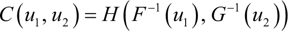
where F⁻¹(u₁) = x₁ and G⁻¹(u₂) = x₂ are the inverse distribution functions of the x₁ and x₂, respectively.

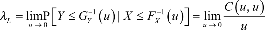
The upper coefficient measures the probability of observing extremely large value in x conditioned on the probability of observing such extremely large value in y. Similarly, the lower coefficient measures the probability of occurring extremely small value. These coefficients are determined by the following formula:

λ_{U} = \underset{u \to 1^{-}}{limP} [Y > G_{Y}^{- 1} (u) | X > F_{X}^{- 1} (u)] = \lim_{u \to 1} \frac{1 - 2 u + C (u, u)}{1 - u}

(5)

λ_{L} = \underset{u \to 0}{limP} [Y \leq G_{Y}^{- 1} (u) | X \leq F_{X}^{- 1} (u)] = \lim_{u \to 0} \frac{C (u, u)}{u}

(6)

Vine Copula

Vine copulas are a special case of modelling dependence for high dimensional probability distributions (Aas et al. 2009; Bedford & Cooke, 2001, 2002). Here, d-dimensional copulas are decomposed into conditional bivariate copulas such that there are d(d−1)/2 copula pairs in the d-linked tree (connected with notes and edges) and each pair copula can have multiple parameters.

Thus, vine copulas provide the advantages of multi-variate copulas function by separating the marginals from the dependence structure and the flexibility of bivariate copulas.

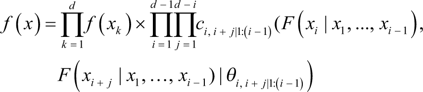
The joint density function of n RVs (X₁,…,X_n) can be represented by

f (x_{1}, \dots, x_{d}) = f (x_{d}) f (x_{d - 1} | x_{d}) f (x_{1} | x_{2}, \dots, x_{d})

(7)

where f (•│•) imply the conditional density.

Using Sklar’s theorem

f (x_{j} | v) = C_{(x_{j} v_{i} | v_{- i})} (F (x_{j} | v_{- i}), F (v_{i} | v_{- i})) f (x_{j} | v_{- i})

(8)

where v = {x_i_{+ 1, …,} x_d) is the conditioning set of marginal distribution of x_i, v_i represents ith component of the v vector and v_{– i} is the vector that excludes components v_i.

Since, the decomposition in Equation (7) is not unique, there can exist several ways to specify Pair Copula Construction (PCCs). This study adopted C-Vine decomposition and determines the sequence of the variables based on absolute value of Kendall’s tau. The star structure C-Vine is desirable where one variable is considered to be key one in influencing the relationship with the rest of the variables.

Further, graphs of four-dimensional C-Vine trees are shown in Figure 2.

Figure 2.

Graphical Representation of Four-Dimensional C-Vine Trees.

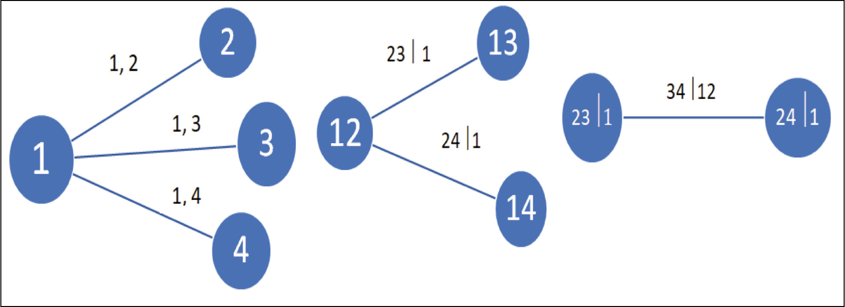
The sequence of variables is decided using Kendall’s tau. After deciding the arrangement of the variables in C-Vine structure, the best-fit copula family for each pair is chosen applying the information criterion namely AIC.

For estimating copula parameters two-step procedure known as Inference Function Margins (IFM) is applied, where first margins are non-parametrically transformed into uniform distribution using empirical cumulative distribution function (ECDF). Then C-Vine copula parameters are estimated using MLE. Vine parameters are typically estimated using a sequential method via maximum likelihood. However, results can be improved by estimating jointly using MLE taking starting values from the parameters estimated by the sequential method.

The C-Vine copula log-likelihood is defined as

\begin{array}{l} f (x) = \prod_{k = 1}^{d} f (x_{k}) \times \prod_{i = 1}^{d - 1} \prod_{j = 1}^{d - i} c_{i, i + j | 1 : (i - 1)} (F (x_{i} | x_{1}, ..., x_{i - 1}), \\ F (x_{i + j} | x_{1}, \dots, x_{i - 1}) | θ_{i, i + j | 1 : (i - 1)}) \end{array}

(9)

Results

Preliminary Results

Preliminary analysis and results are presented as follows:

Descriptive Statistics

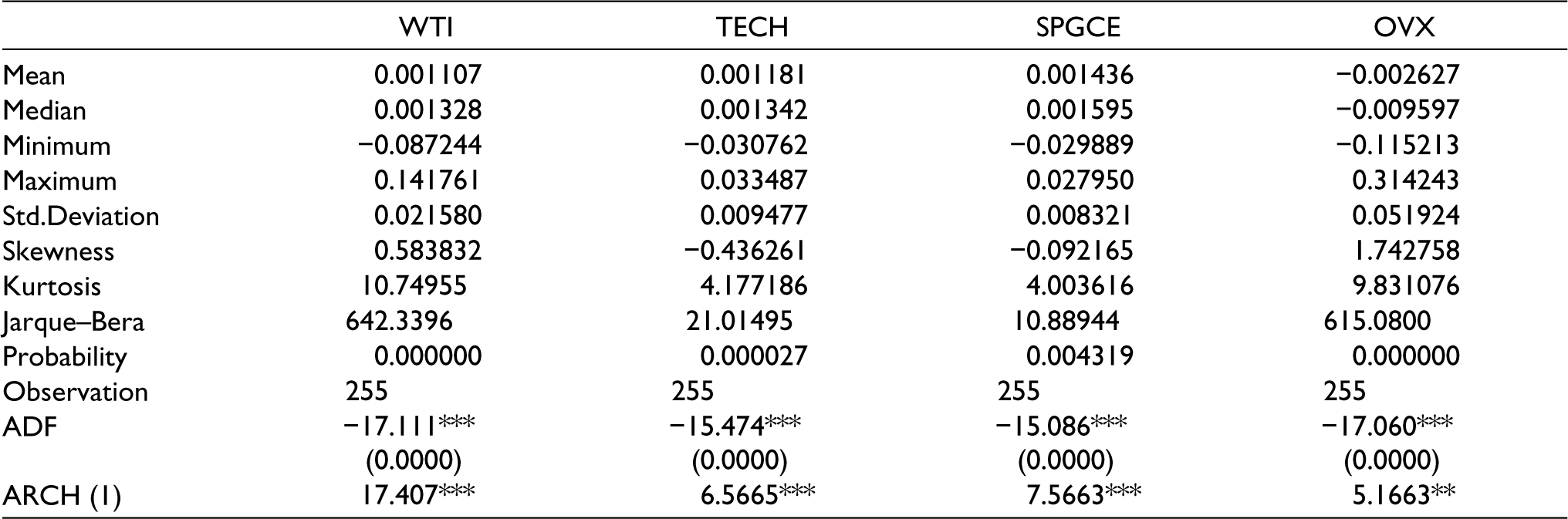
Descriptive statistics of Before-Covid period are put in Table 1.

Table 1.

Before-COVID Period.

	WTI	TECH	SPGCE	OVX
Mean	0.001107	0.001181	0.001436	−0.002627
Median	0.001328	0.001342	0.001595	−0.009597
Minimum	−0.087244	−0.030762	−0.029889	−0.115213
Maximum	0.141761	0.033487	0.027950	0.314243
Std.Deviation	0.021580	0.009477	0.008321	0.051924
Skewness	0.583832	−0.436261	−0.092165	1.742758
Kurtosis	10.74955	4.177186	4.003616	9.831076
Jarque–Bera	642.3396	21.01495	10.88944	615.0800
Probability	0.000000	0.000027	0.004319	0.000000
Observation	255	255	255	255
ADF	−17.111*** (0.0000)	−15.474*** (0.0000)	−15.086*** (0.0000)	−17.060*** (0.0000)
ARCH (1)	17.407***	6.5665***	7.5663***	5.1663**

Note: Statistical significance at the 0.01, 0.05 and 0.10 are indicated by the ***, ** and *, respectively.

Descriptive statistics of during–Covid period are put in Table 2.

Table 2.

During-COVID Period.

	WTI	TECH	SPGCE	OVX
Mean	−0.002371	0.000843	0.002284	0.001639
Median	0.000489	0.002579	0.004379	−0.009327
Minimum	−0.281382	−0.126212	−0.124971	−0.622251
Std.Deviation	16.51874	0.024737	0.027242	0.120676
Kurtosis	12.62424	8.538152	9.101443	21.15684
Jarque–Bera	69188.57	287.8327	348.8690	2740.264
Probability	0.00000	0.000000	0.00000	0.000000
Observation	192	192	192	192
ADF	−22.752***	–8.0575***	–8.11525**	–13.479***
ARCH (1)	3.7067**	6.6323***	7.5539***	1.3918

Note: Statistical significance at the 0.01, 0.05 and 0.10 are indicated by the ***, ** and *, respectively.

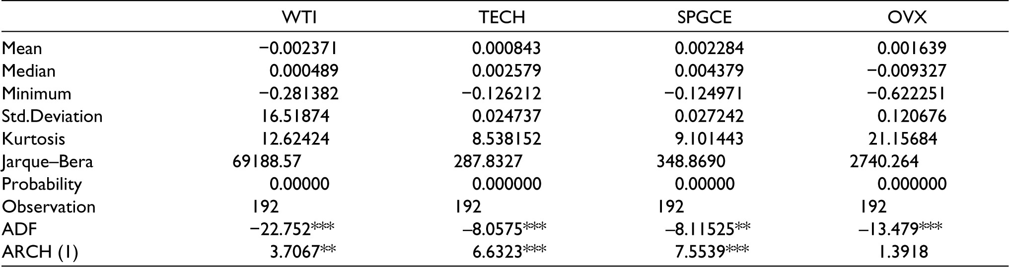
Table 1 summarizes the descriptive properties of the variables. All variables, except OVX (before-COVID) and WTI (during-COVID), have positive returns, although closer to zero. WTI observed drastic fall in the mean returns while SPGCE has shown higher mean return in the COVID period. OVX and WTI have the greatest volatility in the before and during COVID period, respectively.

The volatility of each variable has increased in the COVID period. The medians are not equal to mean returns exhibiting the non-normal distribution of the series. The maximum and minimum returns values of the WTI crude oil future in the COVID period exhibits the sudden disrupt in the oil prices due to COVID-19. All variables are somewhat asymmetric as shown by their non-zero skewness coefficients. The kurtosis coefficients for all the return series showed a strong departure from the normality, particularly fat tail behaviour. Further, the Jarque–Bera test (Jarque & Bera, 1987) also rejected the null hypothesis of a normal distribution. Besides, the ADF test rejected the null hypothesis of presence of unit root indicating all series are stationary at levels.

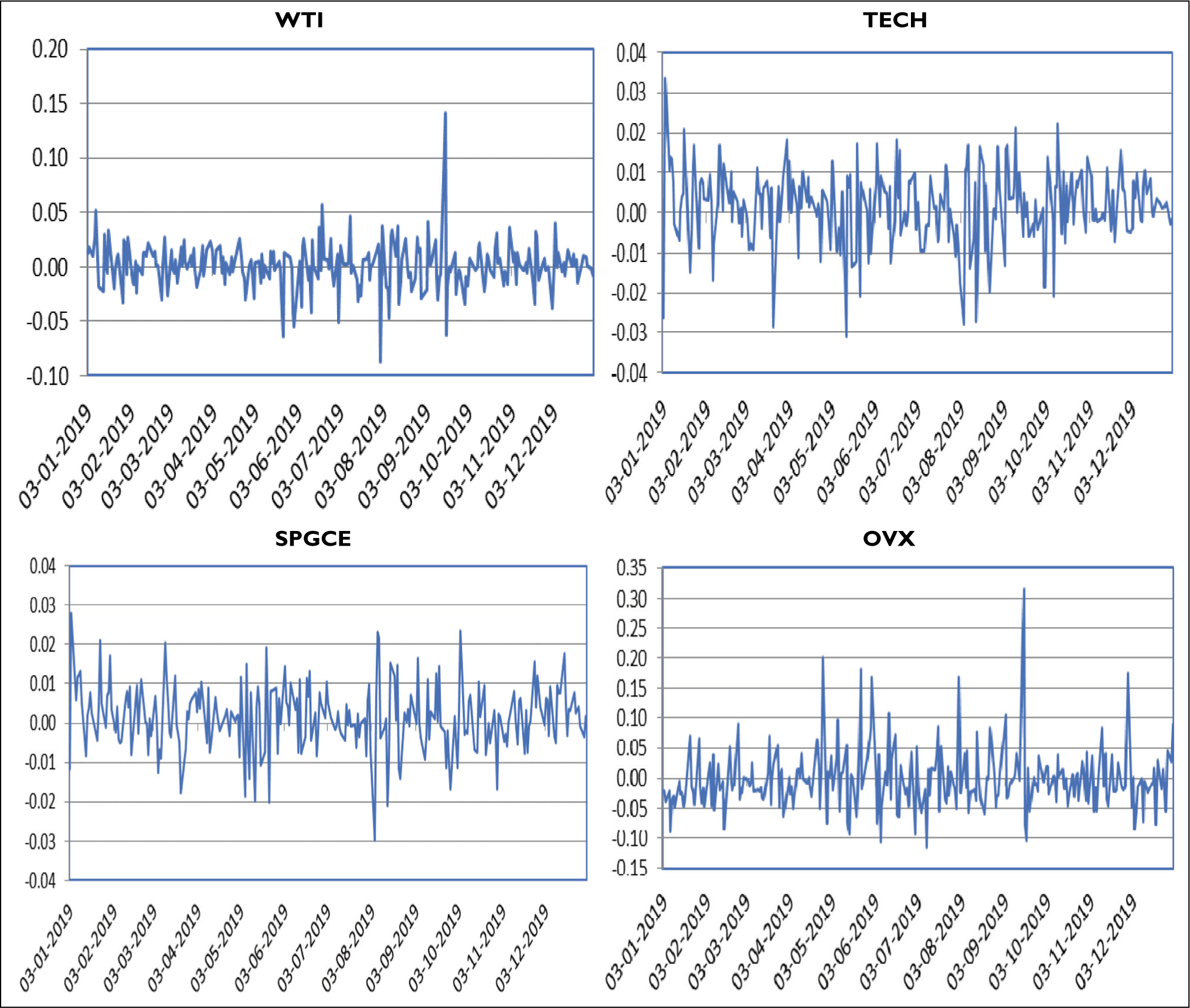
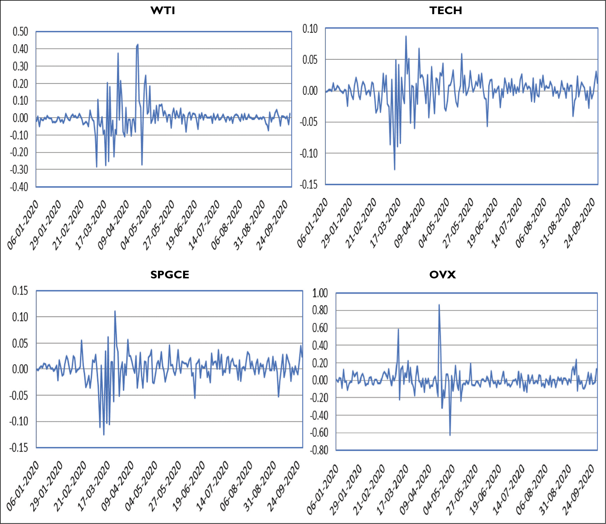
The log return series of the variables for before and during COVID periods are plotted in Figures 3 and 4, respectively. The graphs exhibit volatility clustering in the data and thus, GARCH model would be appropriate for modelling the return series. Moreover, the Engle-LM test found the presence of conditional heteroskedasticity in the series.

Figure 3.

Plots of the Return in the Before-COVID Period.

Figure 4.

Plots of the Return in the During COVID Period.

Empirical Results

Empirical analysis is presented as follows:

ARMA (p,q)-GARCH (1,1) Model

In this study, the ARMA-GARCH model is used to estimate the parameters of the marginals. The best-fitting model is selected among different lag orders (ARMA (0,0), ARMA (0,1), ARMA (1,0), ARMA (1,1)) with the error term following the normal, student’s t or Generalized Error Distribution (GED). The lag order for the ARMA model is specified based on the minimum value for the AIC.

The estimated parameters from the select models are reported in Table 3.

As shown in Tables 3 and 4, all the return series are best captured either by the GED or student-t distribution based on AIC. The Autoregressive and Moving Average (ARMA) terms are statistically significant for the select variables. The ARCH coefficients represented by α exhibit the influence of past squared residuals. On the other hand, GARCH coefficient represented by β shows the impact of lagged forecasted variance. The ARCH and GARCH coefficients are statistically significant at 1% for all series except for OVX (α is not statistically significant). Further, the sum of ARCH and GARCH coefficients is closer to unity signify that the shocks are persistent. The Shape parameters are statistically significant indicating that the return series were asymmetrically distributed.

Lastly, the residuals diagnostic results are also reported in Tables 3 and 4. We used ARCH LM test and Ljung-Box statistics for standardized residuals as well as standardized squared residuals by applying different lag structures.

Table 3.

ARMA (p,q)-GARCH (1,1) Model.

	Before-COVID Period (1st January 2019–4th January 2020)
	WTI	TECH	SPGCE	OVX
	GED	Student t	GED	Student t
c	0.001408*** [0.000252]	0.001511*** [0.000517]	0.001419*** [0.000492]	−0.00877*** [0.002104]
φ	–	–	−0.84539 [0.057008]	–
θ	−0.041685*** [0.014787]	–	0.928443*** [0.036646]	0.162283*** [0.045460]
ω	0.000014*** [0.00003]	0.00006* [0.00003]	0.00009*** [0.00001]	0.000131 [0.000152]
α	0.042624*** [0.010311]	0.12906*** [0.041609]	0.12284*** [0.035893]	0.022272 [0.022057]
β	0.923507*** [0.022093]	0.805598*** 0.048760]	0.74492***1 [0.052650]	0.937593*** [0.056653]
Shape	1.020203*** [0.104693]	7.783721*** [3.001746]	1.447011*** [0.179497]	2.955765*** [0.530233]
Diagnostic Tests ARCH LM Test
ARCH (3)	0.7412	0.08227*	0.07073*	0.7229
ARCH (5)	0.9750	0.21594	0.22548	0.9387
ARCH (7)	0.9968	0.43928	0.6749	0.9872
Ljung-Box on Standardized Residuals
L-B (1)	0.4757	0.1274	0.1325	0.8790
L-B (5)	0.9622	0.1073	0.2188	1.000
L-B (9)	0.7682	0.1519	0.3112	0.9999
Ljung-Box on Squared Standardized Residuals
L-B² (1)	0.2001	0.6201	0.6984	0.3122
L-B² (5)	0.6631	0.5621	0.5062	0.8068
L-B² (9)	0.9162	0.7473	0.6754	0.8402

Note: Statistical significance at the 0.01, 0.05 and 0.10 are indicated by the ***, ** and *, respectively. Standard errors are shown in parentheses [ ].

Table 4.

ARMA (p,q)-GARCH (1,1) Model.

	During-COVID Period (5th January 2020–31st September 2020)
	WTI	TECH	SPGCE	OVX
	GED	Student t	Student t	Student t
c	0.00189*** [0.00014]	0.002828*** [0.00100]	0.004702*** [0.00122]	−0.00954** [0.004694]
φ	−0.48987*** [0.013173]	−0.057388** [0.279194]	–	−0.89592*** [0.112979]
θ	0.373285*** [0.011096]	0.5224481* [0.285613]	–	0.913523*** [0.099002]
ω	0.00014* [0.000086]	0.00002 [0.000015]	0.000042 [0.000029]	0.002098 [0.002426]
α	0.434716*** [0.124046]	0.198097** [0.082249]	0.226334* [0.118979]	0.271433 [0.294528]
β	0.564284*** [0.106672]	0.800903*** [0.078796]	0.772666*** [0.095075]	0.702861*** [0.112281]
Shape	0.785133*** [0.090157]	3.706122*** [1.207001]	3.569544** [1.443933]	2.548796*** [0.742471]
Diagnostic Tests ARCH LM Tests
ARCH (3)	0.7412	0.08227	0.07073	0.7229
ARCH (5)	0.9750	0.21594	0.22548	0.9387
ARCH (7)	0.9968	0.43928	0.6749	0.9872
Ljung-Box on Standardized Residuals
L-B (1)	0.4757	0.1274	0.1325	0.8790
L-B (5)	0.9622	0.1073	0.2188	1.000
L-B (9)	0.7682	0.1519	0.3112	0.9999
Ljung-Box on Squared Standardized Residuals
L-B² (1)	0.2001	0.6201	0.6984	0.3122
L-B² (5)	0.6631	0.5621	0.5062	0.8068
L-B² (9)	0.9162	0.7473	0.6754	0.8402

Note: Statistical significance at the 0.01, 0.05 and 0.10 are indicated by the ***, ** and *, respectively. Standard errors are shown in parentheses [ ].

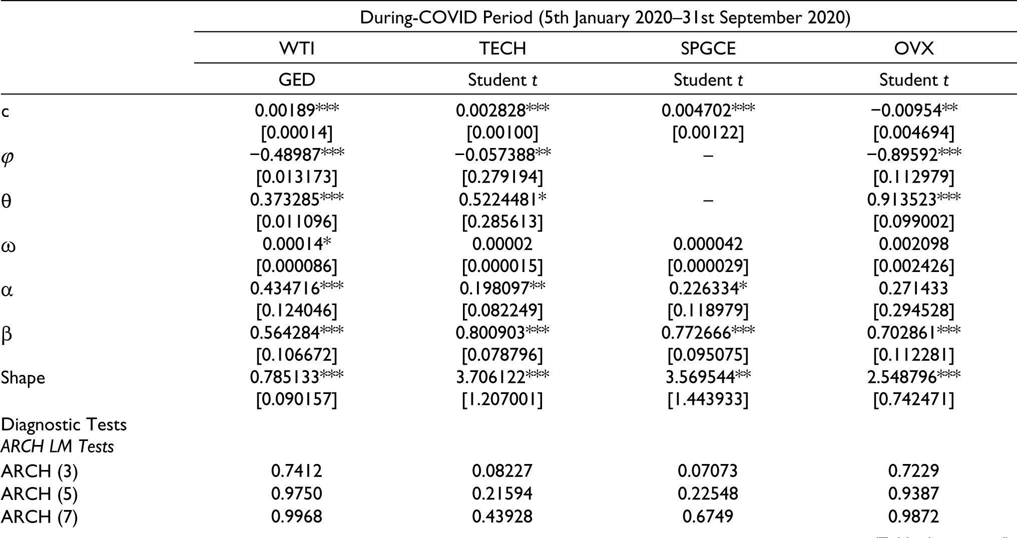
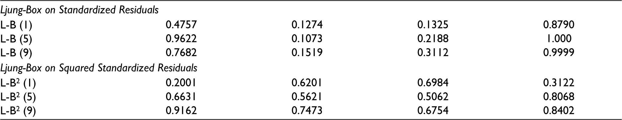
We conclude from the results of ARCH LM test that there is an absence of conditional heteroscedasticity in the series for the different specification of ARCH lags. Moreover, the significance results of Ljung-Box on statistics on standardized residuals as well as standardized squared residuals reported that there is an absence of serial correlation in the series.

The diagnostic check on residuals is very crucial step in the marginal modelling as copula analysis requires the observations to be i.i.d. (Independent and Identically Distributed). The presence of autocorrelation and heteroscedasticity in the standardized residuals may produce statistical biasness in the copula results. The standardized residuals from the GARCH models are employed for the copula modelling.

Different copula families are used to studying the dependence between the variables. Therefore, standard residuals from the GARCH models are transformed into uniform distribution using Empirical Cumulative Distribution Function.

The next step is to identify the sequence of the variables in the C-Vine structure. In this study, WTI is placed at the first place in the order of the variables. For the rest of the variables, this study has used the method proposed by Czado et al. (2012) for identifying the maximal tree spanning by arranging the variables in accordance to their sum of absolute pairwise estimated Kendall’s tau │The variable with the highest dependency is placed at the next sequence and so on.

By this method, the order of the variable is decided as WTI, TECH, SPGCE and OVX. This sequence applies to the before and during COVID periods in both datasets.

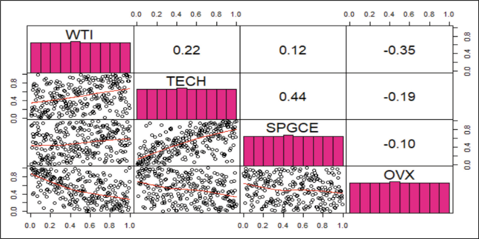
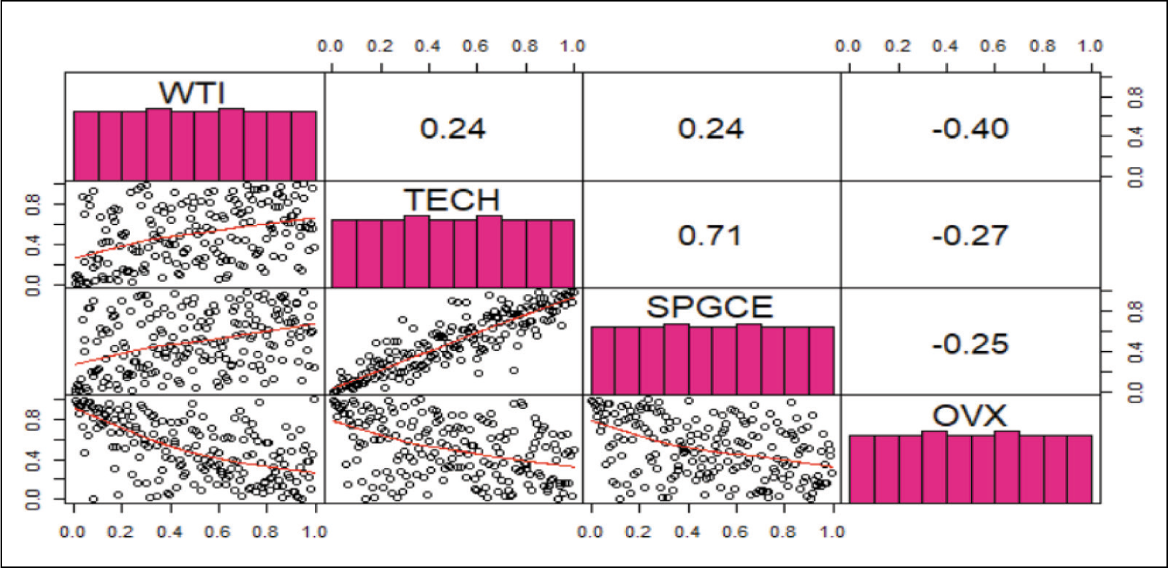
Figures 5 and 6 show Kendall’s τ (above the diagonal) and pairwise scatter plot (below the diagonal) of the copula data. From the graph, it is evident that renewable energy indices have strong dependence while OVX has rather weak dependence with other indices. From the estimated Kendall’s τ, TECH is the highest dependent variable with the rest of the variables as it has the greatest sum of Kendall’s tau, which labels it as the second variable followed by SPGCE and OVX for C-Vine decomposition.

Figure 5.

Kendall’s τ and Scatter Plot for the Before COVID Period.

Figure 6.

Kendall’s τ and Scatter Plot for the COVID Period.

C-Vine Copula

Estimates of Vine Copula are given as follows:

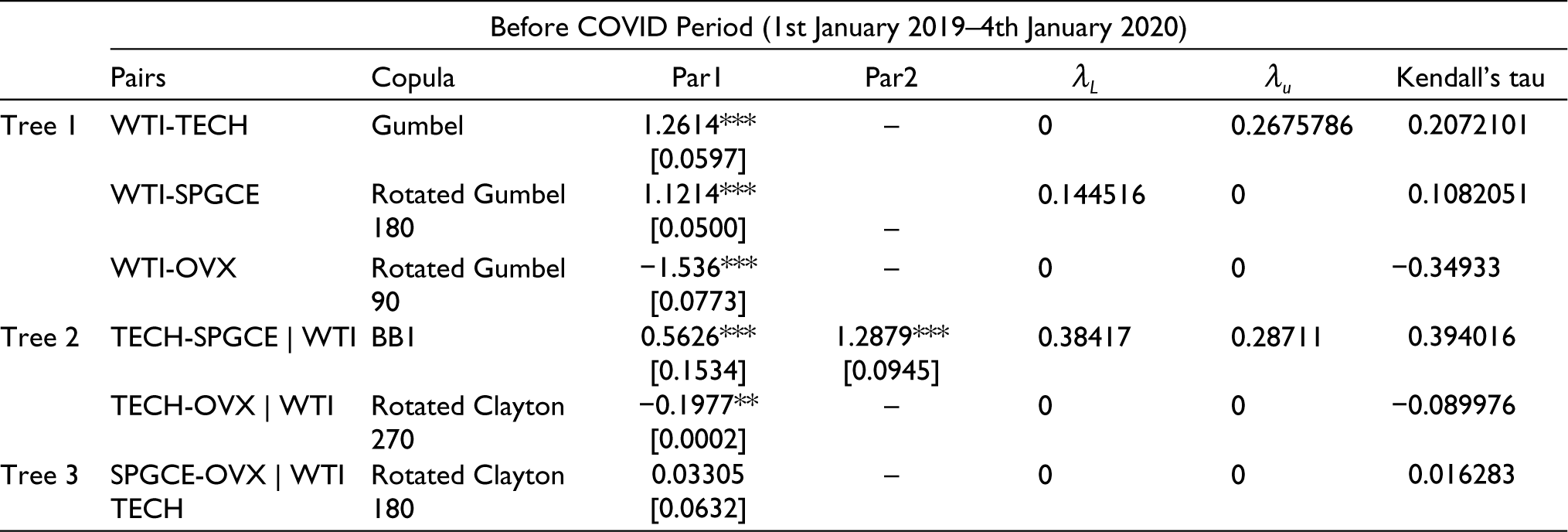
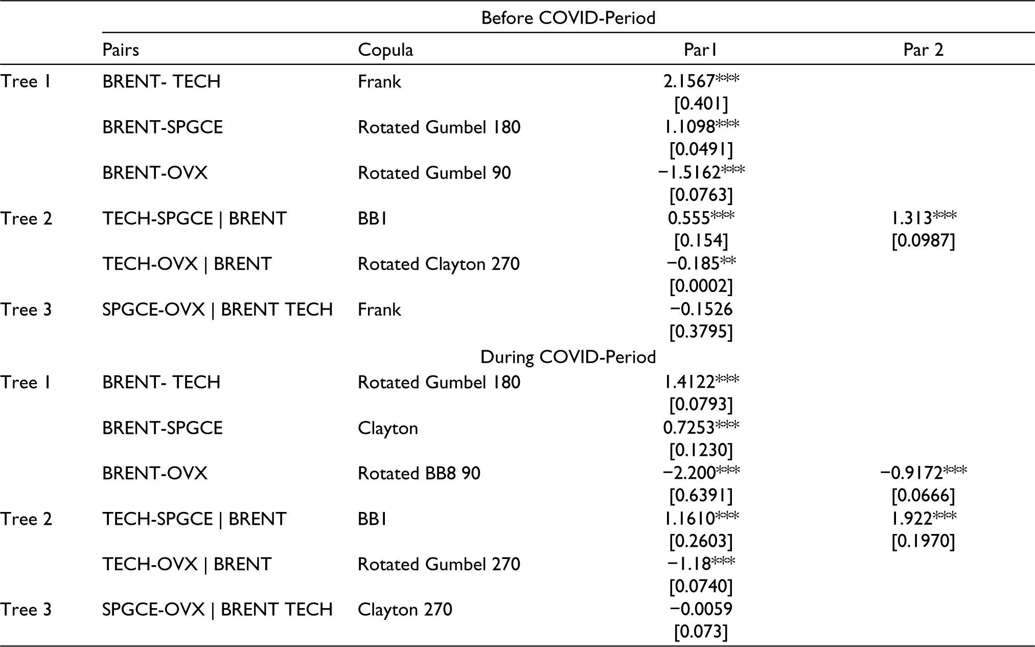
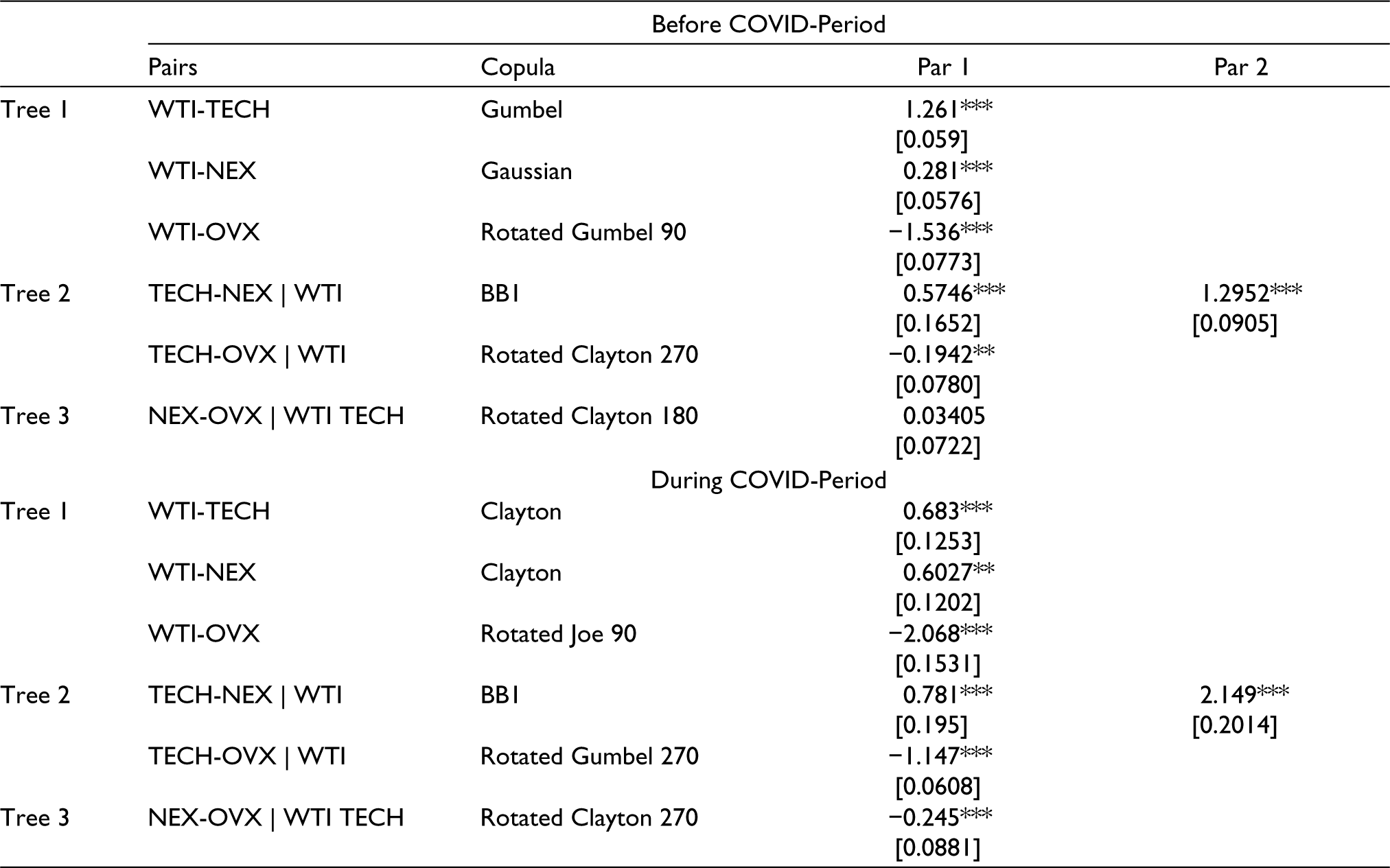
The next step involves choosing a suitable copula family model for each pair and estimating their parameters accordingly. Gumbel, Rotated Gumbel 180, Rotated Gumbel 90, BB1, Rotated Clayton 270, and Rotated Clayton 180 copula models are chosen for before-COVID-19 period. Besides, Clayton, Rotated BB8 90, BB1, Rotated Gumbel 270 and Gaussian copula models are chosen for during-COVID-19 period.

Tables 5 and 6 summarize the results of parameters estimated for the C-Vine copula structure. The first tree reflects the degree and structure of dependence between WTI and three other indices—TECH, SPGCE and OVX. The estimated Kendall’s tau provides evidence that the degree of dependence has increased between WTI and other three indices in the COVID period. This implies that SPGCE and TECH are more positively correlated with the movements in the returns of WTI. The dependence structure between WTI and SPGCE is shifted from rotated Gumbel 180° to Clayton copula. Both the copulas measure the lower tail dependence suggesting that downward movements in the index’s returns are more correlated than upward movements. The positive co-movement in the downside movements imply that reducing oil price could make renewable energy less competitive. For instance, the oil prices fell below $22.58 amid the coronavirus pandemic, the cheap availability of the oil reduces the appetite for renewable energy. This higher positive dependency in the lower region either exhibit the presence of substitution effect or impact of lockdown which reduces the demand for both oil and renewable energy.

Before-Covid estimations are given in Table 5.

Table 5.

Estimation of Four-dimensional C-Vine Copula.

	Before COVID Period (1st January 2019–4th January 2020)
	Pairs	Copula	Par1	Par2	λ_L	λ_u	Kendall’s tau
Tree 1	WTI-TECH	Gumbel	1.2614*** [0.0597]	–	0	0.2675786	0.2072101
	WTI-SPGCE	Rotated Gumbel 180	1.1214*** [0.0500]	–	0.144516	0	0.1082051
	WTI-OVX	Rotated Gumbel 90	−1.536*** [0.0773]	–	0	0	−0.34933
Tree 2	TECH-SPGCE \| WTI	BB1	0.5626*** [0.1534]	1.2879*** [0.0945]	0.38417	0.28711	0.394016
	TECH-OVX \| WTI	Rotated Clayton 270	−0.1977** [0.0002]	–	0	0	−0.089976
Tree 3	SPGCE-OVX \| WTI TECH	Rotated Clayton 180	0.03305 [0.0632]	–	0	0	0.016283

Note: Statistical significance at the 0.01, 0.05 and 0.10 are indicated by the ***, ** and *, respectively. Standard errors are shown in parentheses [ ].

During-Covid Estimations are given in Table 6.

Table 6.

Estimation of Four-dimensional C-Vine Copula.

	During COVID Period (5th January 2020–31st September 2020)
	Pairs	Copula	Par1	Par 2	λ_L	λ_u	Kendall’ tau
Tree 1	WTI-TECH	Clayton	0.688*** [0.1021]	–	0.362625	0	0.254654
	WTI-SPGCE	Clayton	0.658*** [0.1060]	–	0.349076	0	0.247723
	WTI-OVX	Rotated BB8 90	−2.40*** [0.0989]	–0.967*** [0.0065]	0	0	−0.39938
Tree 2	TECH-SPGCE \| WTI	BB1	0.988*** [0.2700]	2.016*** [0.2287]	0.706337	0.58987	0.668180
	TECH-OVX \| WTI	Rotated Gumbel 270	−1.16*** [0.0736]	0	0	0	−0.13990
Tree 3	SPGCE-OVX \| WTI TECH	Gaussian	−0.0546 [0.0721]	0	0	0	−0.03474

Note: Statistical significance at the 0.01, 0.05 and 0.10 are indicated by the ***, ** and *, respectively. Standard errors are shown in parentheses [ ].

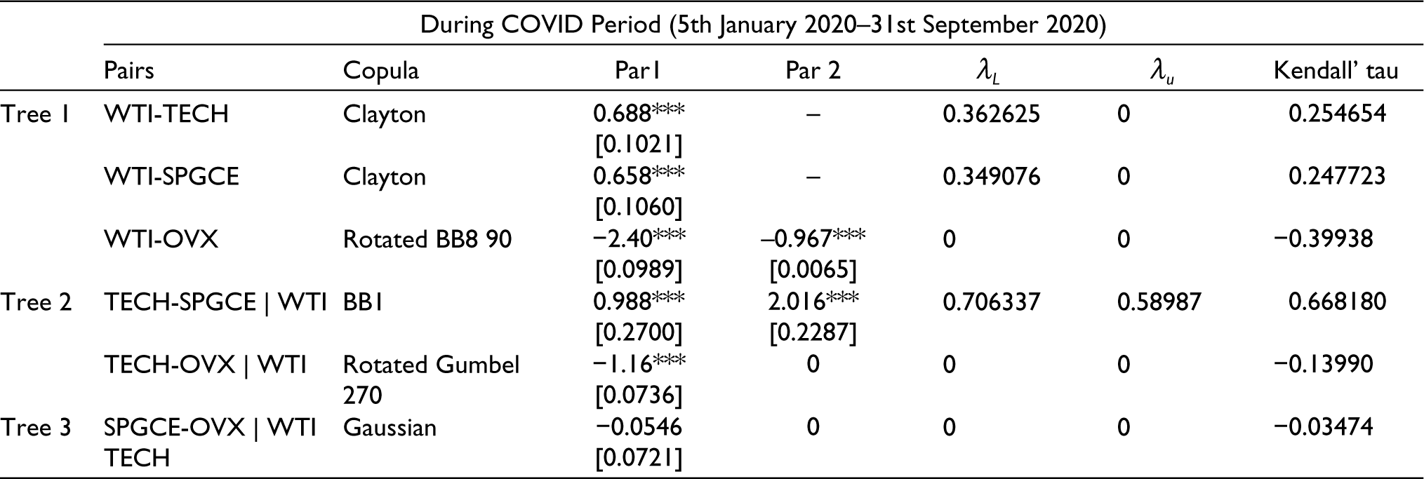
Further, the positive association between WTI and TECH accelerated, however, the dependence structure changed from Gumbel copula which exhibits right tail dependence to Clayton copula which exhibits left tail dependence. This left tail (lower-lower) dependence between WTI and TECH indicates that both are bearish during COVID-19 period.

The dominance of lower-lower dependence can be attributed to the looming economies across the globe due to lockdown. The low oil prices could not stimulate the demand for new investments in clean energy technology. Further, the degree of a negative association between WTI and OVX increased as indicated by the value of Kendall’s tau. As for the dependence structure, the fitted pair copula families are rotated Gumbel 90 and Rotated BB8 90 copulas in the before and during COVID periods, respectively. The paired variables before COVID-19 have an asymmetrical dependence but turns symmetrical during COVID-19 period. More noticeably, WTI crude oil appears to have strongest connection with OVX rather than SPGCE and TECH.

Next, in the second tree, we explored the dependence between TECH, SPGCE and OVX conditional on WTI. Given the returns of WTI, the value of Kendall’s tau between TECH and SPGCE increased by a great margin in the COVID period. Also, the dependence degree of TECH and SPGCE is the highest among all the pairs. This implies that returns of SPGCE are more relevant to the TECH than WTI advocating that TECH is an important variable to give a boost to the global energy transition. The dependence structure is the same between both the periods, modelled through BB1 copula. This copula measures asymmetrical co-movements such as extreme losses are more correlated than extreme gains.

Furthermore, conditioned on WTI, the TECH and OVX had a negative degree of dependence with higher dependence in the COVID period. The joint distribution here is best described by 270 rotated Clayton and Gumbel copulas which show the existence of negative dependence in the upper-lower region in the before and during COVID period, respectively. The negative dependence is relatively obvious as it implies that technology sector does not perform well in the period of higher volatility in oil prices (in the COVID period) and vice-versa (Sadorsky, 2003).

Lastly, in the third tree, the dependence between SPGCE and OVX is measured through conditional on the returns of WTI and TECH. Firstly, the lowest Kendall’s tau between SPGCE and OVX signals that SPGCE returns are highly influenced by the WTI and TECH rather than the OVX.

The magnitude of the dependence is very less but it changed from positive to negative association, although copula parameters are not significant in both the periods. The insignificant linkage would allow the investors to diversify the risk by including renewable energy stocks and OVX in their energy portfolio.

As for the dependence structure, the Rotated Clayton 180 suggests that their extremely negative returns are correlated before COVID-19 but it changed to symmetric dependence as indicated by the best fit of Gaussian copula in the COVID period. This dependence structure indicates that tail dependence between SPGCE AND OVX is relatively weak and has no asymmetry.

Robustness Analysis

This section checks the robustness of our results by using alternative GARCH-type models and employing different indices of oil prices and renewable energy stock. This procedure is important as it confirms the suitability of our proposed approach for examining the relationship between oil and renewable energy.

Alternative GARCH-type Models

The standard GARCH model takes into consideration serial dependence and volatility clustering but does not capture leverage and long memory effect. The oil and renewable energy index may exhibit these effects in conditional variance. If these effects are present in the time series, then, marginal specifications based on ARMA-GARCH (1,1) model may not be appropriate. Hence, we consider alternative GARCH models namely, Exponential GARCH (EGARCH) and Fractional Integrated GARCH (FIGARCH) to capture leverage and long-memory effects. Tables 7 and 8 reported the best-fitted copula chosen under the alternative GARCH models. Overall, the best-fitted copula chosen by the alternative GARCH specifications are majorly similar to the copula models selected by the initial GARCH specifications in both the periods. The value of coefficients also does not vary much from the findings in Tables 5 and 6.

Table 7.

Estimation of Copula Parameters with EGARCH Marginal Specifications.

	Before COVID-Period
	Pairs	Copula	Par1	Par 2
Tree 1	WTI-TECH	Gumbel	1.2650*** [0.0601]
	WTI-SPGCE	Rotated Gumbel 180	1.1376*** [0.0513]
	WTI-OVX	Rotated Gumbel 90	−1.516*** [0.0763]
Tree 2	TECH-SPGCE \| WTI	BB1	0.4952** [2.520]	1.636*** [0.227]
	TECH-OVX \| WTI	Rotated BB8	−0.2175*** [0.0795]
Tree 3	SPGCE-OVX \| WTI TECH	Rotated Joe	1.0233 [0.0392]
	During COVID-Period
Tree 1	WTI-TECH	Clayton	0.668*** [0.1123]
	WTI-SPGCE	Clayton	0.638*** [0.1120]
	WTI-OVX	Rotated BB8 90	−2.29*** [0.0100]	−0.917*** [0.0666]
Tree 2	TECH-SPGCE \| WTI	Rotated Gumbel 180	3.0089*** [0.1795]	1.922*** [0.1970]
	TECH-OVX \| WTI	Rotated Gumbel 270	−1.1852** [0.053]
Tree 3	SPGCE-OVX \| WTI TECH	Rotated Clayton 90	0.0468 [0.0721]

Note: Statistical significance are indicated by the *, **, *** at the 0.01, 0.05 and 0.10 levels, respectively. Standard errors are shown in square brackets.

Table 8.

Estimation of Copula Parameters with FIGARCH Marginal Specifications.

	Before COVID-Period
	Pairs	Copula	Par1	Par 2
Tree 1	WTI-TECH	Gumbel	1.3018*** [0.0852]
	WTI-SPGCE	Frank	1.0755*** [0.3886]
	WTI-OVX	Rotated Gumbel 90	−1.5214*** [0.0764]
Tree 2	TECH-SPGCE \| WTI	BB1	0.547*** [0.1531]	1.319*** [0.0995]
	TECH-OVX \| WTI	Gaussian	−0.1850** [0.0610]
Tree 3	SPGCE-OVX \| WTI TECH	Rotated Clayton 180	0.0370 [0.0640]
	During COVID-Period
Tree 1	WTI-TECH	Clayton	0.642*** [0.1233]
	WTI-SPGCE	Clayton	0.690*** [0.1295]
	WTI-OVX	Rotated BB8 90	−2.20*** [0.1100]	−0.852*** [0.0036]
Tree 2	TECH-SPGCE \| WTI	BB1	0.882*** [0.3600]	2.502*** [0.1982]
	TECH-OVX \| WTI	Rotated Gumbel 270	−1.18*** [0.0752]
Tree 3	SPGCE-OVX \| WTI TECH	Rotated Clayton 90	0.0468 [0.0721]

Note: Statistical significance are indicated by the *, **, *** at the 0.01, 0.05 and 0.10 levels, respectively. Standard errors are shown in square brackets.

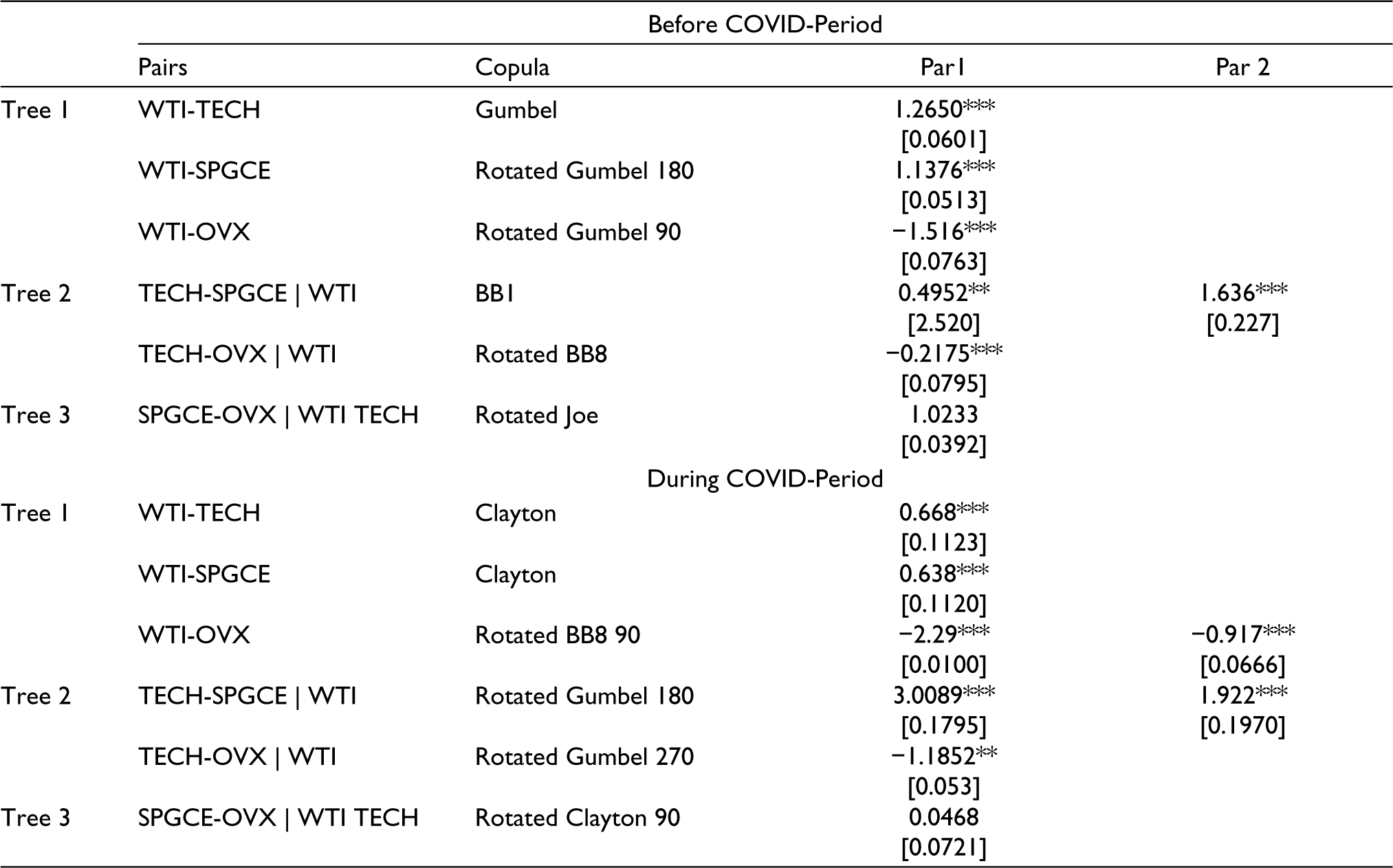
Alternative Oil and Renewable Energy Indices

It will be also interesting to know how our previous results will change when we employ different indices of oil price and renewable energy stock returns. To do so, we estimate the copula models with Brent oil futures replacing WTI oil futures and WilderHill Clean Energy Index (NEX) replacing SPGCE index. Table 9 reports the results of best-fitted copula and estimated parameters when brent oil returns are used. Overall, the findings are similar to those we obtained when using WTI crude oil. First, out of the six copula models in each period, five are statistically significant in the before and during COVID-period. Second, similar copula families are chosen for the four pairs and the value of coefficients are very close to the initial results.

Table 9.

Estimation of Copula Parameters with Brent Oil Prices.

	Before COVID-Period
	Pairs	Copula	Par1	Par 2
Tree 1	BRENT- TECH	Frank	2.1567*** [0.401]
	BRENT-SPGCE	Rotated Gumbel 180	1.1098*** [0.0491]
	BRENT-OVX	Rotated Gumbel 90	−1.5162*** [0.0763]
Tree 2	TECH-SPGCE \| BRENT	BB1	0.555*** [0.154]	1.313*** [0.0987]
	TECH-OVX \| BRENT	Rotated Clayton 270	−0.185** [0.0002]
Tree 3	SPGCE-OVX \| BRENT TECH	Frank	−0.1526 [0.3795]
	During COVID-Period
Tree 1	BRENT- TECH	Rotated Gumbel 180	1.4122*** [0.0793]
	BRENT-SPGCE	Clayton	0.7253*** [0.1230]
	BRENT-OVX	Rotated BB8 90	−2.200*** [0.6391]	−0.9172*** [0.0666]
Tree 2	TECH-SPGCE \| BRENT	BB1	1.1610*** [0.2603]	1.922*** [0.1970]
	TECH-OVX \| BRENT	Rotated Gumbel 270	−1.18*** [0.0740]
Tree 3	SPGCE-OVX \| BRENT TECH	Clayton 270	−0.0059 [0.073]

Note: Statistical significance are indicated by the *, **, *** at the 0.01, 0.05 and 0.10 levels, respectively. Standard errors are shown in square brackets.

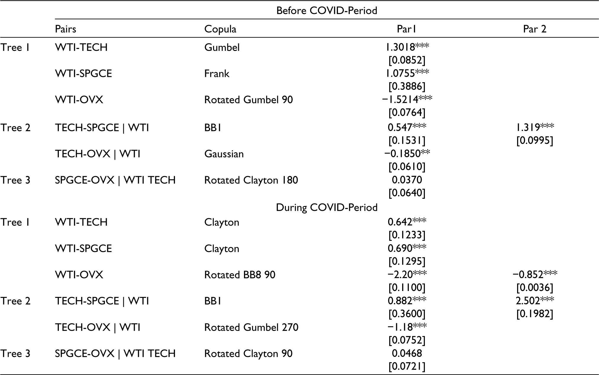
Next, we estimate the copula models with NEX replacing SPGCE index (Table 10). Majority of the pairs selected similar copula models as we observed in Tables 5 and 6 for the both the periods. Moreover, the value of coefficients does not differ from the results presented previously.

Table 10.

Estimation of Copula Parameters with NEX.

	Before COVID-Period
	Pairs	Copula	Par 1	Par 2
Tree 1	WTI-TECH	Gumbel	1.261*** [0.059]
	WTI-NEX	Gaussian	0.281*** [0.0576]
	WTI-OVX	Rotated Gumbel 90	−1.536*** [0.0773]
Tree 2	TECH-NEX \| WTI	BB1	0.5746*** [0.1652]	1.2952*** [0.0905]
	TECH-OVX \| WTI	Rotated Clayton 270	−0.1942** [0.0780]
Tree 3	NEX-OVX \| WTI TECH	Rotated Clayton 180	0.03405 [0.0722]
	During COVID-Period
Tree 1	WTI-TECH	Clayton	0.683*** [0.1253]
	WTI-NEX	Clayton	0.6027** [0.1202]
	WTI-OVX	Rotated Joe 90	−2.068*** [0.1531]
Tree 2	TECH-NEX \| WTI	BB1	0.781*** [0.195]	2.149*** [0.2014]
	TECH-OVX \| WTI	Rotated Gumbel 270	−1.147*** [0.0608]
Tree 3	NEX-OVX \| WTI TECH	Rotated Clayton 270	−0.245*** [0.0881]

Note: Statistical significance are indicated by the *, **, *** at the 0.01, 0.05 and 0.10 levels, respectively. Standard errors are shown in square brackets.

Conclusion

In the past few years, researchers have extensively focused on analysing the nexus between WTI crude oil and renewable energy stock, but because of COVID-19 pandemic, this topic has become more intriguing.

This study analyses the dependency structure between WTI crude oil futures, two renewable energy indices CLEANTECH and SPGCE and oil price uncertainty index. It attempted to identify the change in their relationship after the outbreak of the COVID-19. The analysis was done using ARMA (p,q)-GARCH (1,1) with normal, student-t or generalized error distribution to model the return series. Thereafter, the copula model is applied to capture the dependence between variables and pairwise construction is done using C-Vine decompositions.

The empirical results showed the degree of dependence of WTI with SPGCE, TECH and OVX has increased during the COVID-19 period. Further, asymmetrical dependence structure exists between WTI and SPGCE before and during COVID-19 period. The increased positive association in the downside movement between WTI and SPGCE could imply the substitution effect between crude oil and renewable energy during COVID-19. Renewable energy requires huge investment, any considerable drop in the WTI oil price will only make renewable energy less competitive. Secondly, this dependence structure could also be explained by the fact that lockdown measures across the world would have wiped the energy demand globally and thus co-movement in the lower region.

The dependence structure between WTI and TECH changes from upper tail to lower dependence, highlighting the impact of lockdown across the globe. The technology sector is highly sensitive to the business cycle period; thus, the low economic activities could not stimulate the TECH returns although oil prices reduced notably. Besides, WTI crude oil appears to have strongest connection with OVX rather than SPGCE and TECH.

In the second tree, the results suggested that SPGCE is more influenced by TECH rather than WTI and OVX particularly in the COVID period. This finding corroborates with the previous researches of Ahmad (2017) and Kumar et al. (2012) that technology is an important variable to give a boost to the global energy transition.

The degree of dependence between SPGCE and OVX changes from positive to negative association. Although, insignificant linkages in both the periods implies that renewable energy does offer the benefit of diversifying an energy portfolio against the oil price uncertainty index.

Finally, our results are robust to the choice to alternative GARCH-type specifications allowing for leverage and long memory effects in the conditional volatility as well as choice to consider alternative indices for oil and renewable energy.

Policy Recommendations

The findings of this study have significant implications for policy-makers and investors in the energy market. The results imply that fluctuation in traditional energy prices is not the primary factor in the volatility of renewable energy stock price. In fact, technology played the central role in the price discovery of renewable energy and hence, there should be more subsidies allocated to the clean energy technology. This will reduce the clean energy production cost and will protect the clean energy technology stock against the oil prices fluctuations also.

Also, the findings have shown that huge drop in the oil prices after the outbreak of COVID- pandemic could make the transition to environmentally friendly energy sources more difficult. The imposition of fossil fuel and carbon tax can help in reducing the investment risk for the renewable energy sector.

In addition, our study has important implication for portfolio managers and investors. Findings indicate the scope of diversification by including OVX in the energy portfolio. The detachment of OVX and renewable energy in the turmoil period (during COVID) makes the investments in these assets more appealing.

These findings provide short-run insight on oil-renewable energy nexus. The long-term implication depends on the speed of economic recovery which will future determine the renewable energy investment. The future policies should encourage investment in clean energy projects to combat the negative implications of COVID-19.

Footnotes

Declaration of Conflicting Interests

The authors declared no potential conflicts of interest with respect to the research, authorship and/or publication of this article.

Funding

The authors received no financial support for the research, authorship and/or publication of this article.

Notes

References

Aas

, Czado

, Frigessi

, & Bakken

(2009). Pair-copula constructions of multiple dependence. Insurance: Mathematics and Economics, 44(2), 182–198.

Ahmad

(2017). On the dynamic dependence and investment performance of crude oil and clean energy stocks. Research in International Business and Finance, 42, 376–389.

Ahmad

, & Rais

(2018). Time-varying spill over and the portfolio diversification: Implications of clean energy equity with commodities and financial assets. Emerging Markets Finance and Trade, 54(8), 1837–1855.

Barunik

, & Krehlik

(2018). Measuring the frequency dynamics of financial connectedness and systemic risk. Journal of Financial Econometrics, 16(2), 271–296.

Bedford

, & Cooke

R. M.

(2001). Probability density decomposition for conditionally dependent random variables modelled by vines. Annals of Mathematics and Artificial Intelligence, 32(1), 245–268.

Bedford

, & Cooke

R. M.

(2002). Vines—A new graphical model for dependent random variables. The Annals of Statistics, 30(4), 1031–1068.

Ben

S. A.

(2015). The frequency of regime switching in financial market volatility. Journal of Empirical Finance, 32, 63–79.

Bondia

, Ghosh

, & Kanjilal

(2016). International crude oil prices and the stock prices of clean energy and technology companies: evidence from non-linear cointegration tests with unknown structural breaks. Energy, 101, 558–565.

Celik

İ.

, Sak

A. F.

, Höl

A. Ö.

, & Vergili

(2022). The dynamic connectedness and hedging opportunities of implied and realized volatility: Evidence from clean energy etfs. The North American Journal of Economics and Finance, 60, 101670. 10.1016/j.najef.2022.101670

10.

Choi

(2014). Causality test between investor’s sentiment and price movements: A case study of the NYMEX crude oil futures market. International Journal of Oil, Gas and Coal Technology, 7(3), 229.

11.

Czado

, Schepsmeier

, & Min

(2012). Maximum likelihood estimation of mixed C-vines with application to exchange rates. Statistical Modelling: An International Journal, 12(3), 229–255.

12.

De Blasis

, & Petroni

(2021). Price leadership and volatility linkages between oil and renewable energy firms during the COVID-19 pandemic. Energies, 14(9), 2608

13.

Diebold

F. X.

, & Yilmaz

(2012). Better to give than to receive: Predictive directional measurement of volatility spillovers. International Journal of Forecasting, 28(1), 57–66.

14.

Dutta

(2017). Oil price uncertainty and clean energy stock returns: new evidence from crude oil volatility index. Journal of Cleaner Production, 164, 1157–1166.

15.

Dutta

, Jana

R. K.

, & Das

(2020). Do green investments react to oil price shocks? Implications for sustainable development. Journal of Cleaner Production, 266,1–8.

16.

Ferrer

, Shahzad

S. J.

, Lopez

, & Jareno

(2018). Time and frequency dynamics of connectedness between renewable energy stocks and crude oil prices. Energy Economics, 76, 1–20.

17.

Geng

J.-B.

, Liu

, Ji

, & Zhang

(2021). Do oil price changes really matter for clean energy returns? Renewable and Sustainable Energy Reviews, 150, 111429.

18.

Ghabri

, Ayadi

, & Guesmi

(2021). Fossil energy and clean energy stock markets under COVID-19 pandemic. Applied Economics, 53(43), 4962–4974. 10.1080/00036846.2021.1912284

19.

Guo

, Yu

, Zhang

, & Cheng

(2021). Asymmetric between oil prices and renewable energy consumption in the G7 countries. Energy, 226, 120319. 10.1016/j.energy.2021.120319

20.

Hammoudeh

, Mokni

, Ben-Salha

, & Ajmi

A. N.

(2021). Distributional predictability between oil prices and renewable energy stocks: Is there a role for the COVID-19 pandemic? Energy Economics, 103, 105512.

21.

Jarque

C. M.

, & Bera

A. K.

(1987). A test for normality of observations and regression residuals. International Statistical Review/Revue Internationale De Statistique, 55(2), 163.

22.

Khanna

(2020). COVID‐19: A cloud with a silver lining for renewable energy? Applied Economic Perspectives and Policy, 43(1), 73–85.

23.

Khan

M. I.

, Yasmeen

, Shakoor

, Khan

N. B.

, & Muhammad

(2014). Oil plunge: Causes and impacts on renewable energy. Renewable and Sustainable Energy Reviews, 68, 609–622.

24.

Kocaarslan

, Soytas

, & Soytas

(2019). The asymmetric impact of oil prices, interest rates and oil price uncertainty on unemployment in US. Energy Economics, 86, 1–32.

25.

Kumar

, Managi

, & Matsuda

(2012). Stock prices of clean energy firms, oil and carbon markets: A vector autoregressive analysis. Energy Economics, 34(1), 215–226.

26.

Kyritsis

, & Serletis

(2019). Oil prices and the renewable energy sector. The Energy Journal, 40(1), 337–364.

27.

Hosseini

S. E.

, & Wahid

M. A.

(2016). Hydrogen production from renewable and sustainable energy resources: Promising green energy carrier for clean development. Renewable and Sustainable Energy Reviews, 57, 850–866.

28.

Pham

(2019). Do all clean energy stocks respond homogeneously to oil price? Energy Economics, 81, 355–379.

29.

Maghyereh

A. I.

, Awartani

, & Abdoh

(2019). The co-movement between oil and clean energy stocks: A wavelet-based analysis of horizon associations. Energy, 169, 895–913.

30.

Mejdoub

, & Ghorbel

(2018). Conditional dependence between oil price and stock prices of renewable energy: A Vine Copula approach. Economic and Political Studies, 6(2), 176–193. 10.1080/20954816.2018.1463600

31.

Omri

, & Nguyen

D. K.

(2014). On the determinants of renewable energy consumption: International evidence. Energy, 72, 554–560.

32.

Payne

J. E.

(2012). The causal dynamics between us renewable energy consumption, output, emissions, and oil prices. Energy Sources, Part B: Economics, Planning, and Policy, 7(4), 323–330.

33.

Reboredo

J. C.

(2015). Is There dependence and systemic risk between oil and renewable energy stock prices? Energy Economics, 48, 32–45.

34.

Sadorsky

(2001). Risk factors in stock returns of canadian oil and gas companies. Energy Economics, 23(1), 17–28.

35.

Sadorsky

(2003). The macroeconomic determinants of technology stock price volatility. Review of Financial Economics, 12(2), 191–205.

36.

Sadorsky

(2009). Renewable energy consumption, CO₂ emissions and oil prices in the G7 countries. Energy Economics, 31(3), 456–462.

37.

Saeed

, Bouri

, & Tran

D. K.

(2020). Hedging strategies of green assets against dirty energy assets. Energies, 13(12), 1–17.

38.

Umar

, Farid

, & Naeem

M. A.

(2022). Time-frequency connectedness among clean-energy stocks and fossil fuel markets: Comparison between financial, oil and pandemic crisis. Energy, 240, 122702.

39.

Xia

, Ji

, Zhang

, & Han

(2019). Asymmetric and extreme influence of energy price changes on renewable energy stock performance. Journal of Cleaner Production, 241, 118338.