Analytical Framework for Fiscal Sustainability: A Review

Abstract

Continuous assessment of fiscal sustainability is essential to macroeconomic policy research for identifying the sources of risk and vulnerability in the fiscal and macro structure of a country and suggesting appropriate policy to avoid abrupt macroeconomic crises. In this context, this review-cum-technical note is an attempt to provide theoretical and empirical backgrounds for assessing the soundness of a country’s current and future fiscal policies. Since fiscal sustainability analysis is a multidimensional problem, the present study presents various approaches to fiscal sustainability with theoretical and empirical frameworks to understand the issue from an academic as well as practitioner’s perspective.

Keywords

Fiscal imbalance fiscal sustainability public debt budgetary deficit

Prelude

Continuous assessment of fiscal sustainability is essential to macroeconomic policy research for identifying the sources of risk and vulnerability in the fiscal and macro structure of a country and suggesting appropriate policy to avoid abrupt macroeconomic crises. Fiscal sustainability asks a deceptively simple question, namely, when does a country’s fiscal imbalance become too large to tackle or finance easily? However, addressing this question is never simple and clear cut. As a consequence, despite the importance of fiscal sustainability analysis, it is quite difficult and near-impossible to provide an unambiguous and accurate conclusion about debt or fiscal sustainability.

The fundamental reasons for such ambiguity are (a) fiscal sustainability is a forward-looking concept with a long time horizon and requires projection about important macroeconomic variables like GDP growth, interest rates on government borrowing, exchange rates (in case of external debt) and budgetary outcomes and (b) there is no straightforward operational meaning to a government’s inter-temporal budget constraint (IBC), which is at the heart of fiscal sustainability analysis. These two points can be elaborated further. First, it is quite obvious that forward-looking assessments are highly sensitive to assumptions about future evolution of important macroeconomic variables mentioned earlier. Added to this complexity is the very low degree of precision of forecast and endogenous relations among these variables. As a result, it is almost impossible to have a convincing conclusion about fiscal sustainability. Second, governments do not face any well-defined end-point transversality condition of IBC where all obligations must be repaid. As a consequence, IBC becomes an elusive concept. This happens due to the fundamental dichotomy between the government as an institution having infinite life and the ruling political entity in charge of the government having a finite life. Ruling political entities come and go, but the government as an institution remains forever. As a result, no individual governments face any binding constraint on honouring IBC. These two fundamental problems make it nearly impossible to provide an unambiguous and simple answer to the question of fiscal sustainability. Such problems are further accentuated when one considers the issue of fiscal sustainability from the perspective and perception of integrated or globalised financial markets (especially debt markets), which governments across countries are increasingly tapping to finance or refinance budgetary deficit and rollover of debt. Market perception of government fiscal health is coined as the ‘financeability’¹ aspect by Roubini and Hemming (2004). In this context, it may be pointed out that the conclusions of ‘academic assessment’ of fiscal sustainability may not match the perception and outcome of financial markets about a government’s fiscal health. The perception of financial markets about fiscal sustainability is conditioned by several factors like the overall macroeconomic scenario, exogenous macro shocks, investor behaviour, overall liquidity conditions in markets, etc. As a result, it has been increasingly difficult to provide an unambiguous and accurate conclusion about debt or fiscal sustainability of a country’s public finance.

To overcome these problems, various approaches to fiscal sustainability assessment have been developed in the literature. These are Domar’s stability approach, solvency approach, backward-looking approach, forward-looking approach, balance sheet approach (BSA), Ricardian equivalence approach, generational accounting framework, value at risk approach and a recent early warning system (EWS). The approaches to fiscal sustainability differ from one another in two main aspects, conceptualisation and operationalisation, and hence there may be divergence in conclusions about fiscal sustainability. Each approach, however, attempts to see (a) how to conceptualise and define fiscal sustainability and (b) how to operationalise all concepts and definitions of fiscal sustainability. Therefore, one can conclude from the multiplicities of definitions and approaches to operationalisation that fiscal sustainability assessment is multidimensional in terms of conceptual understanding, both in terms of theoretical frameworks and empirical assessment.

In this context, the objective of this article is to review existing literature on analytical and empirical frameworks of fiscal sustainability and to provide technical notes and explanations not available or explicit in existing literature. This is done by critically modifying Domar’s sustainability/stability criterion in the light of dynamic efficiency and linking Ricardian equivalence theorem (RET) to fiscal sustainability in assessing the soundness of a country’s current and future fiscal policies. In doing so, this article provides insights and perspectives on various approaches in order to assess which approach might be the most relevant for assessing fiscal sustainability of a country.

The organisation of the article is as follows: The second section is devoted to a simple conceptual understanding of fiscal sustainability, while the third Section and its various subsections provide theoretical and empirical frameworks of various approaches to fiscal sustainability. The implications and limitations of each approach are addressed in the sub-sections. Finally, the fourth section summarises and provides conclusions.

Understanding Fiscal Sustainability

The issue of fiscal sustainability can be viewed from academic as well as financial market perspectives and perceptions. While studying fiscal sustainability some closely related concepts like debt sustainability, government solvency, stability of budgetary deficit-to-GDP ratio, and debt-to-GDP ratio are regularly discussed and analysed by academics and to a lesser extent policymakers to understand the problem of fiscal sustainability (Pradhan, 2015a). On the other hand, market perception of fiscal sustainability is all about financeability of deficit, rollover of debt and how easily a government can mitigate its financial obligations to its creditors. The latter aspect is realised through the behaviour of financial markets. The financeability aspect depends upon the creditworthiness of the government and the perception of investors about its fiscal health and the overall macroeconomic scenario. That is why market perception about fiscal sustainability may or may not match the academic view of fiscal sustainability. For example, it may happen that a government with large deficit and debt might not experience any financeability problems while at other times the same government with lower deficit and public debt might face problems of financeability and rollover of debt. Though debt sustainability and financeability are related in the context of understanding the problem of fiscal imbalance of a country, they are separate concepts and may not convey a uniform conclusion (Roubini & Hemming, 2004). Sustainable deficit and debt do not necessarily imply easy financeability of them and vice versa. However, they are not completely isolated from each other. According to Roubini and Hemming (2004), fiscal sustainability is a long-term (LT) problem of a country’s fiscal policy while the financeability aspect is the short-term (ST) financing problem of that long-term fiscal problem. Therefore, the LT sustainability problem may get reflected through the ST financeability problem of budgetary deficit or debt and vice versa. Considering the difficulty of defining fiscal sustainability both academically and in terms of financial markets perspectives, a definition one can settle on is as follows: Fiscal sustainability refers to whether some of the government’s deficit or debt parameters can grow or create any disruption in the financial market and economy in the near or remote future and hence trigger an abrupt change in fiscal policy.

How to Assess Fiscal Sustainability?

The objective of this section is to provide an idea about how to operationalise different concepts and measurements of fiscal sustainability. Various approaches to fiscal sustainability with their analytical frameworks are put forward.

Domar’s Approach to Fiscal Sustainability

Domar (1944) was the first economist to discuss the issue of fiscal sustainability in the context of a growing economy. Domar’s concept of fiscal sustainability is known as Domar’s stability condition. He defined fiscal sustainability in terms of a stabilising debt-to-GDP ratio or deficit-to-GDP ratio. Domar’s condition states that sustainable fiscal policy requires the growth rate of national output (n) to exceed the cost of government borrowing (r) or the growth rate of public debt if there is no fresh borrowing. However, if the cost of borrowing exceeds the growth rates of national output, any deficit can lead to a perpetually unsustainable fiscal policy. The novelty of Domar’s approach is that it helps to compute the required primary surplus (PS) or deficit in stabilising the debt-to-national output ratio at a particular level, for a given growth-interest rate differential. In this approach, the behaviour of r and n are assumed to be exogenously determined and independent of fiscal policy management. Domar’s approach can be elaborated theoretically as follows:

Let d = D/GDP be the aggregate debt-, including both internal and external,-to-GDP ratio, GE and RR = Government non-interest expenditures and revenue receipts, respectively, ge and rr = Government non-interest expenditure-to-GDP and revenue receipts-to-GDP ratios, respectively,

p = P/GDP is the annual primary deficit-to GDP-ratio and is defined as p = ge – rr, Π = inflation or change in GDP deflator and λ = real GDP growth, n = Annual nominal GDP growth (i.e., ΔGDP/GDP); that is n = Π + λ,

(ΔD/D) = Annual growth rate (r) of debt D without any addition to debt stock from off-budget liabilities and deficits where r = the undifferentiated annual nominal interest rate on accumulated debt. When there is no budgetary deficit or surplus, debt stock would grow at a rate equal to rate of interest on debt.

Under such a scenario the dynamic equation of d can be written as:

Δ d = d (Δ D / D - Δ G D P / G D P), o r, Δ d = d (r - n), o r, Δ d = d (r - Π - λ)

(1)

Operator Δ is the change in value of a variable in two different time periods, for example, t and t – 1 or t + 1.

As growth rate of D is r, then ΔD/D equals r. With complete budgetary balance (i.e., neither deficit nor surplus), primary deficits would be zero, that is, p = 0.

Now if primary deficit appears, then Equation (1) can be written as:

Δ d = d (r - Π - λ) + p

(2)

In other words, Equation (2) can be written as:

Δ d = d (r - Π - λ) + g - r r

(2a)

If monetisation of deficits (i.e., seigniorage) as a percentage of GDP denoted as s comes into the picture, Equation (2a) would be modified as:

Δ d = d (r - Π - λ) + g - r r - s

(2b)

In the Indian context, the gradual phasing out of automatic monetisation of budgetary deficits (through phasing out of ‘ad hoc treasury bills’) by means of agreements between the Government of India and the Reserve Bank of India (RBI) after 31 March 1997 (Chakraborty, 2018), and debarring the RBI from participating in the primary issue market of government securities after 31 March 2006, as mandated in the Fiscal Responsibility and Budget Management (FRBM) Act 2003 (Buiter & Patel, 2010), resulted in the eventual elimination of direct monetisation of deficits. Therefore, it is better to ignore the seigniorage, that is, s from Equation (2b) in Indian context.

The stabilisation of debt-to-GDP ratio requires that, Δd must be either zero or less than zero, that is:

Δ d \leq 0

(3)

Setting Equation (2) equal to zero, we get the stabilising value of d, say:

d * = p / (r - Π - λ)

(4)

Two debt stabilising regimes are defined by Equations (2) and (4).

If (Π + λ) > r (i.e., dynamic inefficiency) debt-to-GDP ratio will decline over time, and the problem of fiscal unsustainability does not arise under the assumption of holding primary deficit constant. Even if the primary deficit grows, the debt-to-GDP ratio may stabilise due to the excess of nominal GDP growth rate over interest rate.

If (Π + λ) < r (i.e., dynamic efficiency), from Equation (2), Δd would be reduced if {p + d (r – Π – λ)} < 0. This implies that, d (r – Π – λ) < – p. A negative p implies primary surplus. The implication of the above is that generating primary surplus is essential and should be as great as the net interest burden of accumulated debt. If monetisation of deficit is allowed, then both primary deficit and r > (Π + λ) may be compatible for stabilisation and solvency of government.

Cases (i) and (ii) relate to situations where nothing is said about government expenditures and revenues, which are crucial fiscal variables. Rate of interest (r), inflation (Π) and real growth rate of GDP (λ) are considered to be parameters beyond direct control of the government or fiscal authority. Inflation and interest rates are largely controlled by independent monetary authorities. In neoclassical thinking, the growth rate of GDP is determined exogenously, by the labour force or through technical progress. Fiscal authority can control only expenditures and revenues. Thus if r, Π and λ are fixed, then fiscal sustainability can be defined as follows:

If both government non-interest expenditures (ge) and revenues (rr) grow together at the same rate, then deficits would remain constant and there would not be any additional pressure built on debt-to-GDP ratio, provided r and (Π + λ) are equal. At each and every point of time, change in debt-to-GDP ratio would remain the same. But it does not guarantee that all accumulated deficits would be liquidated at the terminal point even though debt to GDP remains fixed. Thus, though debt-to-GDP ratio would be stabilised, formal definitions of solvency may fail.

Even if r and (Π + λ) are not equal and if r > (Π + λ), debt-to-GDP ratio would be stabilised if growth of revenue is sufficiently greater than that of expenditures such that excess of pressure from r > (Π + λ) are offset fully.

Cases (iii) and (iv) relate to dynamic efficiency situations. If dynamic inefficiency prevails, that is, r < (Π + λ), Cases (iii) and (iv) are not necessary conditions of debt sustainability. But if one accepts the notion that there is no socially desirable free lunch available to an economy from ever-increasing borrowing under dynamic inefficiency and assume that the Indian economy is not a dynamically inefficient economy (Buiter & Patel, 1992, p. 185), then Cases (i) and (v) are ruled out. Only Cases (ii), (iii) and (iv) have relevance in analysis.

Empirical Framework for Domar’s Approach

To operationalise Domar’s approach to debt sustainability, one requires information on real income growth rate (λ), cost of government borrowing (r), primary deficit (p) and rate of inflation (Π). With this information, one can compute the stabilising debt-to-GDP ratio (d^*) by using Equation (4). In Domar’s approach, the interest rate and growth rate differential (r – n) plays a very important role in terms of downward or upward (depending upon if r < n or r > n) pressure on debt-to-GDP ratio. Primary deficit (p) puts upward pressure on debt-to-GDP ratio. That means, the dynamic time path of debt-to-GDP ratio in Domar’s model is shaped by (r – n) and p. This approach is widely used in research because it is simple to compute and easy to interpret.

Solvency Approach

The solvency approach is based on the IBC of the government. This is also known as the present-value budget constraint approach. According to this approach, a fiscal policy is sustainable if the government is able to repay all existing liabilities by generating PSs from future budgetary outcomes. Technically expressed, fiscal sustainability requires that the sum of the discounted value of expected future primary budgetary surpluses should be at least equal to the stock of public debt at present in a dynamically efficient economy (Buiter & Patel, 1992). In this context, Rajaraman, Bhide, and Pattainaik (2005) say that solvency denotes a positive net worth (assets less liabilities) of a government. So long as net worth is non-negative, solvency is ensured.

With the help of papers by Hamilton and Flavin (1986) and Wilcox (1989), the theoretical framework of the solvency approach can be developed based on the following assumptions. Let B_t and B_t–1 be the stock of debt at t and t–1. Let nominal GDP, cost of borrowing (i.e., bond yield), nominal GDP growth rate and PSs be Y_t, r_t, g_t and P_t, respectively. Following these, IBC can be written as:

B_{t} = (1 + r_{t}) B_{t} - 1 + P_{t}

(5)

After dividing Equation (5) by GDP, one can get:

b_{t} = {(1 + r_{t}) / (1 + g_{t})} b_{t - 1} + p_{t}

(6)

In Equation (5), b_t , b_t–1 represent the ratios of stock of debt at t and t + 1 to GDP, while p_t is the ratio of primary deficit to GDP at period t. We also use the exponential growth formula, that is, GDP _t = (1 + g _t ) GDP _t–1 . Moreover, it can be noted that Bt, B _t–1 , b _t and b _t–1 ≥ 0.

Applying forward-looking recursive substitution for a finite and infinite period, Equations (5) and (6) can be rewritten as:

B_{t - 1} = \prod_{j = 0}^{N} (Z_{t + j}) . B_{t + N} - \sum_{i = 0}^{N} {\prod_{j = 0}^{i} (Z_{t + j}) P_{t + j}}

(7)

B_{t - 1} = \prod_{j = 0}^{\infty} (Z_{t + j}) . B_{t + N} - \sum_{i = 0}^{\infty} {\prod_{j = 0}^{i} (Z_{t + j}) P_{t + j}}

(8)

b_{t - 1} = \prod_{j = 1}^{N} (Z_{t + j}) . b_{t + N} - \sum_{i = 0}^{N} {\prod_{j = 0}^{i} (Z *_{t + j}) p_{t + j}}

(9)

b_{t - 1} = \prod_{j = 1}^{\infty} (Z_{t + j}) . b_{t + N} - \sum_{i = 0}^{\infty} {\prod_{j = 0}^{i} (Z *_{t + j}) p_{t + j}}

(10)

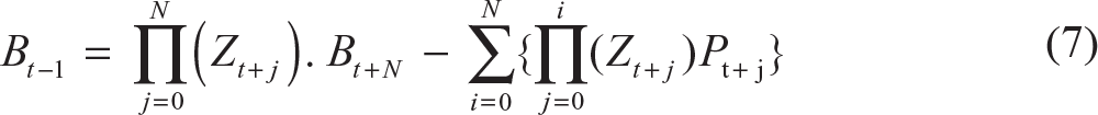
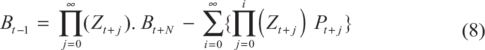
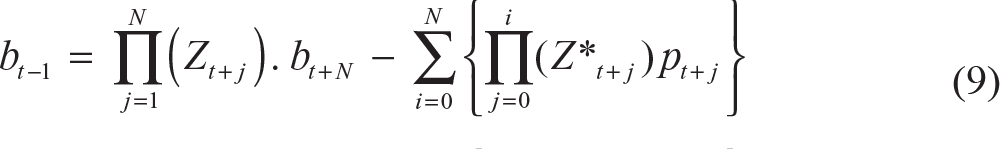
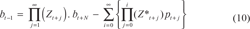
The Z in Equations (7) and (8) and Z* in Equations (9) and (10), respectively represent (1 + r) and {(1 + g)/(1 + r)}. The terminal value of debt, that is, B_t+N and b _t+N , indicates stock of debt and ratio of debt to GDP at t + N period. The requirement of sustainability of public debt is that the sum of present discounted value (PDV) of future PS should be at least equal to the present period stock of debt. In other words, the left hand side (LHS) of Equations (7) and (8), and Equations (9) and (10) should be at least equal to the right hand side (RHS) of the respective equations. Following this, we have:

B_{t - 1} = - \sum_{i = 0}^{N} {\prod_{j = 0}^{i} (Z_{t + j}) P_{t + j}}

(11)

B_{t - 1} = - \sum_{i = 0}^{\infty} {\prod_{j = 0}^{i} (Z_{t + j}) P_{t + j}}

(12)

B_{t - 1} = - \sum_{i = 0}^{N} {\prod_{j = 0}^{i} (Z *_{t + j}) p_{t + j}}

(13)

B_{t - 1} = - \sum_{i = 0}^{\infty} {\prod_{j = 0}^{i} (Z *_{t + j}) p_{t + j}}

(14)

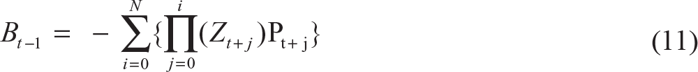
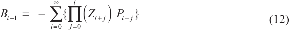
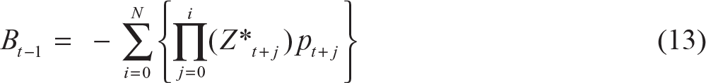
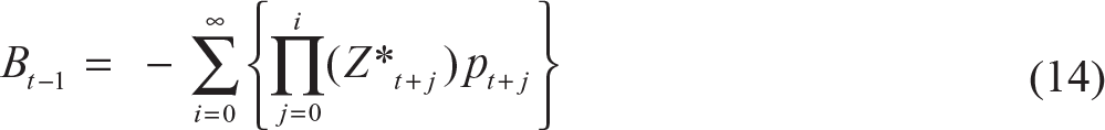
The minus sign of the primary deficit in Equations (11), (12), (13) and (14) indicates PS. This implies that the first term of RHS of Equations (7), (8), (9) and (10) should be negative or zero. The essential meaning of this condition is that the PDV of net public debt (difference between the present stock of debt and sum of PDV of future PSs) is zero at the terminal point due to the assumption of dynamic efficiency. Following this we have:

\prod_{j = 0}^{N} (Z_{t + j}) . D_{t + N} = D_{T} \leq 0

(15)

\prod_{j = 0}^{\infty} (Z_{t + j}) . D_{t + N} = 0

(16)

\prod_{j = 0}^{N} (Z *_{t + j}) . d_{t + N} = d_{T} \leq 0

(17)

\prod_{j = 0}^{\infty} (Z *_{t + j}) . d_{t + N} = 0

(18)

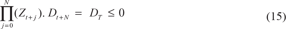
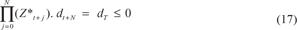
Two different types of terminal conditions are present in Equations (15), (16), (17) and (18). Super solvency is measured by less than zero while exact solvency is understood as equal to zero. Satisfaction of aforementioned conditions are required by current and future fiscal policy behaviour for sustainability of fiscal policy.

Empirical Framework for Solvency Approach

There are some practical difficulties in operationalisation of the solvency approach as it is difficult to know with accuracy about future values of debt and PSs. As a consequence, researchers rely on historically given past data on important fiscal variables like primary deficit or surplus, government revenues and expenditures or public debt (Bohn, 1998; Hamilton & Flavin, 1986; Wilcox, 1989). Mostly, researchers have applied time series econometric applications like unit root test and co-integration or vector auto regression in addressing the question of fiscal sustainability. However, the underlying assumption is the continuation of historically given trends and patterns. Because the empirical nature of the solvency approach depends on historically given information on relevant variables, it is called a backward-looking approach to fiscal sustainability (Pradhan, 2015b). Though the essence of fiscal sustainability assessment is forward-looking, for all practical purposes, the empirical framework for the solvency approach becomes backward-looking.

There are some limitations of the approach. Maintenance of IBC is highly technical, not easy to interpret and makes highly restrictive assumptions such as that of dynamic efficiency. At all points of time, it may not be possible to honour IBC, and non-satisfaction of IBC for some years does not mean that the government is facing an immediate threat of insolvency. It also assumes selection of appropriate discount rates and the terminal point at which the PDV of debt be zero is very difficult to attain. That is why Buiter and Patel (1992) mentioned that honouring IBC is a weak solvency criterion. To overcome it, they suggested focusing on strong and practical aspects that determine solvency and fiscal stability, the debt-to-GDP ratio or debt-to-revenues ratio and ratio of different debt servicing to either revenues or export or GDP. In this context, maintaining low debt-to-GDP ratio or other indicators as set by a country’s feasible fiscal policy framework are the best indicators of fiscal sustainability. The ultimate requirement of sustainability asks that debt-to-GDP ratio or other indicators like interest payment to revenue or GDP ratio should not grow explosively and unboundedly.

The fiscal reaction function (FRF) test of Bohn (1998) is also widely used to examine fiscal sustainability. The FRF tests whether PS responds positively with change in public debt. It also follows the co-integration of primary surplus-to-GDP ratio and public debt-to-GDP ratio. However, Ghosh, Kim, Mendoza, Ostry, and Quereshi (2013) argued that a positive relationship between PS and public debt though necessary may not be a sufficient condition if the initial debt stock is too high or if the PS is not large enough to account for the exploding interest rate growth differential or if the adverse reaction of the financial market is accounted for. Ghosh et al. (2013) call Bohn’s condition a weak sustainability condition and alternatively they developed a new framework called fiscal space in assessing debt sustainability. Fiscal space is defined as the distance between the current debt level to the debt limit beyond which debt sustainability is in doubt.

Fiscal Projection and Fiscal Gap Approach

So far whatever we have discussed above is mainly based on historically given time series data and that is why the approaches adopted thus far are called backward-looking approaches. Nothing is said about the future evolution of relevant fiscal variables for studying the sustainability aspect. Considering this limitation of backward-looking approaches, literature has developed projection methodology of several fiscal parameters to judge the LT sustainability of fiscal policy based on theoretical frameworks developed earlier. To highlight the importance of fiscal projection it is important to note that such projections provide invaluable signposts to help current government to respond to known fiscal pressure and risk in gradual manner…help future government to avoid abrupt policy change’ (Organisation for Economic Cooperation and Development [OECD], 2014). Fiscal projection to know future dynamics of fiscal policy is called a forward-looking approach. To know the LT sustainability based on comprehensive fiscal projections, it is important to know the concept of fiscal gap (FG) analysis (Auerbach, 1994). FG is defined as the immediate and permanent increase in PS to attain a pre-determined or current level of debt-to-GDP ratio in future. FG conveys through a single number the magnitude of PS necessary to avoid unsustainable increase in debt-to-GDP ratio or to maintain the IBC requirement. FG is also calculated both in finite and infinite time horizons to assess sustainability. Technically, FG can be developed following the Fiscal Sustainability Report of Government of Canada (2012).

Let us assume that the projected primary surplus is $\bar{P S}$ . If the current debt level is unlikely to equal PDV of all future PS, FG is then the difference between current debt level and projected primary balances, that is, $\bar{P S}$ . If FG is denoted as Δ, a constant proportion of projected GDP (denoted as Y), to attain equality between debt level and PDV of primary surpluses, then:

Δ = \frac{B_{t - 1} - \prod_{j = 1}^{N} (Z_{t + j}) B_{t + j} - \sum_{i = 1}^{N} {\prod_{j = 1}^{i} (Z_{t + j}) \bar{P S_{t + j}}}}{\sum_{i = 1}^{N} \prod_{j = 1}^{i} (Z_{t + 1}) \bar{Y_{t + j}}}

(19)

FG calculation for absolute level of debt for finite and infinite horizon

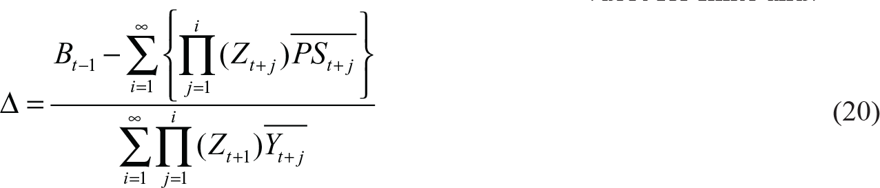
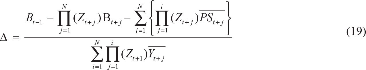
Δ = \frac{B_{t - 1} - \sum_{i = 1}^{\infty} {\prod_{j = 1}^{i} (Z_{t + j}) \bar{P S_{t + j}}}}{\sum_{i = 1}^{\infty} \prod_{j = 1}^{i} (Z_{t + 1}) \bar{Y_{t + j}}}

(20)

The FG calculation in terms of debt-to-GDP ratio for a finite period assumes that at the end of the projection, the hypothetical debt-to-GDP ratio is d^*, then we have:

Δ = \frac{b_{t - 1} - \prod_{j = 1}^{N} (Z_{t + j}) d *_{t + j} - \sum_{i = 1}^{N} {\prod_{j = 1}^{i} (Z *_{t + j}) \bar{p s_{t + j}}}}{\sum_{i = 1}^{N} \prod_{j = 1}^{i} (Z_{t + 1}) \bar{Y_{t + j}}}

(21)

FG calculation for debt to GDP ratio for finite and infinite horizon

Δ = \frac{b_{t - 1} - \sum_{i = 1}^{\infty} {\prod_{j = 1}^{i} (Z_{t + j}) \bar{p s_{t + j}}}}{\sum_{i = 1}^{\infty} \prod_{j = 1}^{i} (Z *_{t + 1}) \bar{Y_{t + j}}}

(22)

The interpretation of Z, Z^*, Bt, Bt _{+ 1}, bt and b_t+1 are the same as in section ‘Solvency Approach’. The denominator in each equation is the PDV of income of the country (i.e., GDP).

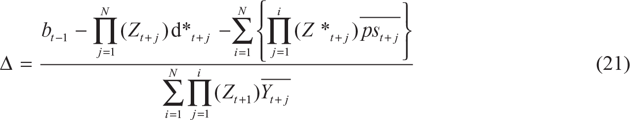
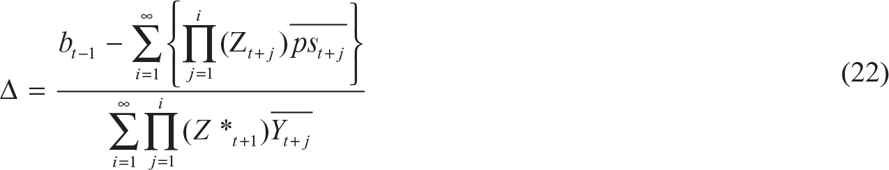
Empirical Framework for Fiscal Projection Approach

To assess fiscal sustainability through the fiscal projection framework, one needs to compute the FG or sustainability gap (SG), that is, Δ. However, Δ depends on discounted value of public debt, projected value of primary surplus, GDP, interest rate on borrowing and GDP growth rates. Due to difficulty in getting accurate forecasted values of the above variables, FG has little empirical application. Moreover, due to the cumbersome formula for computing FG, its application is very limited in empirical research. To overcome this problem, the forward-looking approach assesses fiscal sustainability in terms of comparing projected debt-to-GDP ratio to any benchmark or threshold debt-to-GDP ratio. The forward-looking approach is also useful as it can assess the fiscal sustainability of programme-specific public-funded programmes like the proposed Universal Health Coverage (UHC), Universal Basic Income (UBI) or Universal Social Pension Scheme (USPS) in the Indian context which would likely to exert significant fiscal pressure on government in future.

Forward-looking Approach

The forward-looking approach largely relies on comprehensive projections of important fiscal and macro variables. A mechanical projection based on past information on fiscal macro variables would be of very little importance as future changes in demographics, productivity, bond yield, growth rate of economy and introduction of publicly funded expected programme and reforms are not incorporated. That is why it is extremely important to develop a suitable projection framework which overcomes the shortcomings of the backward-looking approach. The forward-looking approach is important in assessing fiscal sustainability of government-funded programme’s specific expenditures in terms of projected debt-to-GDP ratio. If the projected debt-to-GDP ratio does not increase rapidly or does not cross certain threshold levels, the programme is said to be fiscally sustainable.

Based on a study by Pradhan (2015b), a simple framework for forward-looking approach to accommodate any publicly funded programme in terms of projected debt to GDP can be developed as following.

Taking cues from the framework developed in section ‘Solvency Approach’, one can rewrite Equation (6) as follows:

b_{t} = {(1 + r_{t}) / (1 + g_{t})} b_{t}_{- 1} + p d_{t}

(23)

To obtain the future path of b_t in Equation (23), the projection exercise should yield credible information r_t, g_t and pd_t. Evolution of r_t, g_t and pd_t would shape the dynamics of debt-to-GDP ratio in future. The future fiscal-financial implications of any expected government programme or reforms in existing programmes can be evaluated by assessing the additional expenditures over and above the existing expenditure. Fiscal sustainability of additional expenditures would largely shape the sustainability of the expected publicly funded programmes. Fiscal sustainability of the additional expenditures is assessed in terms of its impact on future path of debt-to-GDP ratio, keeping other things unchanged. To incorporate this additional spending over and above the existing government expenditure, we need to modify Equation (23). The modified version is given as:

b_{t} = {(1 + r_{t}) / (1 + g_{t})} b_{t}_{- 1} + {p d_{t} + x_{t}}

(24)

The term x_t in Equation (24) is the required additional government spending-to-GDP ratio over and above the existing spending on the programme. Therefore, the sum of pd_t and x_t {i.e., pd_t + x_t} can be called modified or new primary deficit ratio on account of a new programme. In the Indian context, due to persisting primary deficit, financing of additional expenditures, that is, x_t, would be debt financed. Thus, it is highly important to project the value of x_t after incorporating detailed provisions of a new programme in evaluating its fiscal impacts.

Empirical Framework for Forward-looking Approach

The forward-looking approach mainly assesses the fiscal implication of proposed programme-specific expenditure by the government. The question that arises here is whether or not the additional expenditure, on account of the proposed programme, over and above the existing fiscal and macroeconomic structure would be fiscally sustainable in terms of the future time path of debt-to-GDP ratio, and comparing it with some threshold level. Financial burden depends upon the provisions of the programme also. Therefore, studying the detailed provisions and computing the associated financial burden is essential in determining the fiscal sustainability of the programme. Then one can provide the baseline projection of debt to GDP from a medium- to long-term planning horizon. Sensitivity analysis is essential to any forward-looking projection because the baseline result is arrived at after assuming a particular set of values of the parameters of the projection framework. In the present context, fiscal sustainability results are highly sensitive to values of the growth rate of the economy, bond yield and baseline primary deficit. For sensitivity analysis, different values of interest rate, primary deficit and productivity growth rate are assumed to provide alternative scenarios.

Many a times, it may happen that the additional financial burden of the proposed programme is not fiscally sustainable. In this scenario, the relevant question is how to avoid fiscal unsustainability of the programme. One may note from Equation (24) that the future dynamics of debt-to-GDP ratio, apart from x_t and pd_t, depends on GDP growth rate (g) and interest rate of government borrowing (r). Therefore, to restore fiscal sustainability, the required adjustment should take place with the parameter of the model, that is, r, g, or pd.

Inter-generational Equity

The approaches discussed above do not pay any explicit attention towards generational equity, which can add another dimension to LT fiscal sustainability analysis. The previously outlined concepts and application of fiscal sustainability do not necessarily imply that the outcome will be also generationally fair (Kotlikoff, 1999). ‘As with the concept of long-term fiscal sustainability, there is no unique definition of what ‘inter-generationally fair’ means, as it can be defined from different perspectives’ (HM Treasury, 2008, p. 20). Generational equity can be defined when all generations pay the same amount of net transfer or the same share of their income to the government. It can also be defined on the basis of ability to pay the principle of different generations to the government, or that after net transfer, utility of all generations remain the same. It is generally argued that as a nation becomes richer due to productivity gains and technological innovation, future generations should pay a larger net transfer to the government than the present generations.

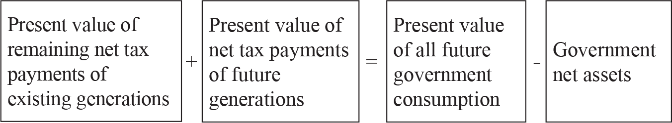
Assessment of generational equity is based on generational accounts (GA) and is defined as the present value of taxes paid net of transfer payments (i.e., net transfer to government) as the remaining lifetime across generations should be equal. Auerbach, Kotlikoff, and Leibfritz (1999) were the pioneers in developing the methodology of GA which is used for LT fiscal policy analysis and planning. According to them, the government’s IBC at each point of time requires that the subsequent net tax payments of the living current and the yet-to-be-born future generations be sufficient in present value terms to cover the present value of future government consumption expenditures, as well as pay off the government’s net indebtedness.

Equation (25) presents the aforementioned idea of GA in algebraic form:

\sum_{s = 0}^{D} N_{t, t - s} + \sum_{s = 1}^{\infty} N_{t, t + s} = \sum_{s = 1}^{\infty} G_{s} {(1 + r)}^{t - s} - W_{t}^{g}

(25)

The first summation of the LHS of Equation (25) is the present value of net tax (N_t) payments of the generation born at period t – s with maximum length of life being fixed at D, that is, the present value of the net tax payments of existing generations. The second summation of the LHS is the present value of net tax payments of infinitely lived future generations. The first summation of the RHS of Equation (25) is the present value of all future government consumption expenditures, while the second term of RHS is the value of net asset position. Equation (25) demonstrates that unless one knows the future time path of G_s (i.e., government purchases) and GAs of currently alive, one cannot determine the fiscal burden imposed on future generations. Therefore, to assess the generational stance of fiscal policy, assumptions and projections about future evolutions of fiscal and macroeconomic variables are essential. However, the underlying projection methodology of GA is similar to fiscal projections or the forward-looking approach to fiscal sustainability (Giammarioli, Nickel, Rother, & Vidal, 2007). In GA, all living generations are used to compute total revenue and total expenditures in net present value terms. In a similar fashion, FG or SGs are estimated, which are assumed to be borne by all future generations. But there are several limitations of GA. It is extremely data intensive as it needs information about different ‘cohort’ groups and distribution of all current payment streams between the government’s accounts and households.

Empirical Framework for Generational Equity

A GA software is used to assess whether government spending and tax programmes benefiting the current generation will produce an unfair tax obligation for future generations. GA is a tool in understanding the inter-temporal imbalance in public finance. In Equation (25), W_t ^g is the net asset (or liability) of the government and is known a priori. For a given interest rate, if the future path of government expenditure (i.e., G _s ) is known, the first term of RHS of Equation (25) is known. Thus the RHS of Equation (25) is the net PDV of government liabilities. How this burden is distributed among currently living members and yet-unborn members is to be decided for generational fairness. If current and future generations, after adjustment for productivity growth, pay equally to match the net discounted burden, the current fiscal policy is generationally fair and sustainable. The GA software computes this given the wide-ranging projections of population growth, productivity growth, interest rate and time path of government spending.

Ricardian Equivalence Approach

Taxes and public debt are two instruments of financing government expenditures. Current taxes are a burden on the present generation while deficit or public debt are taxes on future generations. Therefore, deficit or debt are implicit taxes and substitution of taxes by public debt is nothing but rearrangement of timing of taxes. Public debt is the postponement of taxes and involves higher future tax burdens. Both taxes and debt thus affect welfare of current as well as future generations. The core substance of Ricardian equivalence is the generational welfare neutrality of these two fiscal instruments. If taxes and debt financing have a differential or non-neutral impact on current and future generations, fiscal policy is uneven in a generational welfare context and hence is unsustainable. Therefore, the understanding of the Ricardian equivalence approach to fiscal sustainability is more or less the same as the generational accounting approach. The RET is based on several assumptions. The main assumptions are (a) perfectly foresighted and altruistic economic agents, (b) perfect capital market; that is, lending and borrowing rates for different agents like government and private sectors are the same. Also the market interest rate and individual agent’s subjective discount rate between present and future consumption decisions are equal, (c) taxes are non-distortionary. In other words, government imposes only lump sum taxes on individuals and (d) individuals are rational and take any economic decision through optimisation of their objective function subject to budget constraints. Rational individuals also perfectly foresee the future path of government spending and can compute the PDV of future tax liabilities. In other words, households under the assumptions of RET are like neoclassical agents whose computational skill overcomes all kinds of un-systemic errors. Under these assumptions, RET states that deficit financing in place of taxes does not have significant impact on consumption, savings, investment and economic growth. Future taxes are fully perceived and discounted by the likes of neoclassical individuals while optimising their decisions. As a consequence, rational households save more and bequeath their wealth to future generations. In other words, no burden of public debt gets shifted to the future and hence the welfare neutrality of taxes cut deficit financing.

RET to fiscal sustainability is analysed with respect to generational welfare neutrality by the choice of financing instrument (i.e., tax and deficit) of government expenditure. According to the Ricardian approach, fiscal policy is sustainable if the choice of financing instrument of government expenditure does not affect generational welfare neutrality adversely. Using the seminal paper of Barro (1974), one can present an analytical framework of RET to fiscal sustainability in the following manner.

For sake of simplicity, we consider a two-period model, that is, t and t + 1 or t – 1 and t. The model is about an optimisation problem of a representative household with all relevant assumptions of RET. The model incorporates government and its fiscal policy. We denote household’s consumption and income, government expenditures and taxes as As and Is, Gs and Ts, respectively. Real interest rate or discount rate in the economy is denoted as r. Given this information one can write a two-period IBC of the household as follows:

A_{t} + A_{t}_{+ 1} / 1 + r = I_{t} + I_{t}_{+ 1} / 1 + r

(26)

There is no government in Equation (26). Incorporating government with balanced budget (i.e., T = G in both the periods) we can have Equation (27).

A_{t} + A_{t}_{+ 1} / 1 + r = (I_{t} - T) + (I_{t}_{+ 1} - T) / 1 + r

(27)

As balanced budget is an exception rather than reality for most countries including India, we bring the issue of deficit budget without changing government expenditures. That means, we reduce taxes in period t and increase it in t₊₁. Let us consider that taxes in t is T₁ < T = G and the same in t₊₁ is T₂ > T = G. Incorporating these together we get Equation (28).

A_{t} + A_{t}_{+ 1} / 1 + r = (I_{t} - T_{1}) + (I_{t}_{+ 1} - T_{2}) / 1 + r

(28)

Equation (28) incorporates deficit budget at period t, that is, T₁ < T = G. The deficit amount is denoted as D_t and expressed as D_t = T – T₁. It is assumed that D_t will mature in t₊₁ and the maturity value is denoted as D_t+1 and expressed as D_{t+ 1} = (1 + r) D_t.

Therefore, one can modify Equation (28) and express it as Equation (29).

A_{t} + A_{t}_{+ 1} / 1 + r = (I_{t} - T_{1}) + (I_{t}_{+ 1} - T_{2}) / 1 + r + D_{t}_{+ 1} {= (1 + r) D_{t}}

(29)

Apart from households, we have government in the economy. Therefore, we need to express the budget constraint of the government also. Revenue earned in period t and t₊₁ are T₁ and T₂ and non-interest bearing expenditures are G_t and G_t+1, respectively. The government has to also pay the amount of the value of bond (D_t) and interest burden (r) in period t₊₁. Thus, the budget constraint of government is expressed in Equation (30).

T_{1} + T_{2} / 1 + r = G_{t} + G_{t}_{+ 1} / 1 + r + D_{t}_{+ 1} {= (1 + r) D_{t}}

(30)

Equation (30) represents the government’s IBC. This is also known as solvency constraint (GSC), which is essential to persuade the private sector to lend to the government by purchasing government bonds. The objective of the household is to maximise its inter-temporal utility function, which depends upon consumption level at period t and t₊₁’, that is, A _t and A _t+1 subject to budget constraints represented by Equation (29).

One should keep in mind that the household not only considers budget constraints of its own, but also the budget constraints of the government. In general, under the classical optimisation technique, individuals optimise with respect to their own budget constraints. However, in RET, a household in addition to its own budget constraints also takes into account the budget constraints of the government. According to Kormendi (1983), RET works under the framework of a consolidated approach to model consumption function where both the private sector and the government do optimise with respect to all other budget constraints. This is strikingly different from the standard neoclassical approach of consumption modelling where optimisation of the private sector takes place in isolation of the government’s budget constraint (Kormendi, 1983). Thus, following Kormendi (1983), the resultant optimisation problem of the private sector can be expressed as follows:

Maximise U = U (A_t, A_t+1),

Subject to A_t + A_t+1/1 + r = (I_t – T₁) + (I_t+1 – T₂)/1 + r + D_t+1 {= (1 + r) D_t} and T₁ + T₂/1 + r = G_t + G_t + 1/1 + r + D_t + 1{= (1 + r) D_t}

The above optimisation problem incorporates the true spirit of the consolidated approach to consumption function modelling. Already it is stated that budget deficit is future taxes. Future generations would bear undue burden of these future taxes if they are not discounted by households at present. Such undue future tax burdens would reduce the welfare of future generations and would breach the objective of inter-generational equity. That is why a consolidated approach to model the consumption function is required to uphold the spirit of Ricardian equivalence for inter-generational equity. And any violation of inter-generational equity or generational welfare neutrality amounts to unsustainable fiscal policy.

Therefore, under the assumptions of RET, the forward-looking household would substitute Equation (30) into Equation (29) to get Equation (31).

A_{t} + A_{t}_{+ 1} / 1 + r = {I_{t} + I_{t}_{+ 1} / 1 + r} - {G t + G_{t}_{+ 1} / 1 + r}

(31)

Equation (31) is the consolidated and effective budget constraint of the private sector and is independent of taxes (Ts) and deficit (D). The true tax burden is the government expenditure, not current taxes, because whatever is spent by the government must be matched by the tax revenue at present and in future. Thus, the optimisation of the household subject to Equation (31) would provide an optimal solution of A_t and A_t+1, which would be independent of taxes and deficits but dependent on income (I) and government expenditures (G). This is what the core RET conveys.

However, empirical validation of RET for generational welfare neutrality of fiscal policy instruments like taxes, deficits, government expenditures or public debt in terms of their impact on important macro variables like consumption, savings, investment and economic growth requires proper econometric modelling, construction of variables, collection of data, appropriate techniques of estimation and diagnostic checks. The Ricardian approach to fiscal sustainability requires that the substitution of tax by deficit financing should not make the current generation well off by augmenting A_t and shifting the burden of repaying debt to future generations and hence reducing A_t+1. Equation (30), being GSC, guarantees that both generations cannot be made be better simultaneously with choice of tax cut deficit financing under the assumption of dynamic efficiency. However, if the current generation behaves as per the predictions of RET, no generation would be better off. This in turn ensures fiscal sustainability in terms of neutrality of generational welfare. That is why the empirical literature has focused on assessing the consumption modelling of the current generation with reference to fiscal policy instruments in examining the empirical validity of RET and fiscal sustainability.

Empirical Framework for RET to Fiscal Sustainability

The empirical framework for RET to fiscal sustainability has been developed by the test of aggregate consumption function, investment function, Euler equation,⁶ economic growth, twin deficits hypothesis (i.e., budget deficit and current account deficit), etc. How these tests are conducted with specification of equations, parameter restrictions, estimation problems and interpretation of results are described in detail by Seater (1993).

Balance Sheet Approach

The BSA addresses the shortcomings of traditional debt sustainability analysis (DSA) to fiscal sustainability by considering the disaggregated analysis of existing fiscal and external structures of the economy to account for risk and vulnerability of financing deficit or rollover of debt. Traditional DSA focuses on the aggregate measures of debt and neglects the disaggregated measures of fiscal or external sectors. The origin of BSA can be traced to the re-genesis and resolution of episodes of various types of macroeconomic crises. For instance, the financial and currency crises of East Asian countries in 1997–1998, and the fiscal and external debt crises of Latin American countries during the mid-1990s to early 2000s. According to an International Monetary Fund (IMF) study (2004), BSA is an analytical framework to identify the sources of vulnerabilities and imbalances in different macroeconomic sectors of a country. Every macro sector may be represented by balance of stock (like assets and liabilities) and flow side (income/revenue and expenditure) match or mismatch with other sectors. By doing so, BSA assesses the risk of financeability or repayment obligations and financing needs of interlinked macro sectors like fiscal and external sectors and their possible transmission risk to cause a crisis. Financeability risk implies how easily a country or a government can finance its funding needs to avoid any ST payment or repayment obligation crisis.

Generally, in a developing country context, persistent fiscal imbalance causes rapid deterioration of external sector indicators and vice versa due to their close link through macroeconomic identity. BSA is actually the perception of financial markets about the risk involved in financing a country’s external financing needs or financing the budgetary deficit of the government. This is because borrowing from the financial market exposes the balance sheet weakness or vulnerability of the entity concerned. For instance, in the Indian context, the growing reliance on market borrowing due to the cessation of monetised deficit since 1997–1998 and rule-based fiscal policy management (like the FRBM Act, 2003) require scrutiny and analysis of government’s balance sheet risks by the creditors in assessing the creditworthiness of government to finance deficit (Pradhan, 2014).

In brief, we can discuss the link between balance sheet vulnerability and fiscal sustainability. Creditors’ assessment about soundness of government finance, irrational behaviour of investors or speculation about government’s ability or the capacity to absorb exogenous negative shocks like banking crisis or other contingent liabilities are important factors to determine fiscal vulnerability. Other factors influencing fiscal vulnerability are how the government’s borrowing programme affects savings—investment or current account balance, the international financial market environment, government default history or assessment of government finance by several credit rating agencies. A negative sign of fiscal stability initially reflects investors’ unwillingness to subscribe to government bonds leading to collapse of bond price or spike in bond yield to unsustainable levels triggering a sovereign debt crisis. Sometimes even if government finance is in bad shape with high level of debt and deficits persisting for a long time, it might not invoke a debt crisis if other macro variables like high level of savings, investments, growth and comfortable forex reserves are maintained (Hausman & Purfield, 2004).

BSA, which considers numerous fiscal, external and other important macroeconomic indicators, may not convey a uniform or unanimous conclusion in identifying balance sheet vulnerability of the fiscal or external sectors. Moreover, the unit of measurement of all indicators may not be the same which would create a problem for aggregation. To overcome these limitations, the IMF study (2011) developed a composite vulnerability index (CVI) covering all indicators in providing a uniform call on the issue of financeability risk.

The framework for constructing CVI is not difficult to understand. In general, transformation of the variables or indicators concerned to the respective standard normal variable would make them a unit-free number. This has an advantage in aggregation, which is not possible if indicators are in differential units. That is why, to construct the CVI, each indicator, let us say Xⁱ_t, can be transformed into a standardised Zⁱ_t score, where Zⁱ_t is a standard normal variate and defined as (Xⁱ_t – μ)/σ. The μ and σ are the usual notations used for mean and standard deviation (SD) of the concerned ith indicator over time or space as the case may be. The value of Z score of each indicator separately or combined has important meanings. For example, if Z score is equal to zero, it implies that the concerned value is close to the average of the group or concerned sector. On the other hand, higher negative value implies better performance while higher positive value indicates worse performance because we are measuring the vulnerability of an indicator. In order to generate the index for each category, one can transform the Z scores into a cumulative normal probability distribution with specified value of mean without changing the value of SDs. The specified value of mean depends upon the scale of measurement of vulnerability. For example, if one measures a vulnerability index on a scale of zero (0) to ten (10), then mean will be 5. That means the simple Z score, which is nothing but the value of a standard normal variate, is now transformed into an index with a specified scale of measuring vulnerability. In this example, the value of index exceeding 5 towards 10 implies a higher degree of financeability risk. On the other hand, an index value below 5 implies a lesser or absence of financeability risk.

Early Warning System (EWS)

One of the disadvantages of the above-mentioned approaches to fiscal sustainability is that they do not incorporate uncertainty while assessing it. The EWS takes into account the economic uncertainty underlying the dynamics of fiscal policy, public debt and other macroeconomic factors. It incorporates a comprehensive measure of the responsiveness of fiscal policies to economic shocks (van Ewijk et al., 2013). The European Commission, the IMF and the OECD often use EWS results for signalling the possibility of a fiscal crisis and subsequent surveillance measures (Koester & Nickel, 2014). The objective of EWS is to avoid build-up of huge macroeconomic, fiscal and financial imbalances in preventing the onset of any crisis (European Central Bank [ECB], 2014). The effectiveness of EWS depends on reliable and timely identification and assessment of risk indicators and conveying the same to policymakers in advance.

The assessment of EWS depends on a large number of fiscal and non-fiscal variables. These indicators together form the basis of signalling. The signalling mechanism of EWS works through four distinct steps (ECB, 2014). The first step is to identify episodes of fiscal stress based on past incidents. The second is to identify ‘potential or leading indicators’ for fiscal stress and defining a ‘signalling window’. The signalling window determines how far in advance EWS can signal fiscal stress. It may be six months or one year or more than one year. If it is one year, signalling sent by an indicator(s) can be expected to cause a fiscal crisis in the next one year. The third step involves determining a ‘critical threshold’ for each of the leading indicators on the basis of historical data of leading indicators and past episodes of fiscal stress. The fourth and final step is to aggregate all indicators into a CVI for signalling fiscal stress and policy surveillance.

Summary and Conclusion

The article has provided a comprehensive review of the available literature on fiscal sustainability adopted in different contexts and supplemented it with adequate technical notes and explanations which are not provided or explicit in literature. Each approach has theoretical and empirical applicability and implications as well as limitations. Theoretical superiority of one approach over the other does not imply that it is empirically appealing and vice versa. In this respect, it is quite difficult to establish the superiority of one approach over the others. For instance, the solvency approach is a theoretically superior concept compared to Domar’s stability, but its empirical application is cumbersome. Similarly, the forward-looking approach is undoubtedly better in judging a country’s fiscal vulnerability, but its results and implications suffer from a high degree of sensitivity to the assumptions about the future values of the variables and low degree of precision about the forecast results and possible endogenous problems among the variables concerned.

Considering various aspects of different approaches to FS, one could focus on the EWS and the BSA for ST vulnerability, since they are theoretically less demanding, empirically simple and more appealing for practical implications. That is why credit rating and other multilateral agencies like the IMF have adopted these approaches in the recent past. For LT assessment of FS, the inter-generational equity and Ricardian Equivalence approach would be best since generational equity is a LT normative requirement.

Acknowledgements

The article is based on the author’s PhD thesis from the University of Mysore through the Institute for Social and Economic Change (ISEC), Bangalore, under the supervision of Professor M.R. Narayana. The author acknowledges valuable comments and suggestions from the anonymous referees, which have been instrumental in revising the article. However, usual disclaimers apply.

Declaration of Conflicting Interests

The author declared no potential conflicts of interest with respect to the research, authorship and/or publication of this article.

Funding

The author received no financial support for the research, authorship and/or publication of this article.

Notes

Financeability implies how easily a government or a nation finances deficit, rolls over debt or external sector payment needs. It depends on the creditworthiness of the entities concerned and perception of financial market investors.

However, this exogenous relationship between n and r may not hold true, rather the relationship may be endogenous. Domar’s approach does not consider such a possibility.

However, indirect monetisation is still continuing due to the RBI’s intervention in secondary markets for government. securities, as part of overall monetary management by RBI.

Fiscal policy is sustainable but the government is technically insolvent as there is no liquidation of government debt through generating primary surpluses.

Dynamic efficiency is a concept used in economic growth literature. It is a type of Pareto optimum condition in which no generation (either current or future) can be made better off without reducing the welfare of the other generation. Samuelson (1958) and Diamond (1965) provided the condition of dynamic efficiency in their classic overlapping generation model by comparing GDP growth rate (say g) and marginal productivity of capital (say r; i.e. rate of return or rate of interest on borrowing). Samuelson defines equality between n and r as ‘biological optimum’ or ‘dynamic efficiency’. Biological optimum states that rate of return from capital should be at least equal to the biologically determined growth rate of population which determines the growth rate in neoclassical economics. Thus, the rate of return less than what biological optimum asks is a case of over-accumulation of capital and hence a case of dynamic inefficiency (i.e., r < g). When r < g, government is playing a Ponzi-game where it is borrowing ever-increasing amounts to service its debt and thus even if debt-to-GDP ratio declines due to r < g, such a policy is not desirable to any economy. A dynamic efficiency requirement prevents governments from the recourse of Ponzi finance.

Euler equation is the first order necessary condition of any constrained dynamic optimisation problem. As Ricardian equivalence is essentially a constrained dynamic optimisation problem, finding the optimal time path of consumption, the Euler equation test provides a very straight forward direct test for Ricardian equivalence. (Evans, 1988).

References

Auerbach

A. J.

(1994). The U.S. Fiscal Problem: Where we are, how we got here, and where we’re going. NBER Macroeconomic Manual , pp. 141–75.

Auerbach

A. J.

Kotlikoff

L. J.

Leibfritz

(Eds.). (1999). The methodology of generational accounting. In Generational accounting around the world (pp. 31–42). Chicago, IL: University of Chicago Press.

Barro

(1974). Are government bonds net wealth? Journal of Political Economy , 82(6), 1095–1117.

Barro

(1979). On determinants of government debt. Journal of Political Economy , 85(5), 940–971.

Bohn

(1998). The behavior of U. S. public debt and deficits. Quarterly Journal of Economics , 113(3), 949–963.

Buiter

Patel

U. R.

(1992). Debt, deficits and inflation: An application to the public finance of India. Journal of Public Economics , 47(2), 171–205.

Buiter

(2010). Fiscal rules in India: Are they effective? (NBER Working Paper No. 15934). Cambridge, MA: NBER.

Chakraborty

(2018). Monetary seigniorage in an emerging economy: Empirical evidences. International Journal of Economics and Finance , 10(5), 135–144.

Diamond

(1965). National debt in a neoclassical growth model. American Economic Review , 55(5), 1126–1150.

10.

Domar

E. D.

(1944). The burden of debt and national income. American Economic Review , 34(4), 798–827.

11.

European Central Bank (ECB). (2014 November). ECB Monthly Bulletin. Retrieved from https://www.ecb.europa.eu/pub/pdf/other/art2_mb201411_pp91-105.en.pdf?31cab98145fbf0f03737707972e7dfa5

12.

Evans

(1988). Are consumer Ricardian? Evidence for the United States. Journal of Political Economy , 96(5), 983–1004.

13.

Giammarioli

Nickel

Rother

Vidal

J. P.

(2007). Assessing fiscal soundness: theory and practice (Occasional Paper Series No. 56). Frankfurt: European Central Bank.

14.

Gosh

A. R.

Kim

J. I.

Mendoza

E. G.

Ostry

J. D.

Quereshi

M. S.

(2013). Fiscal fatigue, fiscal space and debt sustainability in advanced economies. Economic Journal , 123(566), F4–F30.

15.

Government of Canada. (2012). Fiscal Sustainability Report 2012 . Ottawa: Office of the Parliamentary Budget Officer. Retrieved from http://www.pbo-dpb.gc.ca/web/default/files/files/files/FSR_2012.pdf

16.

Hamilton

J. D.

Flavin

M. A.

(1986). On limitations of government borrowing: A framework for empirical testing. American Economic Review , 76(4), 808–819.

17.

Hausman

Purfield

(2004). The challenge of fiscal adjustment in a democracy: The case of India (IMF Working Paper No. 04/168). Washington, DC: International Monetary Fund (IMF).

18.

HM Treasury. (2008). Long-term public finance report: An analysis of fiscal sustainability. London: HM Treasury. Retrieved from http://news.bbc.co.uk/2/shared/bsp/hi/pdfs/12_03_08bud08_longterm_615.pdfhttps://www.bde.es/f/webbde/SES/Secciones/Publicaciones/PublicacionesSeriadas/DocumentosTrabajo/14/Fich/dt1418e.pdf

19.

IMF. (2004). Debt-related vulnerabilities and financial crises –an application of the balance sheet approach to emerging market countries . Washington, DC: Policy Development and Review Department, IMF. Retrieved from https://www.imf.org/external/np/pdr/bal/2004/eng/070104.pdf

20.

IMF. (2011). Measuring fiscal vulnerability and fiscal stress: A proposed set of indicators (IMF Working Paper No. WP/11/94), Washington, DC: Fiscal Affairs Department, IMF.

21.

Koester

G. B.

Nickel

(2014). Signalling fiscal stress in the Euro area: A country-specific early warning system. Retrieved from https://www.ecb.europa.eu/pub/pdf/scpwps/ecbwp1712.pdf?6095998a00653e420ec902850d50fe30

22.

Kormendi

R. C.

(1983). Government debt, government spending, and private sector behavior. American Economic Review , 73(5), 994–1010.

23.

Kotlikoff

L. J.

(1999). From deficit delusion to the fiscal balance rule: Looking for an economically meaningful way to assess fiscal policy. In Auerbach

Alan J.

Kotlikoff

Laurence J.

Leibfritz

Willi

(Eds.), Generational Accounting around the World . Chicago, IL: University of Chicago Press.

24.

Organisation for Economic Cooperation and Development [OECD]. (2014). Chile’s Supreme Audit Institution: Enhancing Strategic Agility and Public Trust. OECD Public Governance Reviews, OECD Publishing. Retrieved from https://www.oecd-ilibrary.org/docserver/9789264207561-en.pdf?expires=1556264210&id=id&accname=guest&checksum=E861B37BDD523C4883665CBE2C39B5D6

25.

Pradhan

(2014). Assessment of India’s fiscal and external sector vulnerability: A balance sheet approach (ISEC Working Paper No. 327). Bengaluru: ISEC.

26.

Pradhan

(2015a). Sustainability of India’s fiscal policy: An empirical analysis (Unpublished PhD Thesis). University of Mysore, Mysore.

27.

Pradhan

(2015b). Fiscal sustainability of India’s National Food Security Act 2013. MARGIN: The Journal of Applied Economic Research , 9(2), 33–156.

28.

Rajaraman

Bhide

Pattainaik

R. K.

(2005). A study of debt sustainability at state level in India . Mumbai: Reserve Bank of India.

29.

Roubini

Hemming

(2004). A balance sheet crisis in India? Paper presented at the IMF/NIPFP Conference on Fiscal Policy in India, New Delhi.

30.

Samuelson

P. A.

(1958). An exact consumption-loan model of interest with or without the social contrivance of money. Journal of Political Economy , 66(6), 467–482.

31.

Seater

J. J.

(1993). Ricardian equivalence. Journal of Economic Literature , 31(1), 142–190.

32.

Wilcox

D. W.

(1989). The sustainability of government deficits: Implications for the present value borrowing constraint. Journal of Money, Credit and Banking , 21(3), 291–306.

33.

van Ewijk

Lukkezen

Romagosa

H. R.

(2013). Early warning indicators for debt sustainability (CPB Policy Brief No. 08). The Hague: CPB Netherlands Bureau for Economic Policy Analysis.