
Abstract
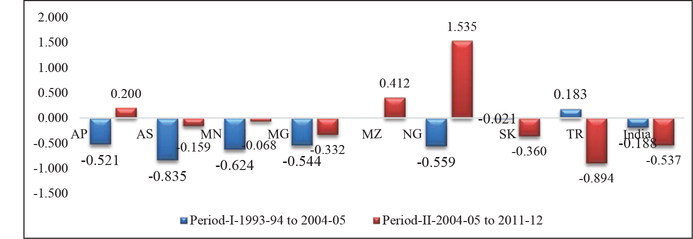
This study examines the changing structure of poverty and inequality for the northeastern states (NES) of India during the last two decades (1993–94 to 2011–12), by using the modified Kakwani poverty decomposition methodology, analysed by Bhanumurthy and Mitra (2004) based on the National Sample Survey Organisation’s (NSSO) consumer expenditure rounds. The estimates indicate that except for three states (Nagaland, Mizoram and Arunachal Pradesh), all other NES observed a decline in poverty, and Tripura recorded the highest decline in poverty in the second period (2004–05 to 2011–12). Further, an analysis of poverty–growth elasticity (PGE) reveals that only Arunachal Pradesh (0.200), Mizoram (0.412) and Nagaland (1.535) have greater PGE in the second period. A decomposition exercise of changing levels of poverty in terms of the three components—the growth effect, the inequality effect and the population shift effect—confirms that the positive impact of growth could not nullify the negative inequality impact on poverty.
The Indian economy has been undergoing spectacular change in its economic structure since the beginning of economic reform. A striking feature is that growth transformation has been accompanied by a moderation effect in the level of income with respect to poverty and inequality. The phenomenon of shrinking poverty accompanied by widening inequality in India has raised serious concerns in recent years for its implied ill fare and exclusion (Abraham, 2007; Chauhan et al. 2016; Mishra & Joe, 2010; Pal & Ghosh, 2007; Sen & Himanshu, 2004). Besides, such rising concerns on poverty and inequality across the globe have made the Millennium Development Goals and Sustainable Development Goals to emphasise the need to lessen the effect of poverty and inequality. Recent exploration by Ravallion (2020) offers a detailed account of the debates on this topic in the short history of ending poverty. Arndt et al. (2017) have discussed the importance of poverty–growth elasticity for understanding inclusiveness in the growth process. While analysing pro-poor growth in India, Datt and Ravallion (2011) observed that in the post-reform period there was an increase in inequality and that the urban–rural pattern of growth was responsible for the pace of poverty reduction. Deaton and Dreze (2002) postulated that regional differences widened in the last decade of the 20th century, with the southern and western regions performing better than the northern and eastern regions. At the same time, Datt and Ravallion (2002) highlighted that economic growth in the 1990s had not been experienced in states that would have a bearing on national poverty and therefore there was a need for analysing the sectoral and geographical composition of growth. The higher level of income inequality implied the income gains to the non-poor from distribution-neutral growth to be larger than the benefits to the poor (Ravallion, 2000). Rangarajan and Dev (2014) highlighted crucial points related to Rangarajan poverty estimates. This included new approaches for poverty line, public expenditure and poverty, use of calories, existence of high urban poverty, consumption differences (between National Accounts Statistics and National Sample Survey), and public spending. Further, they concluded that
policy should work towards not only to reduce the number of people below that line but also ensure that people, in general, enjoy a much higher standard of living. Numbers do indicate that the poverty ratio in India is coming down even though it may remain at a high level. Policymakers must continue to follow the two-fold strategy of letting the economy grow fast and attacking poverty directly through poverty alleviation programmes. (p. 19)
Subramanian’s (2011) study on poverty measurement analysed issues related to poverty estimates in India in terms of evaluation of methodology of poverty identification of 1993 and a critical assessment of the 2009 Tendulkar’s approach to the poverty line.
A common and persistent view has been that the benefits of high growth in the last two decades have had little impact on the poor in comparison to the benefits accruing to the non-poor. In other words, it may so happen that the positive effects of economic growth on the poor are likely to be counterbalanced by the negative effects of rising inequality appearing alongside economic growth. Here, it is essential to comprehend that the growth effect should outweigh the inequality effect in the context of rising inequality and decline in poverty. It essentially means that the extent of fall in incidence of poverty due to growth is higher than the rise in poverty due to an increase in inequality (Bhanumurthy & Mitra, 2004).
In this context, state-specific studies assume prime significance given the current policy emphasis towards achieving faster and inclusive growth across regions. Ahluwalia (2001) highlighted it as,
balanced regional development has always been one of the declared objectives of national policy in India and it is relevant to ask whether economic reforms have promoted this objective…since state-level performance shows considerable variation across states, with many states recording strong growth in the post reforms period, it is important to identify the reasons for their success in order to replicate it in other states. (p. 2)
Mohanty and Bhanumurthy (2018) emphasised that India manifests differential patterns with respect to regional growth. This finding proposes the requirement for diverse policy measurements for a different region of the states. Further, policy designs may also need to incorporate the adverse spillover effects of growth dynamics. A proper regional analysis of core socio-economic performances in terms of poverty, inequality, growth, employment and literacy is imperative for a proper understanding of these differences in development with state-level specificities. While there are numerous studies concerning national poverty and inequality, state-specific studies on the same aspect are limited (Chauhan et al. 2016; Rangarajan et al. 2007; Sen & Himanshu, 2004). Existing literature examining state-level economic growth, employment, poverty and inequality mostly covers only 17 major states of India; Assam is the only northeastern state (NES) in these studies (Bhaumik, 2007; Chadha & Sahu, 2004; De et al., 2017; Khan & Padhi, 2017; Konwar, 2015; Mahajan, 2009). Khan and Padhi (2017) examined the differential in poverty, inequality and relative deprivation among all NES of India during 2004–05 to 2011–12.
Although the existing research on understanding differential economic growth across regions exists, studies focused on NES, in particular, remain limited. Broadly, the NES are commonly referred to as “The Seven Sister States” and one brother state (Khan & Padhi, 2017), which belong to ‘Special Category Status’. Due to a lack of infrastructural development facilities with spatial location, the NES remain excluded from the rest of the country (Agnihotri, 2004). Other factors, such as predominance of agriculture sector, shortage of infrastructure and factories, political insurgency and violence and gross ignorance by the central government on special provisioning for these small states, make them lagged developmental states when compared with the rest of India (Sahu, 2012). Although the region is blessed with a unique culture and immense natural resource potential, their physical structure further isolates them from the rest of the country. This leads to development deprivation in the core economic sectors of a region (Cappellari & Jenkins, 2006). To promote growth and development in this region, a Department of Development of North Eastern Region was formed in 2001, which was three years later converted into a fully-fledged ministry—the Ministry of Development of North Eastern Region (Sahu, 2012). 1 However, it is disheartening that the NES have not received due attention in socio-economic studies including on poverty, inequality and employment. This is broadly due to the paucity of statistical and representative data sets (Khan & Padhi, 2017). Given the small sample collection in the NES, due to geographical constraints and limited statistical reliability of data, studies that comprehensively assess NES are limited (Khan & Padhi, 2017; Sahu, 2012; Srivastav & Dubey, 2003). Although topics related to poverty, inequality and employment have been debated in the last few decades and analysed for the major Indian states, only a few studies have discussed these aspects for the NES (Dikshit & Dikshit, 2014; NITI Aayog, 2015; Sahu, 2012; Sarma, 2015).
Further analysis with different forms of deprivation is important in order to highlight that consumption poverty in the NES is relatively different from that of the rest of the country when it comes to its implied extent of deprivation in other spheres of living. Here, questions that need to be analysed include the following: how does poverty in the NES relate to poverty in the rest of the country; how do other forms of deprivation, such as unavailability of proper infrastructural facilities, and unemployment relate to poverty in the NES; and what are the relative contributions of economic growth and redistribution to change in poverty in the NES. The primary question that has been addressed in this study is how the changes in poverty since the 1990s are linked to changes in economic growth, inequality and changes in population across NES. Such analysis enables us to perform a critical evaluation of the policies related to poverty alleviation and offers a comprehensive perspective of the reform process on poverty changes in the NES.
Our earlier study (Khan & Padhi, 2017) looked into different aspects of change in poverty, inequality and relative deprivation among NES by using the NSSO consumer expenditure surveys of 2004–05 and 2011–12. The present analysis reflects a broader perspective, where the changes in poverty and inequality among NES since liberalisation, in rural and urban areas, are looked in detail by using the poverty decomposition approach, with larger implications for policy analysis. Our study also contributes to the larger literature on the decomposition of poverty changes at subnational levels.
Data and Methodology
Data
For empirical analysis, the study made use of nationally representative large-scale consumer expenditure surveys undertaken by the NSSO. We explored the changes in poverty in the post-liberalisation era by decomposing changes in poverty over two time periods, namely, 1993–94 to 2004–05 and 2004–05 to 2011–12 for the rural and urban areas in India’s eight NES (Arunachal Pradesh, Assam, Manipur, Meghalaya, Mizoram, Nagaland, Tripura and Sikkim). We did not include the 1999–2000 and 2009–10 periods in our analysis because of certain limitations in the survey period (for details, see National Sample Survey Office, 2014, p. 1). The data were collected based on household characteristics and for different items of household consumption expenditure. To calculate the real monthly per capita consumption expenditure (MPCE) figures, the Consumer Price Index for Agricultural Labourers (CPI-AL) was used for rural areas, and Consumer Price Index for Industrial Workers (CPI-IW) was used for urban areas.
The methodologies for calculation of poverty in India are based on the recommendations of several working groups and expert committees as well as by the planning commission. These include a working group of the planning commission on poverty estimation (1962), Y. K. Alagh committee (1977), the expert group under the chairmanship of D. T. Lakdawala (1989), S. D. Tendulkar estimates (2005) and Rangarajan poverty estimates (2012; for details, see Rangarajan & Dev, 2014). Poverty estimation based on the Tendulkar committee recommendation is an improvement over the Lakdawala poverty methodology. The Tendulkar poverty methodology applied the officially measured urban poverty line of 2004–05 based on the Lakdawala committee methodology (Rangarajan & Dev, 2014). The Rangarajan poverty estimates opted for the Mixed Modified Reference Period (MMRP) consumption expenditure for estimation of poverty. While our analysis has followed from 1993–94 to 2011–12, the MMRP poverty estimation information is available from 2009–10 onwards (Rangarajan & Dev, 2014). Due to this, for comparison and estimations, we skip the Rangarajan poverty estimation approach; instead, in this study, we opt for the Tendulkar poverty estimates (see for details, Expert Group to Review the Methodology for Measurement of Poverty, 2014). Accordingly, the data sets were structured for empirical analysis as suggested by Bhanumurthy and Mitra (2004). 2 By doing this, we presume that the number of people and the per capita consumption expenditure within the class interval are proportionately related in this study. 3
Methodology: Technical Note
Poverty Decomposition Methodology
The influence of growth on poverty reduction has been explored in the literature (see, for example, Ahluwalia, 1978; Bhanumurthy & Mitra, 2004; Datt & Ravallion, 1992, 2002; Jain & Tendulkar, 1990; Mitra, 1992). While Ahluwalia discussed agricultural growth’s benefits trickling down to the poor, Jain and Tendulkar (1990) explored the strength of growth and redistribution in changes in headcount poverty during the 1980s. Kakwani and Subbarao (1990) and Jain and Tendulkar (1990) 4 initiated discussion, in the Indian context, on decomposition of the change in poverty into growth and distribution effects.
Subsequently, Datt and Ravallion (1992), Kakwani (2000), Mazumdar and Son (2002) and others developed various alternative decomposition methods of change in poverty. Kakwani and Subbarao (1990) studied the changes in poverty into mean and inequality effects, but this methodology has certain limitations, such as the decomposition containing the ‘residual term’ in it and decomposition being not exact (Bhanumurthy & Mitra, 2004). The relative contributions of economic growth and redistribution to changes in poverty were quantified by Datt and Ravallion (1992). The estimated results can infer whether the changes in welfare distribution have offset gains from economic growth in reducing poverty. However, this ‘growth inequality decomposition’ method is ‘not symmetric’ and ‘sensitive’ to the base year (Bhanumurthy & Mitra, 2004).
Jain and Tendulkar’s (1990) methodology was criticised for using different periods in estimating mean and inequality effects. Subsequently, Kakwani (2000) proposed an improved method that addressed the lacunae in the earlier ones. Mazumdar and Son (2002) included the ‘population shift effect’ in the decomposition exercise, in addition to the growth and inequality effects analysed in earlier studies. They highlighted that the changes in the poverty index can be decomposed into three effects,
(i) any shift in population between the different segments with different degrees of poverty; (ii) the growth in income in each of the segments; and (iii) the change in the distribution of income, particularly at the lower end where the poor households are located. (p. 7)
Bhanumurthy and Mitra (2004) also used the Mazumdar and Son (2002) methodology to understand the changes in poverty in relation to changes in inequality and population shift effect for India. This study, by using various NSSO consumption survey rounds, found that the growth effect was pronounced over the inequality effect and the population shift effect in both periods. The growth effect shifted up in the reform period, which helped to reduce poverty, and the inequality effect fell during this period. Using the Bhanumurthy and Mitra (2004) methodology, Panda and Padhi (2020) analysed poverty decomposition for Odisha, and found that growth effect has higher share than inequality effect and population shift effect on poverty reduction. In the present article, the analysis of the modified Kakwani poverty decomposition methodology has been directly derived from Bhanumurthy and Mitra (2004). However, in this decomposition methodology, the population shift effect is indirectly computed from the change in poverty, growth and inequality effects. Further, the changes in poverty are decomposed into growth effect or mean effect (keeping inequality same), inequality effect (keeping growth constant) and population effect particularly for the NES of India. While analysing the population shift effect, the percentages of the population living in rural and urban areas are taken into account. Accordingly, the population shift in the growth process has been measured in this study.
Let the changes in poverty in two-round period x and y be

where P is the poverty headcount ratio, Z is the poverty line,

where


So, the decomposition can be presented as
Besides the growth and inequality effects, Mazumdar and Son (2002) included the role of population shift in decomposition analysis. This can be explained by assuming that there are two subpopulation groups, I = 1 and 2, and the rate of change in the poverty index can be shown as presented by Bhanumurthy and Mitra (2004)
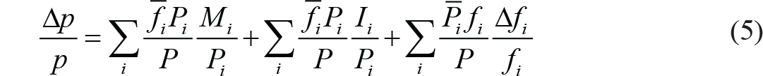
where the left side of equation (5) shows the proportion change in poverty, while the right side of equation (5) reveals growth effect, inequality effect and population growth effect. Further,

where
In this case, the subscript i represents rural and urban places.
Gini Coefficient
In this study, the Gini coefficient has been used to measure inequality in the distribution based on the MPCE measured through mixed reference period (as a proxy for income) data sets. The Gini coefficient
5
varies between 0 and 1 (Dutta, 2005; for a detailed understanding of the methodology, see also Chauhan et al., 2015; Haughton & Khandker, 2009), and it is described as follows:
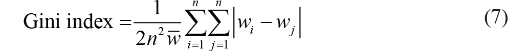
where n is the number of individuals in the sample; w is the arithmetic mean per capita consumer expenditure;
Poverty–Growth Elasticity
The impact of economic growth on poverty reduction is often calculated through the growth elasticity of poverty. The poverty–growth elasticity (PGE) is calculated based on the studies of Arndt et al. (2017) and Ram (2011). Using the growth in incidence of poverty (headcount poverty) and growth of gross state domestic product (GSDP; growth based on 2004–05 base year price) the PGE is calculated as
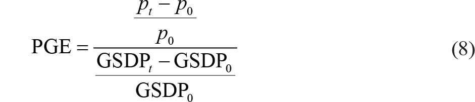
where
Results and Analysis
Economic Growth, Poverty and Inequality in Northeastern Region of India
The results of overall poverty, inequality and growth in GSDP for the last two decades for the eight NES and for India are reported in Table 1. The growth rate in GSDP is given as per the 2004–05 base year price (for 1993–94, 2004–05 and 2011–12) and the poverty (based on Tendulkar estimates) and inequality (Gini inequality) figures are shown as the only difference between poverty headcount and the Gini difference between periods I and II. 6 The results portray some interesting insights. The compound annual growth rate is shown in the GSDP figures at the 2004–05 base year price. The estimates reflect that, in both period I (1993–94 to 2004–05) and period II (2004–05 to 2011–12) all the NES reflect a differing pattern for changes in growth, poverty and inequality (Table 1).
Poverty, Inequality and Growth (GSDP) Dynamics
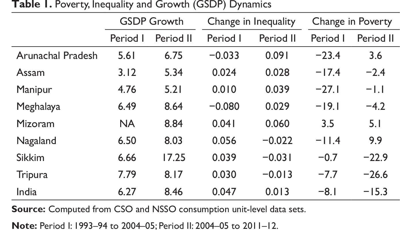
Most of the states exhibit declines in the level of headcount poverty in the post-liberalisation era. In the first period, the highest decline in poverty comes from Manipur (−27.1 percentage points), and the lowest decline in poverty is from Sikkim (−0.7 percentage points), while in the second period, the highest and lowest declines are from Tripura (−26.6 percentage points) and Manipur (−1.1 percentage points), respectively. Although at the national level there is a decrease in incidence of poverty, for the NES, in period I, only Mizoram (3.5 percentage points) and Tripura (7.7 percentage points) show an increase in poverty, while in period II, only three states—Arunachal Pradesh (3.6 percentage points), Mizoram (6 percentage points) and Nagaland (9.9 percentage points)—accounted an increase in poverty.
As for the level of inequality (expenditure as a proxy of income), except Arunachal Pradesh (−0.033 decline) and Meghalaya (−0.08 decline), all other states show a rising level of inequality for period I. In the second period, except for Nagaland, Sikkim and Tripura, all states reflect an increase in inequality. Arunachal Pradesh (0.091) shows a rise in the degree of inequality while Sikkim shows the sharpest fall in the level of inequality (0.031).
In period I, Tripura showed the highest level of GSDP growth (7.79%). In period II, it was Sikkim (17.3%), followed by Meghalaya (8.6%) and Mizoram (8.8%) standing above the all-India growth rate. The lowest growth rate in period II is seen in Manipur (5.2%). Out of all the NES, in period II, only Sikkim shows an improvement in the level of three core indicators (growth, poverty and inequality) as compared to other NES, while in period I, Arunachal Pradesh and Meghalaya show improvements in all three indicators.
Poverty–Growth Elasticity
We analysed the impact of economic growth on poverty through the growth elasticity of poverty for all the NES during the last two decades. The growth elasticity of poverty and inequality elasticity of poverty were calculated by using the formula given by Arndt et al. (2017). The PGE estimates show a different picture for all the NES. At the all-India level, the PGE was −0.19 in the first period and −0.54 in the second period. These PGE components are quite diverse among the NES (Figure 1). Out of all the NES, only Tripura during period I and Nagaland during period II show the highest PGE as compared to other states, while Assam during period I and Tripura during period II show the lowest PGE. The estimates also show that Manipur reflects a lower poverty elasticity due to the higher reference year poverty rate in the first period. The same analysis can be explored for the second period as well. The PGE results depict that in period II, out of all the NES, only Arunachal Pradesh (0.20), Mizoram (0.41) and Nagaland (1.54) showed positive growth elasticity figures, while all other NES showed a negative value—Tripura (−0.89), followed by Sikkim (−0.36) and Meghalaya (−0.33).
Changing Nature of Poverty and Inequality in the Rural and Urban Areas of NES
Despite the NES showing a diverse picture in terms of decline in poverty and inequality, the rural and urban sectors reflect different pictures during period I (1993–94 to 2004–05) and period II (2004–05 to 2011–12) (Figure 2). 7 Our analysis shows that all the NES show different levels of poverty and inequality change across sectors during the last two decades. Urban poverty is less than rural poverty for all the NES; Meghalaya, Mizoram, Sikkim and Tripura had less than 10% poor in 2011–12 especially in urban areas (see Table 2 for details).
Changes in Poverty and Inequality in Rural and Urban Areas of the Northeastern States of India
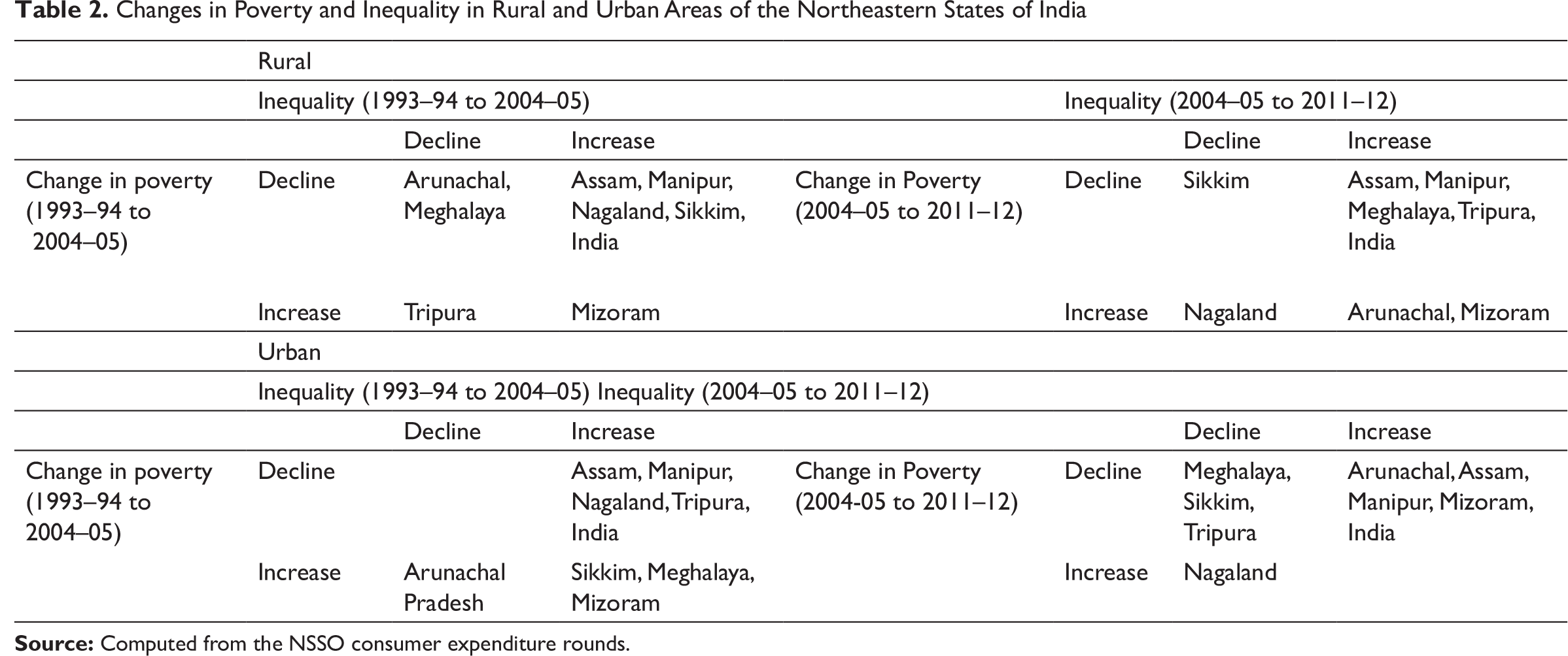
In rural areas, increase in both poverty and inequality is observed in Mizoram during period I, and Arunachal Pradesh and Mizoram during period II. During period II, both poverty and inequality declined only in Sikkim. In urban areas, in period II, Meghalaya, Sikkim and Tripura experienced a fall in both poverty and inequality, while in period I, no state exhibited declines in both poverty and inequality. Both in the rural and urban areas, during both of the periods, most of the NES exhibited an increase in the magnitude of inequality while decline in the levels of headcount poverty (Figure 2).

As per the Tendulkar poverty estimates, at the aggregate level, the level of household poverty in 2011–12 among NES was lowest in Sikkim (8.2%) and highest in Manipur (36.9%). Except for Arunachal Pradesh (3.6 percentage point increase), Mizoram (5.1 percentage point increase) and Nagaland (9.9 percentage point increase), all NES saw a decline in headcount poverty at the aggregate level in the second period. Sikkim (31.1%–8.2%) and Assam (34.4%–32%) showed a decline in poverty while Nagaland (9%–18.9%) showed a drastic increase in poverty.
Further, among NES, in rural areas, the headcount poverty estimate is lowest in Sikkim (9.9%) and highest in Arunachal Pradesh (38.9%), while in urban areas, poverty is lowest in Sikkim (3.7%) and highest in Manipur (32.6%). Similarly, in rural areas, Arunachal Pradesh (5.3 percentage points), Mizoram (12.4 percentage points), and Nagaland (9.9 percentage points), and in urban areas only Nagaland (12.2 percentage points) show an increase in the level of headcount poverty in period II. The pattern of changes in poverty in Arunachal Pradesh and Tripura is interesting. From 1993–94 to 2004–05, the decline in rural poverty was highest in Arunachal Pradesh, and there was a 10.2 percentage point increase in the level of household poverty in Tripura. In the recent period, however, Tripura shows a 28 percentage point decline in poverty in rural areas. The differential level of poverty and inequality changes is mostly due to better performance on socio-economic indicators and availability of infrastructure in these regions.
Poverty Decomposition Results
Table 3 presents the changes in poverty by growth effect (GE), inequality effect (IE) and population shift effect (PSE), as per the methodology, for eight NES in both rural and urban settings. The decomposition results show that poverty change over the last two decades has taken place with changes in various core macro- and micro-economic parameters. The decomposition result portrays interesting results for the NES in the post-liberalisation era. In a few states, poverty increases or decreases accounted for the increase or decrease in the growth, inequality and population shift effects.
Decomposition of Change in Poverty Between 1993–94 to 2004–05 and 2004–05 to 2011–12
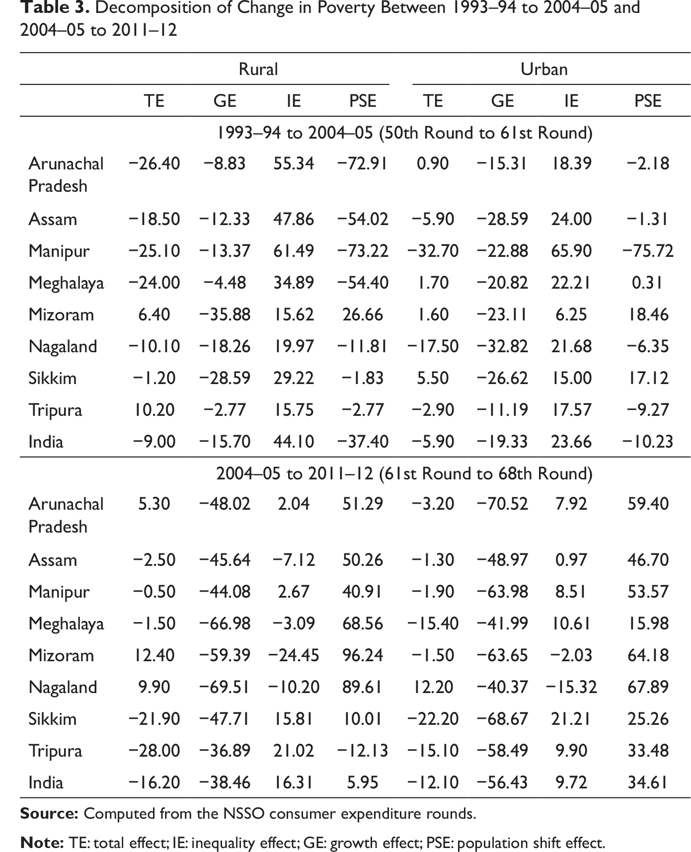
From Table 3, it can be noted that in period I, the inequality effect and PSE dominated over the growth mean effect in most of the rural areas of NES. Further, the growth/mean effect and PSE dominated over the inequality effect during the second period, which displays a fall in the estimated level of poverty in both the periods. Even in rural Mizoram and Tripura during period I, and Mizoram and Nagaland in Period II, the observed poverty ratio increased during period I in rural areas; the inequality effect and population shift account for this. In urban areas, the growth/mean effect and inequality effect dominated over the PSE during the first and second periods. The increase in poverty ratio during the first period in Arunachal Pradesh, Meghalaya, Mizoram and Sikkim, and in Nagaland in the second period, is mostly due to the PSE and growth/mean effect in both periods. The estimates exhibit that the inequality effect is positive in sign in the first period and second period (except a few NES). In the second period, in the rural areas of Assam, Meghalaya, Mizoram and Nagaland, and the urban areas of Mizoram and Nagaland, the inequality effect turned out to be negative.
Across the state, between period I (1993–94 to 2004–05) and period II (2004–05 to 2011–12), the GE for Assam was −12.33% and −45.64% in rural areas and −28.59% and −48.97% in urban areas. Similarly, for Sikkim the figures were −28.59% and −47.71% (for rural) and −26.62% and −68.67% (for urban), and for Nagaland they were −18.26% and −69.51% (for rural) and −32.82% and −40.37% (for urban). It seems that for Assam, in the process of growth, inequality had been positive, and it negatively affected the overall reduction of poverty (47.86% and −7.12% in rural and 24% and 0.97% in urban areas). Similarly, for Sikkim, the inequality effect has reduced in rural, but in urban areas it was 15% (in period I) and 21.21% (in period II). However, GE was much higher than inequality effect, and therefore, it contributed in poverty reduction during this period. As per the earlier studies of Bhanumurthy and Mitra (2004), the aspect of PSE for the NES can be explored further. Various factors, such as urbanisation, sectoral development and socio-economic development, lead to changes in poverty, inequality and population growth in these regions.
Discussion and Conclusion
This study examined the differential levels of development across NES of India with respect to changing poverty, differential growth and the consequential rise in inequality. This raises a debate on the trajectory of development that various states of northeastern India have assumed in recent periods. The results indicate an overall reduction in poverty in the region except in three states in the second period. However, the persistence of rural–urban disparity in poverty has been a matter of concern in most of the NES. The decomposition exercise across the NES informs that the growth/mean, inequality and population shift determine the rise or fall in the levels of poverty. Also, the positive impact of growth is unable to nullify the inequality’s negative impact on poverty.
Most of the welfare policies enacted in these NES led to a decline in headcount poverty. We have also discussed the kind of economic change with respect to poverty across three states—Assam, Sikkim and Nagaland. It is important to note that, in the last two decades, Sikkim has experienced a rapid decline in poverty; one important factor could be the increase in state total plan outlay from the first plan to the ninth five-year plan. Similarly, the share of social sector expenditure has also improved, especially on education, and has received high importance. Besides, within eight years (1990–1998) the allocation on health increased from 0.43% to 5% (Lama, 2001). For Assam, public expenditure on education and health shows a boost, and its share of education and health (as a percentage of state domestic product) is more than the average of all NES. However, there is a sharp contrast between upper and lower Assam, and research shows that higher urbanisation is one of the reasons for the lower level of poverty in upper Assam. Besides, industries, petroleum and tea industry are concentrated in upper Assam (Planning Commission, 2002). In contrast, Nagaland has shown a rapid increase in poverty because of poor access to and availability of public delivery services (including health services, education and markets) and geography (hilly terrain and frequent landslides). The high transportation cost makes life difficult and the cost of living high for common people as compared to people living in the plains (Task Force on Elimination of Poverty, 2016).
Many Asian countries and Indian states have also experienced unfavourable growth affecting different sections of society differently. Economic reforms have been experienced across states to varying degrees, and this has resulted in interstate variations in poverty and growth in the northeastern region. The fall in poverty in some of the states demonstrates the need for inclusive growth in the region. Growth with employment generation will help, especially people in rural areas, who are benefitting from the growth; reform also results favourably, in the reduction of inequality and migration. As such, economic growth has the potential to help the region/states towards positive and inclusive growth depending on its strategy. The different growth trajectories of the region and the state-specific differentials in various developmental indicators need to be explored further.
Footnotes
Acknowledgements
A part of this paper was presented at the ICRIER–IARIW international conference on ‘Experiences and Challenges in the Measurement of Income, Inequality and Poverty in South Asia’, at the India Habitat Centre in New Delhi, India, 23–25 November 2017. The authors acknowledge Arup Mitra and Rinku Murgai for their valuable and useful comments during the conference.
Declaration of Conflicting Interests
The authors declared no potential conflicts of interest with respect to the research, authorship and/or publication of this article.
Funding
The authors received no financial support for the research, authorship and/or publication of this article.
1
For details, see the annual reports of the Ministry of Development of North Eastern Region.
2
4
We have only presented the broad analysis on poverty decomposition debates and not presented the details through equations. The detailed analysis has been followed from the studies of Bhanumurthy and Mitra (2004), Kakwani (2000), Datt and Ravallion (1992), Kakwani and Subbarao (1990), Jain and Tendulkar (1990) and ![]() .
.
5
For detail understanding of the methodology, kindly follow Dutta (2005), Chauhan et al. (2015) and ![]() .
.
6
We subtracted the poverty headcount and Gini figures (inequality), for both the periods, from the present period, that is, the latest poverty and inequality estimates are subtracted from the earlier period. For example, 2011–12 (2004–05) is subtracted from 2004–05 (1993–94). Here, the negative sign shows an improvement in the parameters of poverty and inequality, and the positive shows a deterioration in the parameter.
7
To understand the changing nature of poverty and inequality among the eight NES of India, in both the rural and urban areas, first, we took the poverty and inequality (current and earlier figures) values of both periods. Subsequently, we subtracted 2011–12 (2004–05) poverty and inequality values with the 2004–05 (1993–94) figures, to find out the increase or decrease in the levels of poverty and inequality in the last two decades (Khan & Padhi, 2017). In this case, the negative sign refers to improvement in the indicator, and the positive sign indicates deterioration in the indicator.