Does Higher Per Capita GDP Reduce CO 2 Emission? Evidence on the Environmental Kuznets Curve for India

Abstract

Utilising time-series data covering the period 1971–2021, this study explores the validity of the environmental Kuznets curve (EKC) for India, considering carbon dioxide (CO₂) emission as the benchmark for environmental degradation and gross domestic product (GDP) per capita as a measure for economic development. Additionally, foreign direct investment (FDI) has been incorporated as a control variable in the EKC framework to capture the extent to which FDI affects environmental quality. The income–pollution relationship is examined through the notion of co-integration using the autoregressive distributed lag approach. The long-run estimates indicate significant evidence of the EKC hypothesis for CO₂ emission in India. Regarding the variable FDI, the validity of the pollution haven hypothesis is established. However, the short-run effects vary significantly for both GDP per capita and FDI. Interestingly, a short-term fluctuation in GDP is reported to have a non-linear (U-shaped) impact on CO₂ emissions, which is indicative of the presence of technological constraints to abate pollution beyond a certain income level. Again, the short-run fluctuations in FDI can significantly improve environmental quality. However, in the presence of an error-correction mechanism (ECM), such deviations from the equilibrium long-run relationship are short-lived, and the system will converge to the long-run equilibrium path.

Keywords

Environmental Kuznets curve ARDL time-series analysis co-integration pollution haven hypothesis

Introduction

Rapid industrialisation has brought about faster growth in economies worldwide but at the cost of rising carbon dioxide (CO₂) emissions. Coupled with large-scale urbanisation and consequent increased needs, there has been a severe effect on the available natural resources (Zhang & Guo, 2024). The consequences of economic growth on the environment started getting attention in the 1990s. Studies before 1970 illustrated a positive relation between income and environmental damage, and the only remedy to environmental problems was thought to be to achieve a steady state with zero growth. The consequences of population growth, extensive usage of natural resources and technological advancement were considered to be detrimental to environmental well-being, and this raised questions as to whether the present level of consumption is sustainable for future generations (Ehrlich & Ehrlich, 1991).

This pessimistic view was somewhat relaxed thereafter with the work of Auty (1985), who found an inverted-U pattern between the intensity of raw materials’ usage and income. As a comparatively higher level of income can improve environmental quality, growth can act as an important indicator for environmental quality improvement in low- and middle-income nations (Panayotou, 1993). This was translated into the environmental Kuznets curve (EKC), which highlights that in early phases of economic growth, environmental quality deteriorates but improves in subsequent stages as the economy grows. In other words, the increase in environmental pollution is more than the increase in income-driven technological innovation during the initial stages, but eventually, the rate of increase of environmental pollution slows down as the economy reaches higher levels of income.

Over the years, the extant body of literature has made attempts to identify the relationship between per capita gross domestic product (GDP) and CO₂ emissions, but without any significant conclusive outcome. While per capita income appears to be a major indicator of economic development in determining the state of environmental pollution, the importance of foreign direct investment (FDI) in affecting the environment cannot be ignored. The undervaluation of the environment by imposing lax environmental standards in middle- and low-income countries usually results in relocation of dirty industries to these countries and thus converting them into pollution havens. Apart from this, however, there can also be a positive effect of international trade on environmental quality. Sometimes, trade calls for the transfer of environmentally sound, sophisticated technologies to low- and middle-income nations, which can exert a beneficial effect on environmental quality.

In the context of India, higher income growth called for greater energy (Zhang & Guo, 2024). As a key global player today, India’s energy demand is expected to grow at a faster pace (IEA, 2021). Notably, coal still serves as the major energy source in India. Almost 75% of total electricity is generated from coal (Ministry of Coal, 2023). Therefore, the continued heavy dependence on coal as a means of electricity generation and other energy needs has made India a prime consumer of fossil fuels globally (Timilsina et al., 2023). However, to counter the detrimental impact of greenhouse gas (GHG) emissions, the country has shown its strong commitment to building a low-carbon economic system by laying more emphasis on renewable energy generation, solid waste management, electric vehicles, etc. Schemes like the National Clean Air Programme (NCAP) and Faster Adoption and Manufacture of (Hybrid and) Electric Vehicles in India can be mentioned in this regard. The Indian government, at the 26th Conference of Parties in the United Nations Framework Convention on Climate Change, proposed its net-zero carbon emission target of 2070 as an action plan to curb carbon emissions.

Despite such efforts, the country has experienced a 4.88% increase in coal usage in the power sector in recent years (Ministry of Coal, 2023). GHG emissions from the industrial sector went up by 8% during 2005–2013 (Gupta et al., 2017). Thus, despite having an inclusive institutional framework, the country has struggled with the proper implementation of environmental norms and standards. Bureaucratic interference and the quasi-federal structure of India can be held responsible for such implementation failure (Inampudi & Gaurav, 2024). In other words, although the federal structure allows the division of power between the centre and the states, more often than not, confusion arises with the execution of shared responsibilities. Also, the implementation of laws and acts at the ground level suffers from political pressures from different powerful lobbies that engage in rent-seeking behaviour.

Therefore, it can be argued that the country indeed attained a higher income trajectory but at the cost of environmental degradation. Hence, the debate on whether higher growth can bring about better environmental quality has remained an unsolved issue. With this in mind, this study has attempted to examine the validity of the EKC hypothesis by considering per capita GDP and FDI as the explanatory variables with the help of secondary time-series data for the period from 1971 to 2021.

The rest of the article is organised as follows. The second section carries out a review of relevant literature on this issue. The details of the data used for econometric analysis are provided in the third section, and the methods used for estimating the EKC for CO₂ emissions in India are discussed in the fourth section. The fifth section describes the empirical results, while the sixth section sums up the findings and concludes the article.

Review of Major Works

Starting from the 1990s, the availability of empirical data on different pollutants induced researchers to examine the validity of the bell-shaped relation between income and environmental indicators. Grossman and Krueger (1991), as part of their study to analyse the environmental impacts of the North American Free Trade Agreement on the Mexican economy, first found an inverted-U pattern for the relationship between environmental pollution and income for two environmental indicators, sulphur dioxide (SO₂) and smoke. In other words, environmental quality will tend to worsen during the preliminary years of growth, but after attaining a threshold income level, environmental quality will tend to improve.

Usually, countries at their lower level of income put greater stress on achieving developmental goals such as a reduction in poverty and unemployment. Once the income rises beyond the threshold level, the scope for countries to impose stringent environmental regulations rises. In other words, the improvement in economic status enables the countries to spend an increasing amount of their budget on environmental protection. Thus, some of the researchers claimed that if a strong association persists between income and the indicators concerning environmental protection, then in the long run (LR), the most certain strategy to enhance environmental standards is to become rich (Beckerman, 1992). In other words, economic development can promote better environmental quality, and so (per capita) income growth might serve as a potential solution for mitigating environmental deterioration (Kijima et al., 2010; Panayotou, 1993).

Analysing the root causes of environmental deterioration is complex. Apart from income, there might be some other potential factors, such as international trade, that can exert a strong impact on the environment (Egli, 2004). The effect of free trade on the environment is contradictory. Free trade through the scale effect worsens the environment. However, the composition and technological effects of free trade can potentially improve environmental quality. In other words, in the early years of economic development, expansion of production activity due to increased trade volume results in a levelling up of environmental degradation through the scale effect. However, as the economy reaches sufficiently higher stages of development, the transmission of clean technology and the gradual shift in the composition of goods (from dirty to clean products) result in a reduction in pollution. Most often, technology transfers in low- and middle-income countries take place through FDI. Therefore, to incentivise foreign investment, poor countries often put very low environmental restrictions. This makes the low-income nations pollution havens. Contrary to this idea, certain studies argue in favour of the pollution halo hypothesis. That is, instead of degrading the environment, the inflow of FDI can also open up the possibility of improving the environmental standards of the recipient countries through the transmission of greener technologies (Abbasi et al., 2023; Mert & Caglar, 2020).

After Grossman and Krueger (1991), testing the existence of EKC has been one of the most common trends in empirical research. Over the years, a sizeable literature has made an effort to identify the relation between environmental deterioration and economic growth in the context of different countries. Different indicators have been used empirically to indicate environmental damage. Some studies found the existence of EKC only for local air pollutants (Dinda, 2004; Shafik & Bandyopadhyay, 1992). The study by Shafik and Bandyopadhyay (1992) found the turning point (TP) for SO₂ at around $5,000 per capita, while Agras (1995) found the TP for Asian countries for the same pollutant at $6,654 per capita. Again, for some global indicators such as CO₂ and nitrogen oxide (NO_x), the literature suggests that the existence of the EKC hypothesis is observed (Agras & Chapman, 1999; Baek & Kim, 2013; Egli, 2004; Shahbaz et al., 2010). The income–pollution relationship can sometimes be inverse (or even U-shaped) as found by Dinda et al. (2000). Interestingly, an N-shaped pattern was found for ammonia (NH₃) with the first TP at €17,500 and the second one at €23,700 (Egli, 2004).

The concept of EKC has been criticised on the grounds that the environmental indicators that follow an inverted-U trajectory constitute only a small subsection of overall environmental problems. In other words, while income might have a significant influence on a number of indicators, the influence of income might not be similar across all the indicators (Shafik & Bandyopadhyay, 1992). The relationship between income and pollution indicators is also crucially dependent on the development trajectory of the concerned country. The differences in economic, social, political and biophysical factors affect the environmental quality along with the development trajectory of different countries (Dinda, 2004). There is no guarantee that development will result in a reduction in pollution levels in the LR (Grossman & Krueger, 1995). Therefore, checking the nature of the income–pollution relationship is crucial for policy prescription. If, in any case, the relationship turns out to be monotonic (Holtz-Eakin & Selden, 1995; Shafik & Bandyopadhyay, 1992), then the only way to prevent environmental degradation is to maintain an equilibrium with zero growth (Panayotou, 2000).

Thus, it would not be really meaningful to generalise the results obtained from one country using any specific environmental indicator to other countries for the same or a different set of indicators. Rather, investigating the association between income and environmental deterioration in the context of a single country, utilising time-series data would be more reliable. In view of this, the present study has examined the possibility of having an inverted U-shaped pattern between GDP per capita and CO₂ emissions in the context of the Indian economy.

Data

Based on secondary data, here, CO₂ emission (measured in million tonnes) is taken as an indicator of environmental deterioration, while GDP per capita (measured in US $) at constant price (with base as 2015) is taken as a measure of income. Apart from income, FDI is taken as the control variable. The study period covers a 51-year span from 1971 to 2021, so as to provide a meaningful estimate of the chosen macro-variables and their relationship. Considering the nature of the study, a larger data set would have been definitely better. However, data on CO₂ emissions and GDP per capita for India are not available on a monthly/biennial frequency. Hence, the study had to be carried out with annual observations only for the period 1971–2021.

Despite this constraint, the concerned timeline has captured different paradigms defining the pollution–income relationship for the country. In the initial days after independence, with the acceleration of economic growth, India solely focused on expanding the supply-side capabilities of industries (such as gas and oil industries) without paying attention to the environmental outcomes. During the 1970s, in response to the worldwide oil shock, the country started shifting towards energy conservation policies. The target of the government was to meet the basic energy needs. However, there was no attempt to substitute fossil energy with cleaner sources. In later years, rising aspirations led to growing energy needs, which resulted in the government mandating energy targets and thus diversifying energy supply, relying gradually on non-conventional energy sources (Bardhan et al., 2019). As a result, CO₂ emissions were also scaled down. To capture these developments, this study has chosen the time frame from 1971 to 2021 and attempted to examine the nature of the relationship between CO₂ emission and GDP per capita while controlling for FDI.

The data on CO₂ emissions were collected from the Organization for Economic Cooperation and Development (OECD), while the data for GDP per capita and FDI were taken from the World Bank.

Methods

The existing empirical literature mostly used a reduced-form specification for EKC analysis where environmental degradation is considered as a non-linear (majorly, quadratic) function of income. Following this notion, this study has considered the reduced-form functional specification to validate the EKC hypothesis for CO₂ emission in India. By taking CO₂ as a measure of environmental degradation (in million tonnes) and GDP per capita (in US $) as a measure of income, mathematically, this relation can be expressed as

{(C O_{2})}_{t} = β_{0} + β_{1} {(G D P p e r c a p i t a)}_{t} + β_{2} {(G D P p e r c a p i t a)}_{t}^{2} + β_{3} {(F D I)}_{t} + ε_{t} .

(1)

The square of GDP per capita captures the non-linear behaviour between income and pollution. Apart from income, FDI is also taken as an explanatory variable to assess the possibility of the pollution haven or pollution halo hypothesis.

As time-series data usually present a strong pattern of randomness caused by some unobservable institutional or seasonal factors, before going into further analysis, the study has checked for the presence of stationarity in the time-series variables. For this, the Phillips–Perron (PP) unit-root test is utilised, which differs from the conventional Dicky–Fuller (DF) test by its treatment of autocorrelation and heteroscedasticity in the error term. In the PP test, the autocorrelation and heteroscedasticity in the random error are rectified non-parametrically by improving the DF test statistic. The method uses Newey–West standard errors (SEs) to control for autocorrelation. Under this, the autoregressive behaviour of a time-series variable, y_t, can be written as

Δ y_{t} = β_{0} + \prod y_{t - 1} + λ_{t} + ε_{t} .

(2)

Therefore, the null (H₀) and the alternative (H₁) hypotheses are obtained as

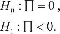
\begin{array}{l} H_{0} : \prod^{​} = 0, \\ H_{1} : \prod^{​} < 0. \end{array}

The null hypothesis (H₀) presents the presence of a unit root (non-stationarity), while the alternative hypothesis (H₁) suggests the time-series variable to be stationary.

Although the unit-root tests can detect the non-stationary behaviour in a time-series variable, the results are sometimes biased towards non-rejection of the unit-root null if there is a structural break (SB) in the series. As the presence of SB might alter the underlying relationship among variables, it might mean that the parameters (such as intercept or trend or both) are not constant over time. This makes it important to identify the presence of SB in the series.

To examine whether SB is present or not, the study followed the method of testing unit root with endogenous break point used by Zivot and Andrews (1992). Here, the null hypothesis (H₀) asserts that the time-series variable contains a unit root along with SB in both intercept and trend terms. Zivot and Andrews (1992) tested it by checking the coefficient (β₁) of the lag of the dependent variable (y_t _{− 1}) in the following regression:

Δ y_{t} = β_{0} + β_{1} y_{t - 1} + δ_{t} + α_{1} D_{1} (\hat{t}) + α_{2} D_{2} (\hat{t}) + \sum_{j = 1}^{p} θ_{j} Δ y_{t - j} + ε_{t} .

(3)

Zivot and Andrews’ (1992) method tests the possibility of a unit root for each possible break point (denoted by ‘t’ in the above equation) and thereafter chooses the break point (tˆ), which gives the least value of the t-statistic calculated for unit roots. Then, the estimated value of the t-statistic is compared against the critical values as developed by Zivot and Andrews (1992).

After carrying out the unit-root test, the study explores the existence of the EKC hypothesis for CO₂ emission in the context of India with the help of co-integration analysis. As the EKC involves time-series data depicting LR dynamics, recent studies have mostly used the co-integration technique to infer the income–pollution relationship. Intuitively, co-integration portrays the LR equilibrium association among the relevant variables. The variables will be in an equilibrium state if their linear combination is stationary.

For analysis, the study has opted for the autoregressive distributed lag (ARDL) approach in the co-integration technique developed by Pesaran et al. (2001). The empirical literature on EKC significantly employed such an ARDL framework when it came to the case of finite small samples (Baek & Kim, 2013; Shahbaz et al., 2012). The traditional co-integration literature talks about the Engle–Granger two-step method, where the residual stationarity provides evidence for co-integration among the relevant variables. In contrast to the Engle–Granger method, the ARDL approach gives the freedom to estimate a model even when the time-series variables are integrated of different orders. Loosely speaking, in the case of the ARDL approach, the vector of time-series variables may contain I(0), I(1), or even a mix of both I(0) and I(1) series. Notably, the ARDL regression equation incorporates both the lagged (past period) dependent (explained) and independent (explanatory) variables as per the Akaike information criterion (AIC), which potentially resolves the endogeneity problem in time-series data. Here, the ARDL approach incorporates a linear formula of lagged (past period) variables, which can act as a representative for the lagged (past period) error-correction term in the Engle–Granger method (Baek & Kim, 2013).

To study the long-run (LR) and short-run (SR) impacts of GDP per capita and FDI on CO₂ emissions, the reduced-form equation is represented in the error-correction model as developed by Pesaran et al. (2001):

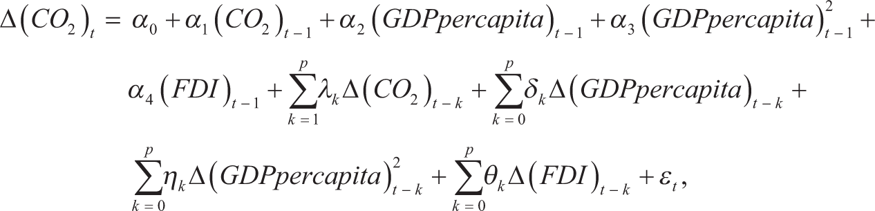
\begin{array}{l} Δ {(C O_{2})}_{t} = α_{0} + α_{1} {(C O_{2})}_{t - 1} + α_{2} {(G D P p e r c a p i t a)}_{t - 1} + α_{3} {(G D P p e r c a p i t a)}_{t - 1}^{2} + \\ α_{4} {(F D I)}_{t - 1} + \sum_{k = 1}^{p} λ_{k} Δ {(C O_{2})}_{t - k} + \sum_{k = 0}^{p} δ_{k} Δ {(G D P p e r c a p i t a)}_{t - k} + \\ \sum_{k = 0}^{p} η_{k} Δ {(G D P p e r c a p i t a)}_{t - k}^{2} + \sum_{k = 0}^{p} θ_{k} Δ {(F D I)}_{t - k} + ε_{t}, \end{array}

(4)

where Δ denotes the first difference, and p indicates the lag length (which is chosen by AIC). The LR dynamics are captured through the coefficients α₁, α₂, α₃ and α₄, and the SR relations correspond to the coefficients λ, δ, η and θ.

Next, to test the presence of co-integration, the study has used the ARDL bound test. In this case, the null hypothesis (H₀) asserts that there is no level (co-integrating) relation among the variables. Mathematically, this can be expressed as

H_{0} : α_{1} = α_{2} = α_{3} = α_{4} = 0.

H₀ is rejected if the estimated value of the F-statistic is greater than the upper-bound (I(1)) critical values. In other words, a sufficiently higher value of the F-statistic indicates the presence of a co-integrating relationship among the variables.

In the case of ARDL models, the existence of autocorrelation can make the SEs biased, which can produce an incorrect estimate of the F-statistic. Also, if autocorrelation is present in the noise (disturbance) term ε_t, it can cause the endogeneity problem. To resolve this, the study has employed the Breusch–Godfrey (BG) test. The BG test is conducted in two stages. In the first stage, the study estimates the ARDL regression equation and calculates the residuals. Next, the estimated residual is regressed in an auxiliary regression equation on all the explanatory variables and the lagged residuals. The null hypothesis (H₀) in this context indicates the presence of no serial correlation against the alternative hypothesis of the presence of serial correlation. A sufficiently higher p value (p > .05) guarantees the non-existence of autocorrelation in the model.

Now, the TP refers to the peak of EKC. Therefore, mathematically speaking, TP indicates the point where the slope is zero when the effect of income on pollution is considered, controlling for other variables.

In the LR, the equilibrium relationship becomes

{(C O_{2})}_{t} = α_{0} + α_{2} {(G D P p e r c a p i t a)}_{t} + α_{3} {(G D P p e r c a p i t a)}_{t}^{2} + α_{4} {(F D I)}_{t} + ε_{t} .

(5)

In this regard, the estimated value of TP can be obtained as follows:

\begin{array}{l} \frac{δ {(C O_{2})}_{t}}{δ {(G D P p e r c a p i t a)}_{t}} = 0 \\ = > α_{2} + 2 α_{3} G D P p e r c a p i t a = 0 \\ = > G D P p e r c a p i t a = - (\frac{α_{2}}{2 α_{3}}) . \end{array}

(6)

\frac{δ^{2} {(C O_{2})}_{t}}{δ {(G D P p e r c a p i t a)}_{t}^{2}} = 2 α_{3} .

(7)

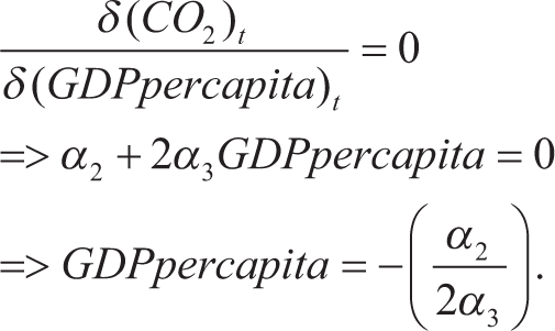
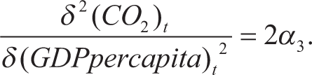
If α₂ > 0 and α₃ < 0, that is, the inverted-U relationship is observed, then the above expression generates a feasible value of TP.

Therefore, it can be readily observed that to the left of TP, the EKC is positively sloped. To the right of TP, the EKC is negatively sloped, and at GDP per capita = –(α₂/2α₃), the curve achieves a maximum.

Empirical Findings

The attempt to infer the pattern of income–pollution dynamics in India is made in four steps. First, the study has plotted the behaviour of all the variables from 1971 to 2021, as shown in Figure 1. It is evident from the graph that CO₂ emission and GDP per capita (and so the square of GDP per capita) share the same kind of stochastic behaviour over time.

Figure 1.

Source: Authors’ estimation.

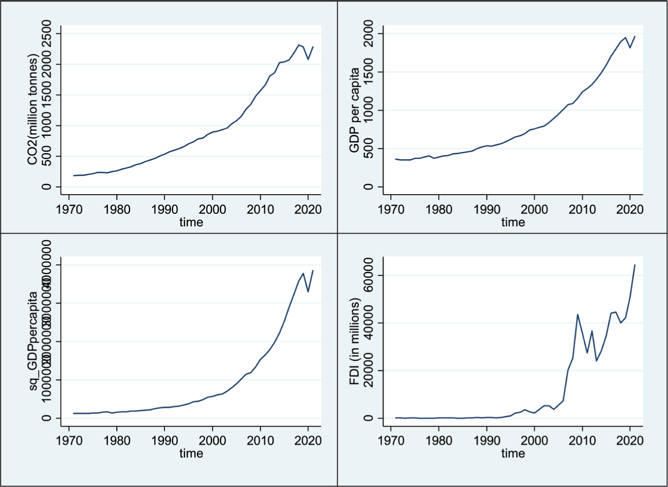
From the 1970s, a clear upward trend can be observed in both GDP per capita and CO₂ emissions, depicting the development trajectory of the Indian economy. However, in the atmosphere of the COVID-19 outbreak, a downfall can be observed. On the other hand, the graph for FDI presents some fluctuations over the timeline (Figure 1), portraying the different trade policy regimes in the pre-liberalisation and post-liberalisation era. Overall, as all the variables here roughly indicate similar patterns of movement over time, it is reasonable to check for the presence of any LR equilibrium relationship among them. In other words, co-movement in the time series acts as a rationale to check for the presence of a co-integrating relationship among them.

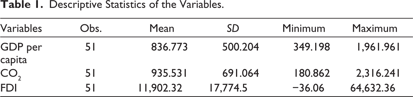
Before diving into the detailed analytical framework, it would be better to first have a look at the summary statistics of the variables presented in Table 1. The yearly mean per capita income is found to be $836.773. Although the country recorded positive improvements in terms of economic growth, it is still lagging in terms of per capita income. The yearly consumption of CO₂ is found to be 935.531 million tonnes. The average foreign investment in India is $11,902.32 million (presented in Table 1).

Table 1.

Descriptive Statistics of the Variables.

Variables	Obs.	Mean	SD	Minimum	Maximum
GDP per capita	51	836.773	500.204	349.198	1,961.961
CO₂	51	935.531	691.064	180.862	2,316.241
FDI	51	11,902.32	17,774.5	−36.06	64,632.36

The trending behaviour of time series acts as a signal for non-stationarity. Therefore, in the second step, the study conducted the Phillips and Perron (1988) test to detect the non-stationarity in the LR. The results from the PP test suggest that all the variables exhibit a different stationary process (DSP) at their level forms. In other words, H₀ cannot be rejected for all the variables at 1% and 5% levels of significance. The results of unit-root tests are provided in the appendix (from Table A1 to Table A8).

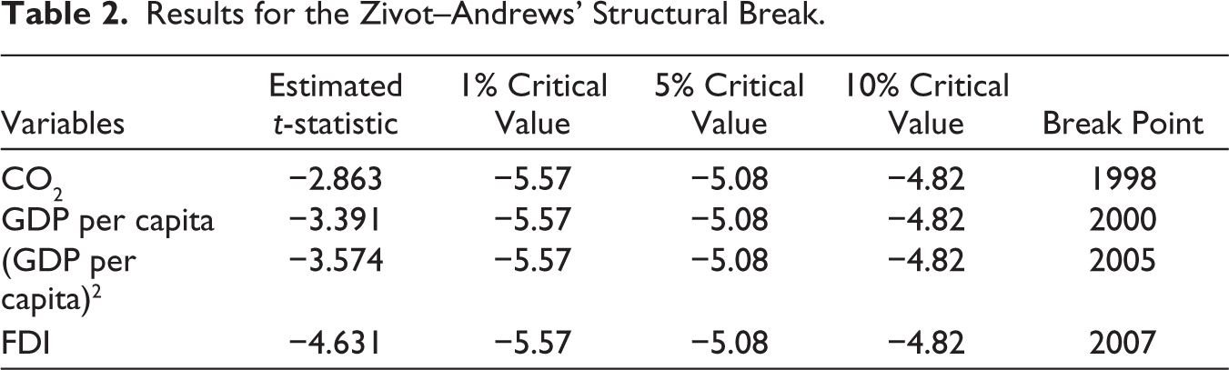
Now, as mentioned in the fourth section, the presence of an SB is tested using the method by Zivot and Andrews (1992). The results in Table 2 indicate that all the variables contain a unit root along with SB (in both intercept and trend terms). Therefore, mathematically, the estimated t-statistic for each of the concerned variables turns out to be smaller than the critical values (in an absolute sense), and thus the study fails to reject the null hypothesis of the presence of non-stationarity and SB. Therefore, all the variables are non-stationary.

Table 2.

Results for the Zivot–Andrews’ Structural Break.

Variables	Estimated t-statistic	1% Critical Value	5% Critical Value	10% Critical Value	Break Point
CO₂	−2.863	−5.57	−5.08	−4.82	1998
GDP per capita	−3.391	−5.57	−5.08	−4.82	2000
(GDP per capita)²	−3.574	−5.57	−5.08	−4.82	2005
FDI	−4.631	−5.57	−5.08	−4.82	2007

No meaningful causal interpretations can be derived until the variables are made stationary. As the variables follow DSP, they can be made stationary by taking the appropriate order of difference. At the first difference, the results suggest that H₀ can be rejected for both 1% and 5% levels. Hence, all the variables are integrated of order one [I(1)], implying the presence of a single unit root. The results of unit-root tests are provided in the appendix (from Table A1 to Table A8).

In the third step, the study used the ARDL model to estimate the LR and SR relations. The results are presented in Table 3. The coefficients of GDP per capita and the square of GDP per capita are positive and negative, respectively, and both are highly significant (at the 1% level). This implies that an inverted U-shaped association exists between GDP per capita and CO₂ emission in the LR. Therefore, with an expansion in economic activities, the pollution (CO₂ emission) would tend to rise initially, but after a threshold income level, the emission is likely to fall. Mathematically, the rate of increase in CO₂ emissions concerning GDP per capita will fall over time, leading to a concave schedule as predicted by the EKC hypothesis. On the other hand, the ceteris paribus effect of FDI on CO₂ emission is found to be significantly positive (at the 1% level). This indicates the possibility of shifting the pollution load from other countries to the home country, which can lead to an increase in CO₂ emissions. In other words, lax environmental standards often act as a comparative advantage for low- and middle-income nations in attracting dirty (pollution-intensive) industries, and this, in effect, raises domestic pollution. This opens up the possibility of the existence of the pollution haven hypothesis in the Indian context.

Table 3.

Results from ARDL Model.

Variables	LR coefficients	SR coefficients	Adjustment coefficient
GDP per capita	2.548*** (0.237)
(GDP per capita)²	−0.000741*** (0.000146)
FDI	0.0110*** (0.00385)
D(GDP per capita)_t		−1.065** (0.498)
D(GDP per capita)²_t		0.000605*** (0.00142)
Δ(FDI)_t		−0.00202** (0.00984)
Δ(FDI)_{t − 1}		−0.00362*** (0.000934)
Constant		−165.5*** (42.51)
(CO₂)_{t − 1}			−0.305*** (0.0794)
R ²		0.850
No. of observations		47

Note: ***p < 0.01, **p < 0.05; SEs are in parentheses.

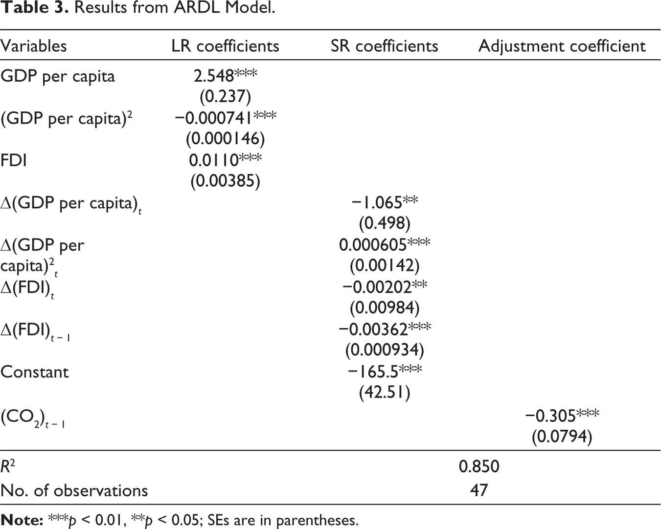
On the other hand, in the SR, the ARDL results exhibit a seemingly different story. From the third column of Table 3, it can be observed that the coefficient of Δ(GDP per capita) is negative, while the coefficient of Δ(GDP per capita²) is positive. Both are significant at 5% and 1% levels, respectively. This exerts a U-shaped relationship in the SR. Intuitively, this implies that initially, as GDP rises (so that Δ(GDP) is positive), the CO₂ emission falls (implying Δ(CO₂) is negative). However, after a threshold level, as the GDP increases, CO₂ emissions also go up. In other words, a sufficiently large growth in GDP per capita raises pollution. This is in contrast with the estimates of the LR as described earlier. The effect of income in the SR can differ from that in the LR. In other words, the short-term fluctuations might deviate from the LR dynamics due to the difference between the pace of industrialisation and the adoption of technology. As income rises, countries might switch from traditional means of production to energy or capital-intensive methods. Since over a shorter span of time, technology cannot grow rapidly, there might be some technological constraints to controlling pollution, such that beyond a specific (threshold) level, a further increase in income causes pollution (Dinda et al., 2000). From an econometric perspective, it can be argued that, as the study observes the presence of an SB in each of the series and an SB can alter the underlying relationship between the variables (implying a change in the direction and magnitude of the parameters), the SR relationships are considerably different from those of LR. This SR behaviour obtained in the present analysis can be called short-term dynamic adjustments that capture the immediate impacts of income growth on pollution growth.

Again, in the case of FDI, the SR depicts a different kind of relationship. In Table 3, the coefficient of ΔFDI is negative and significant at the 5% level. This implies that a growth in FDI reduces CO₂ emissions in the SR. In other words, the SR fluctuations (growth) in FDI can bring about positive improvements in air quality (here, with regard to CO₂). Such a result makes room for the presence of innovation shocks (spillover effects) and sectoral transitions of investment in the SR. Sometimes, an influx of foreign funds in the domestic economy causes the domestic firms to upgrade their production techniques in fear of losing market share. Improved efficiency of local firms brings down the level of pollution and waste generated. However, such an effect is contingent upon the absorptive capacity of the domestic firms (Kathuria, 2000). Again, sometimes, it is also observed that the foreign inflow of funds is tied to some environmental regulation. In such a situation, the government might impose some short-term environmental standards to attract such investments (Thi-Hong Van et al., 2024). The lagged difference in FDI is also found to be negative and significant (at the 1% level), portraying the same result. That is, a short-term positive inflow (here, growth) of FDI in the previous year will result in a reduction in CO₂ emissions in the present period.

Finally, the coefficient of the adjustment term (lag of CO₂) is negative and significant at 1%. This indicates that the effect of any short-term deviation from the LR equilibrium path is transitory, and the system will adjust to the LR equilibrium eventually through the speed of adjustment. Here, the coefficient is found to be −0.305. This implies that the error (disequilibrium) will be corrected by 30.5% in the present period (say, at period t) for any deviation in the immediate past period (say, at period t − 1), and the speed of adjustment is nearly 3.29 years (1/0.305 ≈ 3.29). Therefore, it can be said that the ECM works and the LR association exists. Now, following this notion, it is clear that, although due to the SR fluctuations in GDP per capita, the emission is depicting a U-shaped pattern, such deviation from the LR equilibrium path will be rectified over time. Similarly, for FDI, even though the sudden fluctuations bring about positive environmental benefits, such gains are transitory and will die out over a longer horizon.

In the fourth step, the study employed the ARDL bounds test to check for the existence of co-integration. Also, as the study is based on time-series data, it is also important to test for serial correlation. To detect the presence of autocorrelation, the BG test is executed. The results are presented in Table 4.

Table 4.

Result of the BG and ARDL Bound Test.

χ² (1)	0.558 (0.4550)
F-statistic	15.083***
t-statistic	−3.839**

Note: The p value for χ² is provided in parentheses. The 1% critical value for the F-statistic is 5.61; the 5% critical value for the t-statistic is −3.78. **p < 0.05 and ***p < 0.01.

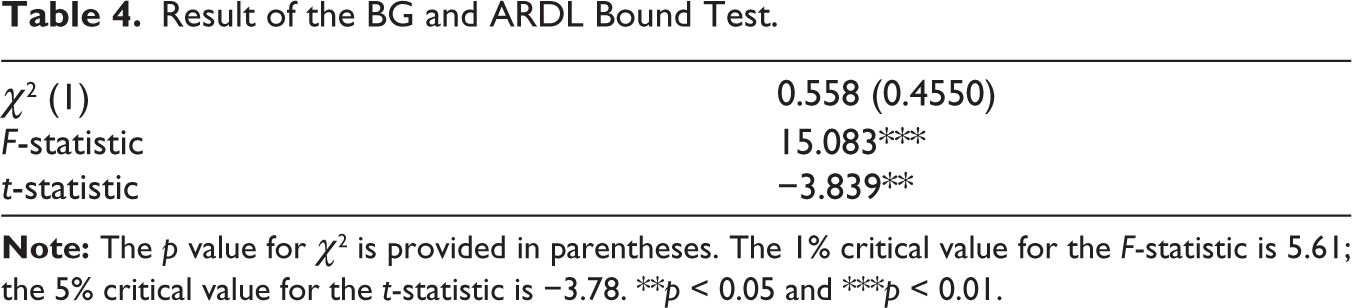
It is evident from Table 4 that the estimated F-statistic signifying the joint significance of the LR coefficients is found to be 15.083, which is much higher than the I(1) bounds at the 1% critical value. Thus, the null hypothesis of no co-integration (no level relationship) can be rejected at the 1% level of significance. In other words, the test results indicate that co-integration exists among the concerned variables. Again, the calculated t-statistic (−3.839) is lower than I(1) bounds at the 5% level. Therefore, the null hypothesis concerning no influence of the lagged dependent variable can be rejected at the 5% level of significance. This ensures that the ECM works and thus guarantees a stable relationship over time.

As the variables tend to move on an inverted U-shaped path in the LR, it would be very contextual to estimate the value of the TP. The result finds that the Indian economy will achieve its TP concerning CO₂ emission at $1,719.513 per capita, which is comparatively lower than other countries’ context (Agras, 1995; Shafik & Bandyopadhyay, 1992). However, as the obtained value of TP lies within the sample range, it provides feasible and justified evidence towards the presence of EKC in the Indian context. Notably, the estimated threshold value (TP) is a sample-based estimate, which can vary empirically and thus cannot be generalised for India over different time spans. However, from the Indian experience, it can be strongly argued that most of the manufacturing activities, such as burning fuel and gases, cause CO₂ emissions. As the formal manufacturing sector in the country did not flourish after the 1990s (Gupta & Kumar, 2010), and as the data on the true size of the informal sector are difficult to obtain for a longer period, the estimate of TP has come out to be low.

Conclusions

By taking CO₂ emission as an environmental degradation indicator and GDP per capita as the income measure, the present study examines the validity of the EKC for the Indian economy. Considering the reduced-form econometric model, the results find significant evidence for the LR presence of EKC for CO₂ emission in India during 1971–2021, while acknowledging the SB as found in the works of Baek and Kim (2013), Jalil and Mahmud (2009), Ozturk and Acaravci (2013), Shahbaz et al. (2010) and Shahbaz et al. (2012) for countries like Korea, China, Turkey, Portugal and Pakistan, respectively. However, this is in contrast to the findings reported for some developed countries, such as Germany and OECD countries, where an N-shaped or monotonically increasing curve is found (Egli, 2004; Lieb, 2003; Liu, 2005).

The bell-shaped association between CO₂ emission and GDP per capita for the country intuitively projects the underlying structural transformation in an economy. The rapid growth of manufacturing activities creates severe environmental damage during the initial phases of economic development. As income and standard of living improve, later on, diversification can be observed in both production and consumption bundles. The production activities get switched from dirty pollution-intensive technology to modern, cleaner technology. Again, as environmental quality has an income elasticity of more than one (Dinda, 2004), consumers also prefer to have greener products at the expense of dirty polluted products. All these effects may result in a reduction in pollution levels.

However, India’s growth experience is slightly different from that of many other countries. For India, there has been a rapid growth of the modern service sector since liberalisation, while the growth of the manufacturing sector has remained relatively stagnant (Gupta & Kumar, 2010). Although the service sector generated demand for a skilled labour force, the unskilled and semi-skilled workers were mostly absorbed in informal activities (Dev, 2000; Naik, 2009). Therefore, in the context of the Indian economy, it may be the informal sector that contributes to the rising part of the EKC. The estimated value for TP for CO₂ emission is found to be $1,719.513 per capita, which seems to be relatively lower but feasible as per the sample observations.

By employing the ARDL framework, the current study has notably observed that the SR effects are quite different from the LR impacts, which is unlike many of the findings in EKC literature (Baek & Kim, 2013; Shahbaz et al., 2012). Over shorter intervals, sudden fluctuations in GDP per capita are found to influence the CO₂ emission in a non-linear (U-shaped) fashion. This is indicative of the presence of SBs or technological constraints in abating pollution in the SR (Dinda et al., 2000). However, such deviation from the LR equilibrium relation is short-lived.

Coming to the effect of FDI on CO₂ emission, the presence of the pollution haven hypothesis is found, which is aligned with the findings by Acharyya (2009), Bello and Adenyi (2010), Rana and Sharma (2019), Solarin et al. (2017), etc. However, although FDI is detrimental for the environment over the long term, the SR effects are contradictory. Over a shorter span, the higher growth in FDI flow will favour the possibility of innovation shocks (spillover effects) and short-term stringency in environmental standards, resulting in lesser pollution (Kathuria, 2000; Thi-Hong Van et al., 2024). However, such short-term benefits are transitory and will eventually shrink in the LR.

From the Indian experience, it can be observed that several initiatives (such as ‘National Clean Air Programme (NCAP)’ and ‘Net Zero Carbon Emission Target of 2070’) are aimed at reducing emissions, but the country still ranks in the top three positions in global CO₂ emissions. Such evidence inherently suggests that policy efforts are backfiring on the system with rebound effects over the shorter span. The policy initiatives can actually influence the relationship between income and pollutants (Lieb, 2003). It is also important to incorporate public reaction to environmental deterioration in policy formulations (Perrings & Ansuategi, 2000). Hence, it opens up room for cautious policy formulation in the sense that while designing any policy, policymakers need to take care of the long-term impact, rather than focusing only on the short-term benefits or costs.

Finally, the results obtained in this study cannot be generalised for all pollutants. As the income–pollution dynamics are pollutant-specific as well as cross-section-specific, the findings can be expected to vary across pollutants and nations. In other words, the income–pollution relationship is more often driven by the nature and the availability of data (Lieb, 2003). Therefore, specific policy prescriptions are required for specific pollutants in each country to help reduce the overall pollution level.

Footnotes

Acknowledgements

The authors are grateful to the anonymous reviewers for their valuable comments in improving this article.

Declaration of Conflicting Interests

The authors declared no potential conflicts of interest with respect to the research, authorship and/or publication of this article.

Funding

The authors received no financial support for the research, authorship and/or publication of this article.

Appendix

Table A10.

Regression Results for CO₂ on FDI.

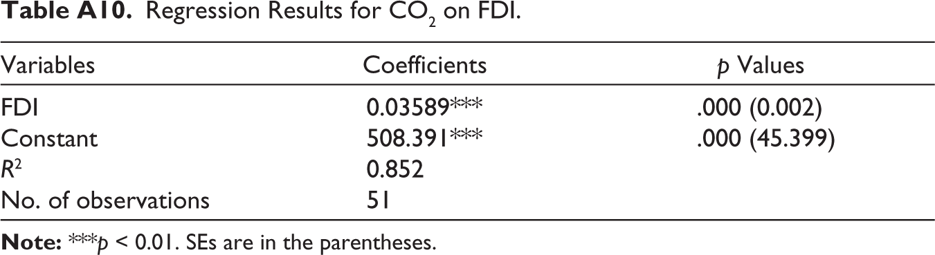
Variables	Coefficients	p Values
FDI	0.03589***	.000 (0.002)
Constant	508.391***	.000 (45.399)
R ²	0.852
No. of observations	51

Note: ***p < 0.01. SEs are in the parentheses.

References

Abbasi

M. A.

, Nosheen

, & Rahman

H. U.

(2023). An approach to the pollution heaven and pollution Halo hypotheses in Asian countries. Environmental Science and Pollution Research, 30, 49270–49289. https://doi.org/10.1007/s11356-023-25548-x

Acharyya

(2009). FDI, growth and the environment: Evidence from India on CO₂ emission during the last two decades. Journal of Economic Development, 34(1), 43–58.

Agras

(1995). Environment and development: An economic analysis of pollution, growth and trade [Master’s thesis, Department of Agriculture, Resource, and Managerial Economics, Cornell University].

Agras

, & Chapman

(1999). A dynamic approach to the environmental Kuznets curve hypothesis. Ecological Economics, 28, 267–277. https://doi.org/10.1016/S0921-8009(98)00040-8

Auty

(1985). Materials intensity of GDP: Research issues on the measurement and explanation of change. Resource Policy, 11, 275–283. https://doi.org/10.1016/0301-4207(85)90045-5

Baek

, & Kim

H. S.

(2013). Is economic growth good or bad for the environment? Empirical evidence from Korea. Energy Economics, 36, 744–749. https://doi.org/10.1016/j.eneco.2012.11.020

Bardhan

, Debnath

, & Jana

(2019). Evolution of sustainable energy policies in India since 1947: A review. WIREs Energy Environment, 8, 1–16. https://doi.org/ 10.1002/wene.340

Beckerman

(1992). Economic growth and the environment: Whose growth? Whose environment? World Development, 20, 481–496. https://doi.org/10.1016/0305-750X (92)90038-W

Bello

, & Adenyi

(2010). FDI and the environment in developing economies: Evidence from Nigeria. Environmental Research Journal, 4(4), 291–297.

10.

Dev

S. M.

(2000). Economic liberalisation and employment in South Asia – I. Economic & Political Weekly, 35(1/2), 40–51. https://www.epw.in/journal/2000/01-02/special-articles/economic-liberalisation-and-employment-south-asia-i.html

11.

Dinda

(2004). Environmental Kuznets curve hypothesis: A survey. Ecological Economics, 49, 431–455. https://doi.10.1016/j.ecolecon.2004.02.011

12.

Dinda

, Coondoo

, & Pal

(2000). Air quality and economic growth: An empirical study. Ecological Economics, 34, 409–423.

13.

Egli

(2004). The environmental Kuznets curve – Evidence from time-series data for Germany (Economics Working Paper Series 03/28). ETH Zurich, CERETH – Center of Economic Research, Zurich. https://www.econstor.eu/bitstream/10419/171472/1/wp-03-028_rev.pdf

14.

Ehrlich

P. R.

, & Ehrlich

A. H.

(1991). Population growth and environmental security. The Georgia Review, 45(2), 223–232. https://www.jstor.org/stable/41400160

15.

Grossman

G. M.

, & Krueger

A. B.

(1991). Environmental impacts of North American free trade agreement [Working paper no. 3914, National Bureau of Economic Research].

16.

Grossman

G. M.

, & Krueger

A. B.

(1995). Economic growth and the environment. The Quarterly Journal of Economics, 110(2), 353–377.

17.

Gupta

, & Kumar

(2010). Performance of Indian manufacturing in the post reform period. SSRN. https://papers.ssrn.com/sol3/papers.cfm?abstract_id=1608663

18.

Gupta

, Biswas

, & Ganesan

(2017, September 1). Greenhouse gases emission estimates from the manufacturing industries in India state level estimates: 2005 to 2013. GHG Platform India Report. https://www.ceew.in/publications/state-and-sector-wise-greenhouse-gases-and-carbon-emissions-india

19.

Holtz-Eakin

, & Selden

T. M.

(1995). Stocking the fires? CO₂ emission and economic growth. Journal of Public Economics, 57, 85–101. https://doi.org/10.1016/0047-2727(94)01449-X

20.

Inampudi

, & Gaurav

A. K.

(2024). Transforming institutions for inclusive and sustainable governance: An empirical analysis of NITI Aayog’s role in India. In Zafarullah

& Azmat

(Eds), Governance and sustainable development in South Asia. South Asian Public Administration. https://doi.org/10.1007/978-3-031-67616-1_10

21.

International Energy Agency. (2021). India energy outlook 2021. https://iea.blob.core.windows.net/assets/1de6d91e-e23f-4e02-b1fb-51fdd6283b22/India_Energy_Outlook_2021.pdf

22.

Jalil

, & Mahmud

S. F.

(2009). Environmental Kuznets curve for CO₂ emissions: A cointegration analysis for China. Energy Policy, 37, 5167–5172. : https://doi.10.1016/ j.enpol.2009.07.044

23.

Kathuria

(2000). Productivity spillovers from technology transfer to Indian manufacturing firms. Journal of International Development, 12, 343–369.

24.

Kijima

, Nishide

, & Ohyama

(2010). Economic models for the environmental Kuznets curve: A survey. Journal of Economic Dynamics and Control, 34(7), 1187–1201. https://papers.ssrn.com/sol3/papers.cfm?abstract_id=1601176

25.

Lieb

C. M.

(2003). The environmental Kuznets curve: A survey of empirical evidence and possible causes [Discussion paper no. 391, University of Heidelberg, Department of Economics, Heidelberg].

26.

Liu

(2005). Explaining the relationship between CO₂ emissions and national income – The role of energy consumption. Economic Letters, 87, 325–328. https://doi.10.1016/j.econlet.2004.09.015

27.

Mert

, & Caglar

A. E.

(2020). Testing pollution heaven and pollution halo hypothesis for Turkey: A new perspective. Environmental Science and Pollution research, 27, 32933–32943. https://doi.org/10.1007/s11356-020-09469-7

28.

Ministry of Coal. (2023). Energy cell monthly report. Government of India.

29.

Naik

A. K.

(2009). Informal sectors and informal workers in India. Special IARIW-SAIM Conference on Measuring the Informal Economy in Developing Countries.

30.

Ozturk

, & Acaravci

(2013). The long run and causal analysis of energy, growth, openness and financial development on carbon emissions in Turkey. Energy Economics, 36, 262–267. https://doi.org/10.1016/j.enpol.2012.08.065

31.

Panayotou

(1993). Empirical tests and policy analysis of environmental degradation at different stages of economic development. International Labor Organization, Technology and Employment Programme, Geneva. https://webapps.ilo.org/public/libdoc/ilo/1993/93B09_31_engl.pdf

32.

Panayotou

(2000). Economic growth and the environment [Working Paper No. 56]. Center for International Development, Harvard University. https://www.hks.harvard.edu/sites/default/files/centers/cid/files/publications/faculty-working-papers/056.pdf

33.

Perrings

, & Ansuategi

(2000). Sustainability, growth and development. Journal of Economic Studies, 27(1/2), 19–54. https://doi.org/10.1108/EUM0000000005309

34.

Pesaran

M. H.

, Shin

, & Smith

R. J.

(2001). Bounds testing approaches to the analysis of level relationships. Journal of Applied Econometrics, 16(3), 289–326. https://www.jstor.org/stable/2678547

35.

Phillips

P. C. B.

, & Perron

(1988). Testing for a unit root in time series regression. Biometrika, 75(2), 335–346. https://doi.org/10.1093/biomet/75.2.335

36.

Rana

, & Sharma

(2019). Dynamic causality testing for EKC hypothesis, pollution haven hypothesis, international trade in India. The Journal of International Trade and Economic Development, 28(3), 348–364. https://doi.org/10.1080/09638199.2018.1542451

37.

Shafik

, & Bandyopadhyay

(1992). Economic growth and environmental quality: Time-series and cross-country evidence. World Development Report, the World Bank. https://documents1.worldbank.org/curated/en/833431468739515725/pdf/multi-page.pdf

38.

Shahbaz

, Jalil

, & Dube

(2010). Environmental Kuznets curve (EKC): Time series evidence from Portugal. Munich Personal RePEc Archive, 27443. https://mpra.ub.uni-muenchen.de/27443/

39.

Shahbaz

, Lean

H. H.

, & Shabbir

M. S.

(2012). Environmental Kuznets curve hypothesis in Pakistan: Cointegration and Granger causality. Renewable and Sustainable Energy Reviews, 16, 2947–2953. https://doi.10.1016/j.rser.2012.02.015

40.

Solarin

S. A.

, Al-Mulali

, Musah

, & Ozturl

(2017). Investigating the pollution haven hypothesis in Ghana: An empirical investigation. Energy, 124, 706–719. https://doi.org/10.1016/j.energy.2017.02.089

41.

Thi-Hong Van

, Vo

D. H.

, Vu

N. T.

, Ho

C. M.

, & Nguyen

T. C.

(2024). From foreign direct investment to environmental regulations: Does a feedback effect ever exist? Heliyon, 10, 1–14. https://doi.org/10.1016/j.heliyon.2024.e28657

42.

Timilsina

R. R.

, Rahut

D. B.

, Gautam

M. S.

, Mishra

, & Sonobe

(2023). Are households shifting toward cleaner cooking fuel? Empirical evidence from India during 2005–2021. Frontiers in Environmental Economics, 2, 1–13. https://10.3389/frevc.2023.1137248

43.

Zhang

, & Guo

(2024). Attracting private investment to renewable energy projects in India. Utilities Policy, 90, 101816. https://doi.org/10.1016/j.jup.2024.101816

44.

Zivot

, & Andrews

D. W. K.

(1992). Further evidence on the great crash, the oil-price shock, and the unit-root hypothesis. Journal of Business & Economic Statistics, 10(3), 251–270. https://10.1080/07350015.1992.10509904