
Abstract
Linear discriminant analysis (LDA) has found extensive application in predicting bankruptcy. In this article, we elucidate a novel modelling approach for LDA that can also aid in gaining useful insights regarding the relative importance and ranking of factors in the banking industry. The model steers away from the traditional computation of the variance/covariance matrix and employs an ensemble technique to assign records to classes. The efficacy of our model is tested using two datasets. Specifically, a large dataset from the banking industry was partitioned into the testing and training datasets, and an accuracy of 87.9% was achieved
Keywords
Introduction
The linear discriminant analysis (LDA) was developed by Fisher (1936), considered by many as the father of modern statistics (Read, 2016). The purpose of LDA was to delineate two or more populations based on their characteristics x1, x2, x3, …, xk using a linear function Z = a1x1+ a2x2 + a3x3 + … + akxk. The linear function, also known as the linear discriminant function, is a linear combination of the characteristics that are used to discriminate between groups. Consequently, discriminant analysis can be described as a statistical tool employed to discriminate/separate two or more categories of a dependent variable using linear discriminant functions (or hyperplanes) that are linear combinations of the independent variables.
Other popular competing statistical tools used in classification and multivariate statistical testing include the T-square distribution (Hotelling, 1931), Mahalnobis distance (Mahalanobis, 1936), logistic regression (Gaja & Liou, 2018; Johnson et al., 2018), neural networks (Gaja & Liou, 2018; Li et al. 2018), and support vector machines (SVM) (Venkatesan et al., 2018; Wang et al., 2018). While the T-square distribution, a generalization of the student’s t-test, is used in multivariate statistical testing, the Mahalanobis distance finds applications in cluster analysis and classification techniques for face and pattern recognition (Li et al. 2018; Mohammed et al. 2018).
Logistic regression (Cramer, 2004) is a powerful and versatile tool as the independent variables need not be normally distributed (Pohar et al., 2004). The neural network was first explored by Rosenblatt (1962) as a classification tool in 1962. It consists of interconnected neurons where each neuron represents a separating hyperplane. Therefore, the network represents piecewise linear separating hyperplanes. Other early literature on neural networks includes the work of Rumelhart et al. (1986, 1987). SVM (Cortes & Vapnik, 1995; Hastie et al., 2008) focusses on constructing a hyperplane or a set of hyperplanes that tries to maximize the distance from the hyperplane to the nearest data point of the other class.
Despite the availability of several alternate techniques for classification problems, LDA remains a very useful tool in the world of statistical analysis and statistical modelling. Some of the applications of LDA include (a) solving spatial problems (King, 1970; Unsal & Nazman 2020), (b) biology and biological studies (David et al., 2010; Maroco et al., 2011; Morais & Lima, 2018; Preisner et al., 2010; Rao, 1948), (c) pattern recognition (Fard et al., 2018; Jayadevan et al. 2011; Liu et al., 2004; Peets et al. 2017; Siddiqi et al., 2015; Zeina & Al-Anzi, 2018), (d) textile industry (Vila & Kuster, 2007) and (e) bankruptcy prediction (Altman, 1968, 1984; Cardwell et al., 2003; Samarakoon & Hasan, 2003; Viswanathan et al., 2020).
Given the established profound significance of LDA in statistical analysis, it is highly imperative to build a strong foundation in understanding this modelling technique by simple practical means. The traditional method of teaching LDA in a classroom assumes advanced knowledge of linear algebra on the part of the participants (Ragsdale & Stam, 1992). Our modelling approach maintains the spirit of Fisher by focussing on maximizing the distance between the group centroids with a constraint that the pooled variance is equal to one. The modelling approach draws some basic ideas from the spreadsheet models developed by Albright and Winston (2009).
We also present a generalized approach that can model more than two groups. In this scenario, we consider two groups at a time (pairwise) with common variance, ensemble the predictions of all pairwise comparisons, and then take a maximum vote approach for prediction of classes. Although such an approach is practised in other machine learning models like SVM, we have not come across such an approach (in practise) for LDA to the best of our knowledge.
Additionally, we also study the relative importance of factors for each pairwise comparison, and then use them to rank order the factors in the overall scheme of things. We consider this a key contribution of our article as this information can be used to reduce the number of variables needed in the study.
The rest of the article is as follows. Section 2 presents a review of the applications of LDA in studying banking and financial industries. Section 3 presents the detailed algorithm for our modelling approach that extends the discriminant analysis to more than two groups. Section 4 presents the case analysis using two datasets from the finance/banking industry, and the conclusions are presented in Section 5.
Application of LDA in Financial and Banking Sectors
LDA finds applications in bankruptcy prediction based on accounting ratios and other financial variables. The seminal article by Altman (1968) to predict corporate bankruptcy considered 66 manufacturing corporations, of which 50% were bankrupt and the rest were solvent. Altman’s model (Altman, 1968) is still useful in many practical situations, although LDA’s fundamental assumption of normal distribution for the independent variables may not always hold true for financial ratios.
Several modelling efforts have focussed on improvising the Z-score model. Altman et al. (1977) developed the Zeta model that had seven variables and considered accounting adjustments. Springate (1978) initially considered 19 financial ratios, but after refinement, settled for only four ratios to determine the health of the company. Altman’s Z-score and its modifications have found applications in bankruptcy prediction in the steel industry (Altman, 1993), savings and loan associations (Pantalone & Platt, 1987), railroads (Altman, 1983), retail sales (Nunthapad, 2000), textile industry (Cardwell et al., 2003), cement industry (Mohammed, 2016; VenkataRamana et al., 2012), and in studying emerging stock markets (Samarakoon & Hasan, 2003). A review of different empirical failure classification models across multiple countries was presented in Altman (1984). A detailed review of bankruptcy prediction studies since the 1930s is presented in Gissel et al. (2007).
There are several studies that consider a comparative analysis of different bankruptcy prediction models. Kiyak and Labanauskaite (2012) study the practical application of bankruptcy prediction models that employ discriminant analysis and logistic regression. The study concluded that LDA-based methods like Altman’s model and Springate’s model performed better than their logistic regression counterparts. A similar comparison was also made by Bunyaminu and Issah (2012), and their conclusion was that the LDA-based methods had a higher accuracy in the first year prior to failure. Husein and Pambekti (2014) compared four different models—two LDA-based models (Altman’s model and Springate’s model), probit-based Zmijewski’s model and Grover’s model. The study concluded that all the models perform well in bankruptcy prediction, while the probit based Zmijewski’s model is the best. Viswanathan et al. (2020) used an unsupervised machine learning technique (k-means clustering technique) to identify logical groups in terms of financial health, and then used supervised learning techniques like LDA and random forest methods for predicting. The study achieved a 95% accuracy with both LDA and random forest and concluded that the LDA is a better alternative as it also has explanatory powers on the relative importance of the variables.
Given the applications of LDA and its variants in the finance/banking domain, in this article, we develop a novel modelling approach for LDA, and highlight details of how the relative importance of variables can be obtained. This is a major contribution to our study.
Novel Modelling Approach for Linear Discriminant Analysis
The traditional approach requires the computation of two p × p variance-covariance matrices (between-class and within-class) followed by the optimization of the ratio of between sum of squares to within sum of squares to obtain various
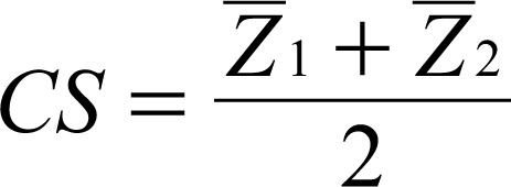
Ragsdale and Stam (1992) developed a regression-based model that worked very well for two group problems. In fact, the results obtained by solving the ordinary least square (OLS) are equivalent to Fisher’s LDA (Fisher, 1936; Ragsdale & Stam, 1992). Their approach considers a problem with two groups, say groups 1 and 2. The dependent variable Z, representing the group variable, is expressed in terms of its n characteristics, say x1, x2, x3, …, xn. The regression equation would then be Z = a + b1x1+ b2x2 + b3x3 + … + bkxk. Note that Z would take the values 1 and 2. The coefficients of the regression equation were then estimated using an OLS regression. The resulting equation was then used to estimate the discriminant score, Z, for each record. The group averages, Z1 and Z2, were calculated, and the average of these two values was chosen as the cut-off point. According to the classification rule, those records with discriminant scores of less than the cut-off point are classified as belonging to group 1, while other records belonged to group 2. However, Ragsdale and Stam (1992) noted the regression model
cannot, in general, be used for DA problems with more than two groups since the relationship between the dependent and independent variables may not be linear. Even if this relationship can be made linear by some appropriate coding for the dependent variable, it can be impossible to discern what this coding should be if there are several independent variables.
Subsequently, Albright and Winston (2009) devised a new algorithm that keeps Fisher’s idea intact while avoiding advanced linear algebra altogether. In their solution methodology, they tried to define a discriminant score for each record i, which was obtained as a linear combination of the discriminant weights and the value of the predictor variable for each record. A record was deemed to be belonging to group k if the discriminant score for record i exceeded the cut-off score. Albright and Winston (2009) solved this problem as an optimization model using the evolutionary solver in Excel. The objective of the model was to maximize the percentage of correct predictions subject to constraints on the discriminant weights (between −1 and +1) and the cut-off point (chosen arbitrarily). The authors note that a drawback to this approach is that each run of the model could potentially return different sets of optimal values for discriminant weights.
To address this drawback, we present the following model to solve LDA. The basic idea is explained in Section 3.1, and the detailed procedure is presented in Algorithm 1.
Some Simple Basics to understand the Goal
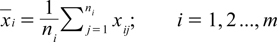
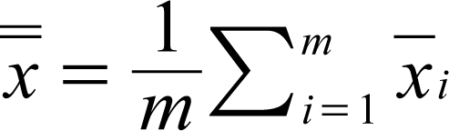
Let an (ni ◊ p) matrix Xi represent a sample drawn from population i. Let the jth row of this matrix be denoted as xij; i = 1, 2, …, m; j = 1, 2, …, ni where m represents the number of groups or populations, ni represents the sample size drawn from population i, and p represents the number of features for each group. Let N be the total number of records. Then we have N = n1 + … + nm. The first step in the procedure involves the computation of the (m ◊ p) vector representing the sample mean,
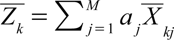
The equation of the hyperplne obtained from LDA can be represented as shown in Equation (3).

where Zi is the determinant score of the record i. Let
Let variance of Z be denoted as Var (Z). Since one of the key goals of the LDA is to maximize the distance between the means/centroids of each group, we solve an optimization model to find the values of a
The decision variables in our model are the discriminant weights. We begin the procedure by calculating the group mean for each predictor variable using Equation (1). The discriminant score is then obtained as the weighted (linear) combination of the predictor variables for each record using the discriminant weights as shown in Equation (3). Note that this calculation is also used by Albright and Winston (2009). The mean discriminant score is then calculated using Equation (4). The group variances are calculated first followed by the calculation of the pooled variance, Var (Z), using Equation (5). Note that Equation (5) furnishes a more generalized formula that can also work for more than two groups. We then use the generalized reduced gradient non-linear method in the Excel solver to obtain the unique discriminant values by maximizing
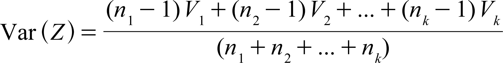
where V1, V2, …, V k , are the group variances for groups 1, 2, …, k, respectively.
Another significant contribution of our approach is that we quantify the relative importance of predictor variables in terms of group separation and classification using the Karl Pearson correlation coefficient between the discriminant score and each input variable.
Algorithm 1 works in the case of two group classification problems. However, when it gets to three or more groups, we resort to the ensemble method, using the maximum voting. Here we perform pairwise comparisons, where each group is separately compared against the rest. Once all comparisons are completed, we count the number of times each group has been predicted for a specific record, and the group with the maximum count (votes) is selected as the group in which that record is classified. Therefore, Algorithm 2 presents the more generic procedure to solve LDA with three or more groups.
Algorithm 1. Modelling Approach for Two Group LDA
Record i belongs to group 1
Record
Having provided the generic algorithm, we are ready to test our model by employing the generalized reduced gradient nonlinear method in MS Excel Solver. In this study, two datasets were used. The first dataset dealt with a two-group classification problem from Altman (1968). The second dataset, a large one with 583 records with three groups from the banking sector, was adopted from the work of Viswanathan et al. (2020). We split the dataset into an 80% training set and a 20% testing set. The detailed implementation of our algorithms using Excel screenshots is presented in Appendix A.
Algorithm 2. Ensemble Technique for Multiclass LDA
Run Algorithm 1 (group k vs k' group)
Votes (i, k) = Votes (i, k) + 1
Group (i) = k
Altman’s Classification Model for Bankrupty Detection among Companies
The seminal article by Altman (1968) classified and predicted corporate bankruptcy based on a set of financial ratios. Z-score of Fisher’s LDA was employed to classify the firm as either “Bankrupt” or “Solvent.” The data used in the study was from manufacturing corporations. The data set has 33 bankrupt firms and 33 solvent firms. The central goal was to determine whether bankrupt firms and solvent firms could be sharply differentiated (separated) in terms of five financial ratios—(a) Working Capital/Total Assets (WCTA), (b) Retained Earnings/Total Assets (RETA), (c) Earnings Before Interest and Taxes/Total Assets (EBITTA), (d) Market Value of Equity/Book Value of Total Debt (MVEBVTD), and (e) Sales/Total Assets (SATA). The abbreviations within brackets are made for ease of identifying the ratios in the spreadsheet columns (see Appendix A). The data set was taken from Morrison (1976).
Discussion of Results
The linear discriminant score function, Z, is presented in Equation (7). The coefficients in the equation are the optimized values of a1, a2, …, a5. These are the weights attached to the five financial ratios taken to differentiate the groups, “Bankrupt” and “Solvent.”

Please note that the coefficients/weights are given to four decimal places for display.
Based on the mean discriminant scores of the two groups, the cut-off score value is 1.1489. If the discriminant score of the individual record is <1.1489, the company is classified as “Bankrupt”, else “Solvent.”
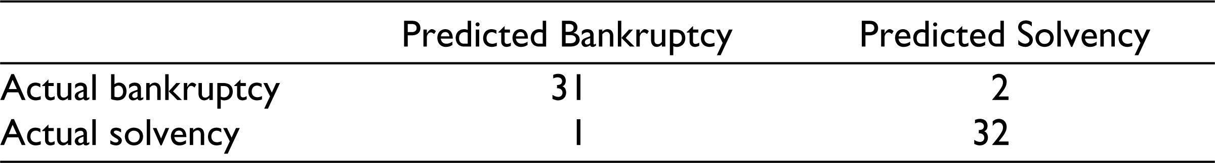
From the prediction made, we see that 63 out of the 66 records have been correctly classified, indicating an accuracy of 95.45%. Given that the actual number of bankrupt companies is 33, the model could predict 31 correctly and misplace 2 into the solvent category. Likewise, given that 33 companies are solvent; the model could predict 32 correctly while misplacing 1 into the bankrupt category. It appears that the discriminant scoring model of Fisher has been able to sharply differentiate “Bankrupt” companies from “Solvent” companies in a robust manner with excellent predictive accuracy. The confusion matrix is presented in Table 1.
Confusion Matrix for Altman’s Data
Having established the model accuracy, we focus on the relative importance of the predictor variables. The relative importance cannot be based on the weights as they behave exactly like the slopes of the regression equation. We instead use the absolute value of the Karl Pearson correlation coefficient between the discriminant score and each input variable to understand the relative importance of the predictor variables (see Table 2 for details).
Relative Importance of the Predictor Variables
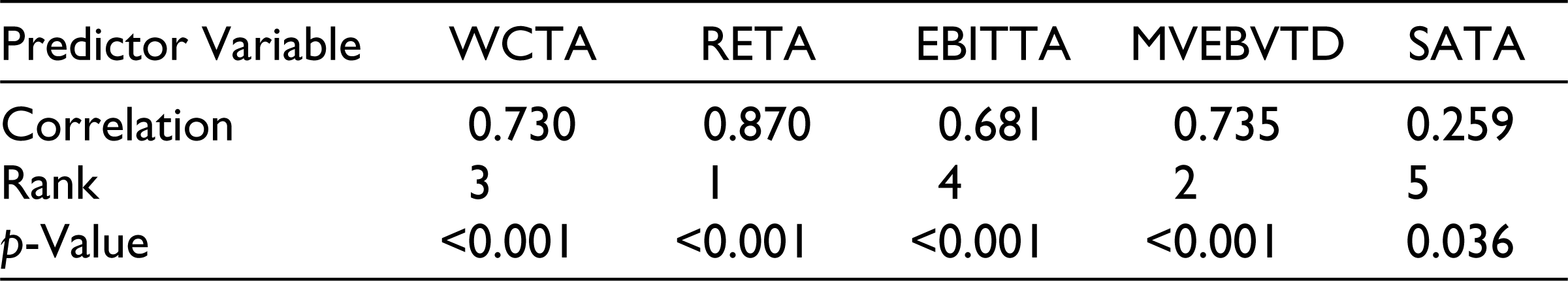
RETA is No. 1, MVEBVTD is No. 2, closely followed by WCTA (No. 3), EBITTA is No. 4, and SATA is No. 5 in terms of relative importance ranking. These rankings are devoid of the influence of the original scale of input variables (in other words, they are invariant to the measurement scale). Except SATA, all the rest are strongly correlated with the discriminant function. A hypothesis test was also conducted to see if there is a significant correlation between the discriminant score and the individual variables. The test showed that all variables are significant (p-values are presented in Table 2). The inference is that these financial ratios, in an emphatic manner, differentiate the two classes sharply and hence serve as good predictor variables of “Bankruptcy”/“Solvency.”
The three-way classification problem on bank data adopted by Viswanathan et al. (2020) classified bank’s health as low, medium or high based on credit-deposit ratio (CDR), ratio of net interest income to total assets (NITA), return on assets (ROA), capacity adequacy ratio—Tier I (CART1), capacity adequacy ratio—Tier II (CART2), liquidity asset to total asset ratio (LATA) and gross nonperforming assets to gross advances ratio (GNPATA). The unbalanced dataset was comprised of 583 records (banks), out of which 133 banks were of low health, 363 banks were of medium health and the remaining 87 were of high health. The central goal was to determine whether the three groups based on the bank’s health (low/group 1, medium/group 2, and (high/group 3) could be sharply differentiated (separately) in terms of the predictor variables listed above. While the Altman’s (1968) dataset was run only in the training mode (given the number of records in this dataset), we split the dataset into training (80% or 467 records) and testing (20% or 116 records) datasets to test the efficacy of the model in classifying new records.
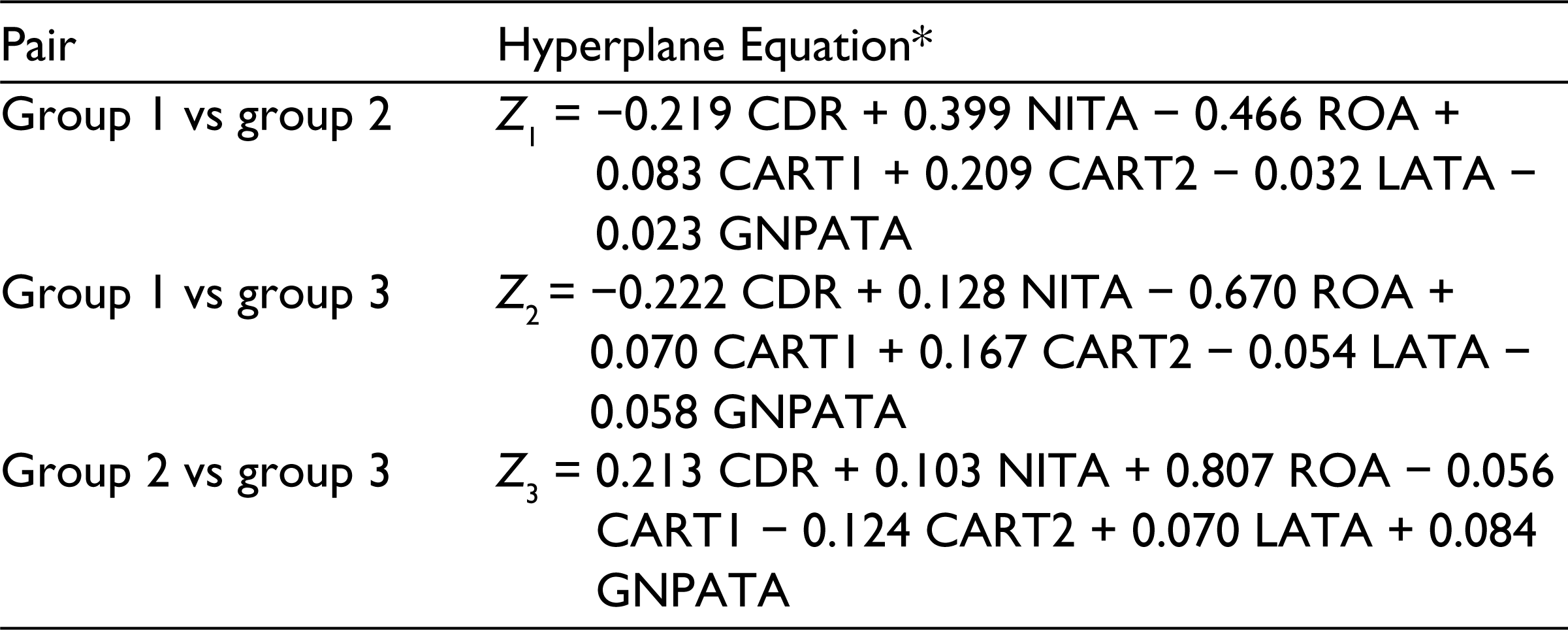
In the solution procedure, we solved three pairwise classification problems for the training set and used the voting procedure (Algorithm 2) to measure the accuracy of our training model. The cut-off scores and the hyperplane equations for the training model are presented in Tables 3 and 4, respectively (see Supplementary Excel files Bank-Train-Solver.xls for training data and results, and Bank-Test-Solver.xls for testing data and results).
Cut-off Scores for the Pairwise Group Classification
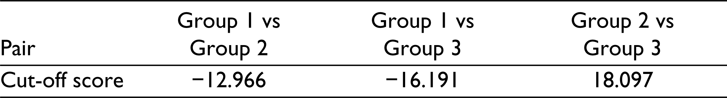
Cut-off Scores for the Pairwise Group Classification
Hyperplane Equation for the Three Pairwise Classification Problem
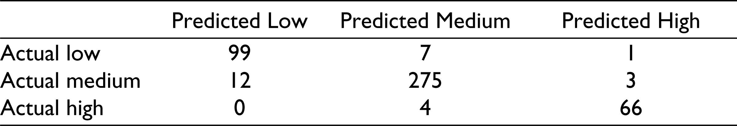
The confusion matrix for the training model is presented in Table 5. The accuracy of the training model was 94.22%. From Table 5, we note that the training model correctly classifies 99 out of 107 banks deemed to be in low health, 275 out of 290 banks deemed to be in medium health and 66 out of 70 banks deemed to be in high health.
Confusion Matrix for the Training Dataset
We now proceed to the testing model, where we again considered the three pairwise classifications. Note that we do not run the solver model for the testing dataset. Instead, for each pair of groups, we compare the discriminant scores for each record with the cut-off score for that pair to identify the relevant group for that record. Once we are done with each of the three pairwise comparisons, we perform the voting procedure to assign groups to each record. The confusion matrix for the testing model is presented in Table 6.
Confusion Matrix for the Testing Dataset
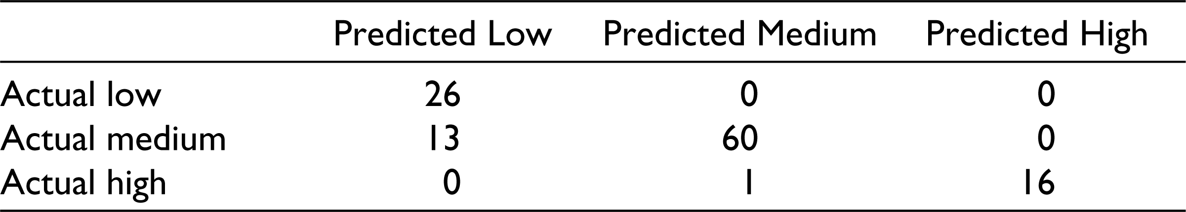
From Table 6, we note that the testing model classifies all banks deemed to be of low health correctly, while it also classifies 60 of the 73 banks deemed to be of medium health correctly. In the case of banks deemed to be in good health, the testing model classifies 16 out of 17 banks correctly. This corresponds to an accuracy of 87.93%.
Additionally, for each pairwise comparison, we calculate the correlation between the discriminant scores and the predictor variables to rank order them in order of relative importance for that comparison. Then, for each predictor variable, the ranks are assigned based on the maximum vote. The result of this analysis is presented in Table 7.
Relative Importance of the Predictor Variables in the Banking Dataset
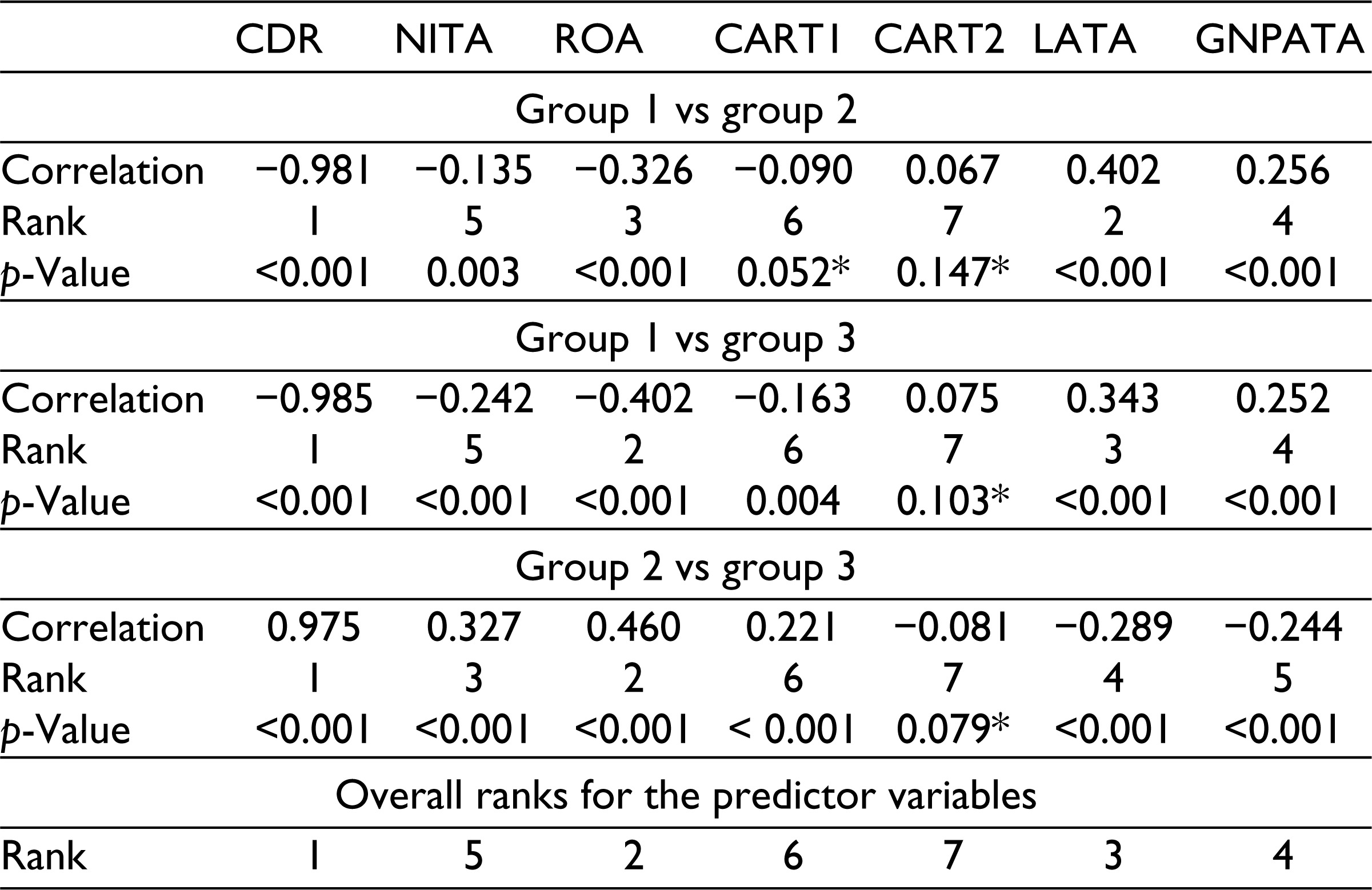
Based on Table 7, CDR is ranked first in all three pairwise comparisons. As a result, it is the most important factor, and hence it gets an overall rank of 1. ROA gets a rank of 2 as it comes second in two pairwise classifications. Similarly, the ranks for GNPATA, NITA, CART1, and CART2 are 4, 5, 6, and 7, respectively. LATA gets a rank of 3 as it has ranks 2, 3, and 4 for the three pairwise comparisons. Further, CART2 was found to be insignificant at the level of significance (a = 0.05) in all three pairwise comparisons, while CART 1 was found to be insignificant at a = 0.05 in the first comparison (group 1 vs group 2). This may indicate that CART2 could be removed as a variable in the classification problem.
Fisher’s discriminant analysis is a popular scoring model used in the classification of two or more groups. With the principal goal of maximizing the separation between the groups, we have developed a spreadsheet model using “Solver” of MS Excel, while avoiding the nuances of computing two-variance-covariance matrices. Further, the two approaches are equivalent when it comes to classification problems with two groups (Morrison, 1976). When it comes to more than two groups, we first perform pairwise comparisons with a common variance, then ensemble the predictions of all pairwise comparisons, and finally take a maximum vote approach for prediction of classes. As a result, we can see that the accuracy of our ensemble approach will be as good as the variance−covariance approach.
We clearly demonstrate the statistical parsimony of LDA with the spirit of Fisher in achieving the largest separation possible between the two groups using two different datasets. LDA seems to have high accuracy over all datasets, and the gist of LDA can be succinctly modelled using the spreadsheet approach.
The spreadsheet modelling approach can be replicated for any discriminant classifier example. We see this as a model that can be easily scaled in terms of records (i.e., even larger datasets can be solved using this approach as the number of constraints is not dependent on the number of records). Note that irrespective of the number of records, there is always one constraint in our optimization model, namely Var (Z) =1.
Additionally, we demonstrate how the results obtained from LDA can be used to rank the predictor variables in order of their importance in the classification problem. This exercise will clearly demonstrate which of the predictor variables are important in the classification problem. Hence, we can use this information to reduce the number of variables in the study. We have shown how this can be accomplished using two datasets from the finance/banking sectors.
Supplemental Material
Supplemental material for this article is available online.
Supplemental Material
Supplemental material for this article is available online.
Supplemental Material
Supplemental material for this article is available online.
Footnotes
Declaration of Conflicting Interests
The authors declared no potential conflicts of interest with respect to the research, authorship, and/or publication of this article.
Funding
The authors received no financial support for the research, authorship, and/or publication of this article.