
Abstract
This article examines the location pattern of unorganised manufacturing enterprises across districts in India. Using a unique data set of 435 districts spread across 25 states, drawn from the Enterprise Survey data of the National Sample Survey (NSS) 1994–95 and 2005–06 ‘thick’ rounds, we find that unorganised manufacturing enterprises are concentrated in a few leading districts, mostly in the metropolitan areas, but their share has declined in the post-reform (post-1991) period, and some new metropolises and suburban districts have emerged as new industrial destinations. The spatial concentration in the distribution of the unorganised manufacturing enterprises across districts has marginally declined—both at the aggregated and disaggregated industry level—in the post-reform period. Our econometric analysis shows that the level of economic development, infrastructure facilities, labour productivity, capital productivity, population size, population density, availability and stock of raw materials, presence and size of organised industries and urbanisation have significant positive effects on the location of unorganised manufacturing enterprises, while economic diversity has a strong negative impact. The specificity of our study is that we use district-level data, which allows us to provide a relatively comprehensive view of the location pattern of unorganised manufacturing enterprises in India.
Keywords
Introduction
One of the major problems faced by the Indian economy in the post-reform period (post 1991) 1 is increasing regional inequality. There is sufficient evidence that inequality has been steadily increasing among states and among regions within states in the post-reform period (Ahluwalia, 2011; Planning Commission, 2013). 2 Researchers have unanimously acknowledged that one of the major causes of aggravating regional (income) inequality in post-reform India is the widening spatial variation in industrial development (Barua & Chakravorty, 2010; Bhattacharya & Sakthivel, 2004; Chakravorty, 2003; Lall & Chakravorty, 2005). Barua and Chakravorty (2010) find that regional inequality in the manufacturing sector is always higher than income inequality levels during 1981–2000 and that manufacturing inequality positively affects regional income inequality. Although there exists a vast literature on the spatial pattern of industrial development in India, most studies are related to the organised manufacturing sector (for example, Alagh, Subrahmanian & Kashyap, 1971; Barua & Chakravorty, 2010; Chakravorty, 2000, 2003; Chakravorty & Lall, 2007; Lall & Chakravorty, 2005; Lall & Mengistae, 2005; Lall, Koo & Chakravorty, 2003; Lall, Shalizi & Deichmann, 2001). Despite the fact that the unorganised manufacturing sector is vast and diverse, and plays important role in India’s industrial sector, few studies have attempted any systematic analysis of the regional aspects of unorganised manufacturing enterprises. 3
In an earlier study (Saikia, 2014), we have analysed the spatial concentration of unorganised manufacturing enterprises in India at two levels—region and state—during 1994–95 to 2005–06. We found widespread inter-regional and inter-state disparity in the distribution of unorganised manufacturing enterprises during the study period. Such disparity, however, is expected in most countries, especially in developing countries like India, given the differences in history, geography, natural resource endowments, stock of human capital, local political economy and culture across the states. Such differences also exist among different regions within a state, which lead to the concentration of economic activities in a few pockets within a state. Even within highly developed states, there are districts which are comparable to the poorest districts in the most backward states (Planning Commission, 2008). Debroy and Bhandari (2003) find that districts with the highest poverty ratios lie not only in backward states like Bihar, Madhya Pradesh, Rajasthan and Uttar Pradesh but also in developed states like Gujarat, Maharashtra, Karnataka and Tamil Nadu. Given such diversity, states as a unit of analysis are large enough, especially in a vast country like India, and hence such an analysis provides only an average picture, which at times is virtually useless, as it cannot capture the trends and patterns at a sub-state level. Therefore, the analysis needs to be extended to a smaller geographical scale, so that variations across regions within a state can be captured. The next largest administrative unit in India is the district. There are about 640 districts as per the 2011 Census. 4 In this article, we extend our analysis to the district level to provide a relatively comprehensive view of the location pattern of unorganised manufacturing enterprises in India and to provide additional guidance for policymakers on targeting their attention.
District-level analysis is a recent trend in India and very few studies have been undertaken to analyse spatial disparities in India at the district level (some examples are Chaudhuri & Gupta, 2009; Debroy & Bhandari, 2003; Singh, Kendall, Jain & Chander, 2010; Topalova, 2005). District-level studies on the spatial pattern of industry in India are even fewer and most of them are focused on the organised manufacturing sector (Chakravorty, 2000, 2003; Chakravorty & Lall, 2007; Lall & Chakravorty, 2005; Sekhar, 1983). One of the early studies (Sekhar, 1983) examined the distribution of industrial employment (both household and non-household industry) among different classes of cities and towns for the period 1960–71 and found that employment in non-household industry was heavily concentrated in Class-I cities, whereas employment in household industries was concentrated in smaller towns. 5 The study further found that during 1961–71, inequality (measured by the Theil index) among the six classes of cities has declined for household industries, whereas it has increased for non-household industry. Chakravorty (2000, 2003) and Chakravorty and Lall (2007) found that spatial concentration (measured by Moran’s-I index) of organised manufacturing industry across Indian districts has increased from 1993–94 to 1997–98. Lall et al. (2001) examined the spatial concentration (measured by spatial Gini index) for 11 organised manufacturing industry groups at the district level for 1994−95 and found that leather products, metal products and food and beverages were the most concentrated industries in India.
Against this background, this article attempts to examine the spatial concentration of unorganised manufacturing enterprises across districts in India from 1994–95 to 2005–06. More specifically, the article has the following objectives:
To analyse the location pattern of unorganised manufacturing enterprises at the district level. To measure the spatial concentration of unorganised manufacturing enterprises across districts. To examine the factors determining the location of unorganised manufacturing enterprises.
We have organised this article into six sections. Following this introduction, Section 2 outlines the data source and Section 3 describes the methodology used in this study. Section 4 analyses the location pattern of unorganised manufacturing enterprises and estimates the degree of spatial concentration of these enterprises across districts at the aggregated and disaggregated industry level. Section 5 examines the factors determining the location of unorganised manufacturing enterprises and Section 6 summarises the findings with policy implications.
Data Source
The main data set of this study comes from the Enterprise Survey data of the 51st (1994–95) and 62nd (2005–06) ‘thick’ rounds of the National Sample Survey (NSS) on unorganised manufacturing enterprises in India. 6 These two rounds of surveys provide enterprise-level information on different characteristics of unorganised manufacturing enterprises in India. 7
Using these data, we have estimated district-level values of the number of enterprises, employment, gross value added and fixed capital. There were approximately 451 districts for 1994–95 and 581 for 2005–06. By employment we mean the total number of employees, which includes both workers and supervisory staff; gross value added is the additional value created by the process of production by an enterprise and is calculated as the difference between ‘total receipts’ and ‘total operating expenses’; and fixed capital is the value of fixed assets owned by the enterprise.
We had to make a number of adjustments for both survey rounds. First, the 51st round provided information according to the four-digit National Industrial Classification (NIC) 1987 codes, while the 62nd round provided information according to the five-digit NIC 2004 codes. Therefore, we reclassified the NIC 1987 codes to NIC 2004 codes at the three-digit NIC level and then aggregated them to arrive at the two-digit NIC 2004 codes. Second, there are some industrial categories which were included in the 51st round but not in the 62nd round, and some industrial categories which were included in the 62nd round but not in the 51st round. Therefore, we have considered only those industrial categories that are covered in both survey rounds.
There were substantial changes in the districts’ boundaries between the two time points because of changes in administrative divisions of the country. Therefore, we constructed consistent district identities by merging the newly created districts with the districts from which they had been carved out, using census atlases and information provided in Kumar and Somanathan (2009). While some districts were cleanly partitioned into multiple districts between these periods, some districts experienced complex boundary changes. In the case of districts that were created by partitioning multiple districts, we use population weights for merging the new districts with the multiple parent districts, following Kumar and Somanathan (2009). Finally, we matched these districts with the NSS district definitions. The number of districts by state considered for analysis is reported in Table 1.
Number of NSS Districts and Districts Available for Analysis
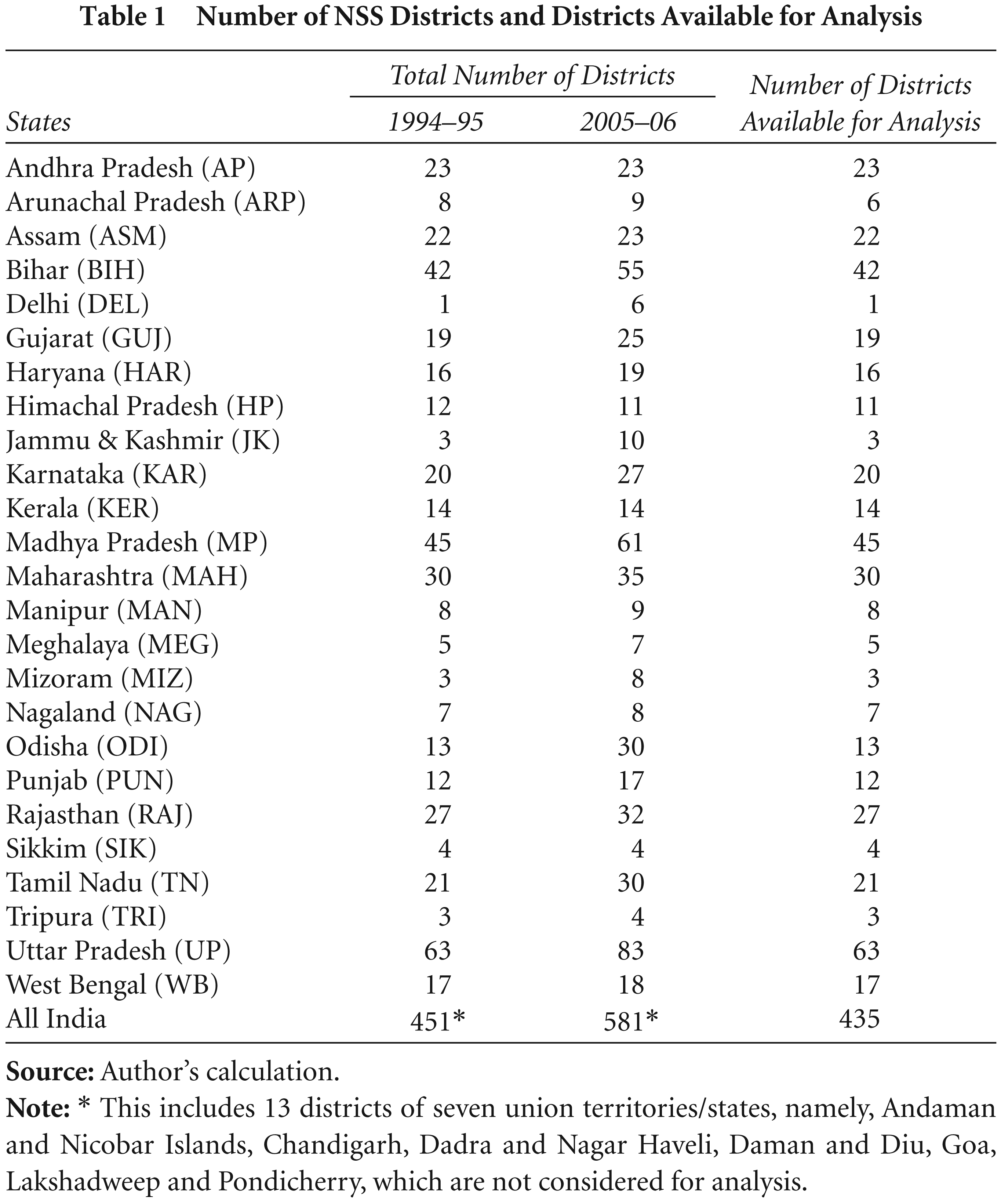
Number of NSS Districts and Districts Available for Analysis
At this stage, a note of caution is worthwhile regarding the district-level estimation of NSS data. There is a common feeling among the scholars that because of the relatively small sample size at the district level (which may sometimes be very small) and the nature of the NSS survey sampling designs, district-level estimates cannot be accurate. Sastry (2003) used the 55th round (1999–2000) of NSS Consumer Expenditure Survey data to estimate district-level poverty ratios and showed that it is feasible to derive valid distributions for a majority of districts on the basis of relative standard errors criteria. 8 Some studies (very few) have used NSS survey data for district-level estimates (for instance, Chaudhuri & Gupta, 2009; Topalova, 2005). 9 Although the reliability of these estimates is not beyond doubt, there is an increasing demand for district-level estimates of important development indicators for main two reasons: the growing divergence among regions within states and the shift in the focus of government policies towards district-level planning. Given the possible error in district-level estimation, one needs to be cautious about the implications of the results drawn upon such estimates.
Data on the other variables were drawn from a variety of sources. The lag values of labour and capital productivity were estimated at the district level by conducting a similar exercise using the Enterprise Survey data of the NSS 56th round (2000–01). District domestic product (sector-wise) for 2005–06 was obtained from the Directorate of Economics and Statistics (DES) of respective state governments. Data on district-level population and geographical area by rural and urban areas were drawn from the 1991 and 2001 censuses (Census of India, Registrar General and Census Commissioner, Government of India). District-wise data on literacy rates, infant mortality rates and percentage of households with access to electricity were drawn from the 2001 census. Data on district-wise number of bank branches were obtained from Branch Bank Statistics, Volume 3 (RBI, 2002) published by the Reserve Bank of India and district-wise road length (for 2002–03) was obtained from Basic Road Statistics, published by Transport Research Wing, Ministry of Road Transport and Highways, Government of India.
The empirical methodology used in this study has three parts. In the first part, we analyse the distribution of unorganised manufacturing enterprises in terms of number of enterprises, employment, value added and fixed capital across 435 districts from 1994–95 to 2005–06 to outline certain emerging features of the location pattern.
In the second part, we employ spatial concentration measures to examine the degree of spatial concentration of unorganised manufacturing enterprises at the district level. We define spatial concentration as the extent to which a given industry is concentrated in a few geographical units (here, districts). Of the various standard measures of spatial concentration proposed in the literature (see Saikia, 2010, for a review of these measures), in this study, we employ two widely used traditional measures, namely, the Herfindahl index and the concentration ratio. The concentration ratio is defined as the percentage share of employment (or output) of an industry located in the largest districts, ranked in descending order. Here, we calculate a four-district concentration ratio. The higher the value of the concentration ratio, the higher will be the degree of spatial concentration.
The Herfindahl index (hereafter the H-index), also known as the Herfindahl–Hirschman index, of an industry, is defined as the sum of squared employment (or output) shares of all districts in the industry. Thus, if Sik is the employment (or output) of the kth district in the ith industry and Si is the employment (or output) of all the districts in the ith industry, then the H-index is defined as

To normalise the effect of the total number of geographical units (n), we compute the normalised H-index (

The value of the H-index ranges from 1 to 1/n (1 = highly concentrated; 1/n = unconcentrated), whereas the value of the normalised H-index ranges from 0 to 1 (1 = highly concentrated; 0 = unconcentrated). An H* value below 0.15 indicates least concentration, between 0.15 and 0.25 indicates moderate concentration and above 0.25 indicates high concentration.
Finally, we perform an econometric analysis to identify the factors that determine the location of unorganised manufacturing enterprises at the district level for the year 2005–06. The model formulation is discussed in the respective section.
Unorganised Manufacturing: Location and Concentration
Location Pattern
Before moving on to analyse the location pattern of unorganised manufacturing enterprises at the district level, we identify certain broad location patterns of these enterprises at the regional and state level (based on Saikia, 2014).
The eastern and central regions emerged as leading regions in terms of employment and gross value added, respectively, during 1994–2005. By 2005–06, the share of eastern and north-western regions had declined, whereas share of southern and central regions had significantly increased.
At the state level, unorganised manufacturing enterprises were concentrated in a few advanced states such as Gujarat, Maharashtra, Tamil Nadu, Delhi and West Bengal during 1994–2005. However, by 2005–06, the share of these states had declined, especially in Delhi and Gujarat, which suffered a drastic decline but continued to be the leading industrialised states.
The industrially backward states are clustered in the northeastern region and the Rajasthan–Odisha belt together with Bihar and Uttar Pradesh, and these states have failed to catch up with the developed states.
In the post-reform period, inter-state concentration has declined for the overall unorganised manufacturing sector and also for many of the two-digit industry groups. In general, high-technology-intensive industries are found to be highly concentrated, whereas resource-based, low-technology-intensive industries are relatively dispersed.
Let us now focus on the distribution of unorganised manufacturing enterprises across districts. Tables 2 and 3 report the shares of the leading districts in the national total in number of enterprises, employment, gross value added and fixed capital for 1994–95 and 2005–06, respectively. 10 These data offer some explanation for the location pattern at the regional and state level summarised above. In the following discussion, we highlight some of the emerging location patterns of unorganised manufacturing enterprises at the district level.
Shares of the Top 20 Districts, 1994–95
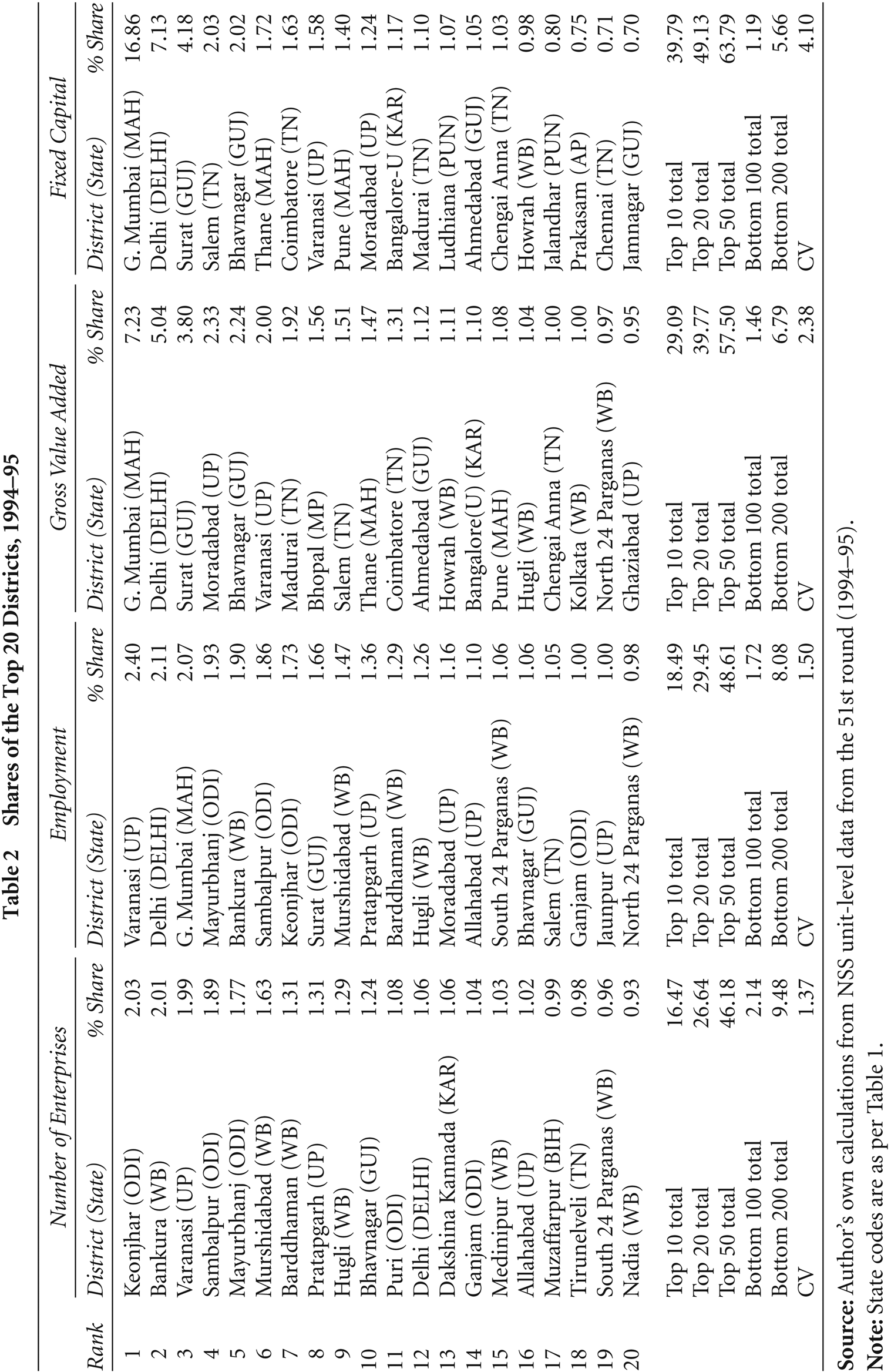
Shares of the Top 20 Districts, 1994–95
Shares of the Top 20 Districts, 2005–06

Decline of leading districts. The shares of the top 10 districts as well as the top 20 and top 50 districts have declined between 1994–95 and 2005–06. Only a few of the top 10 districts in 1994–95 have managed to remain in the top 10 list in 2005–06, 11 but they have all decreased their shares during this period (except for Greater Mumbai and Thane in gross value added and Thane and Coimbatore in fixed capital). The most severe losses were for Delhi, Greater Mumbai and Surat. The decline in the share of Greater Mumbai in fixed capital is greater than Maharashtra’s total loss. Despite this decline, these districts continue to be among the leading industrial districts. At the same time, some of the top 10 districts of 1994–95 have not managed to remain in the top 20 list of 2005–06. 12
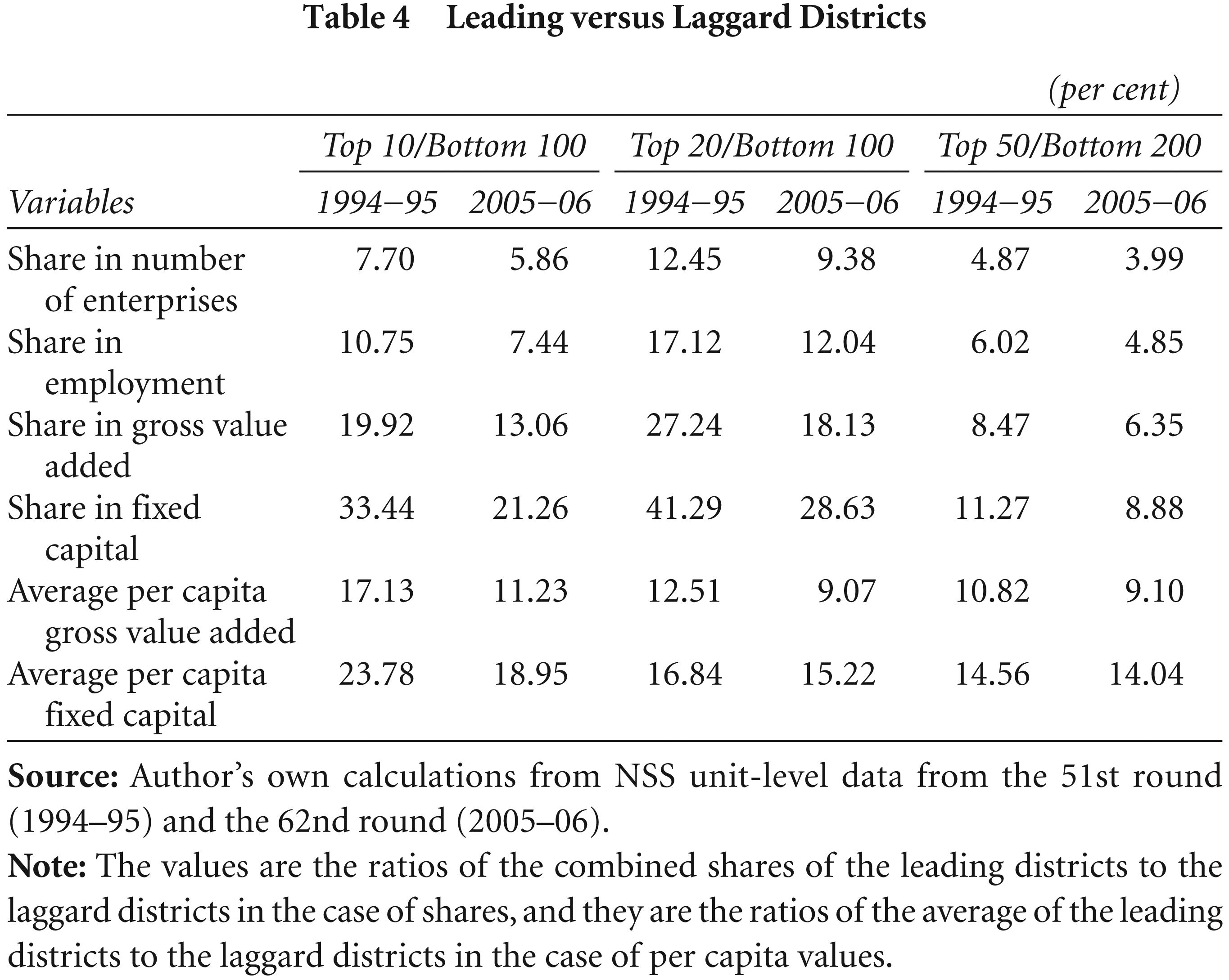
Decline in regional variation. The variation in the distribution of unorganised manufacturing enterprises across districts declined between 1994–95 and 2005–06. This is evident from the fact that the ratio of the share/average of the leading (top 10, 20 and 50) districts to the most backward (bottom 100 and 200) districts has declined during this period (Table 4). This is further confirmed from the decline in the coefficient of variation (CV) across the districts (Tables 2 and 3). However, it is not clear whether or not this decline indicates a convergence pattern in the location of unorganised manufacturing enterprises. The share of the 100 most backward districts has remained almost unchanged and that of the 200 most backward districts has only marginally increased, which means that the most backward districts have failed to catch up with the leading districts. In fact, the decline in spatial variation might possibly be because of the decline of the leading districts only.
Leading versus Laggard Districts
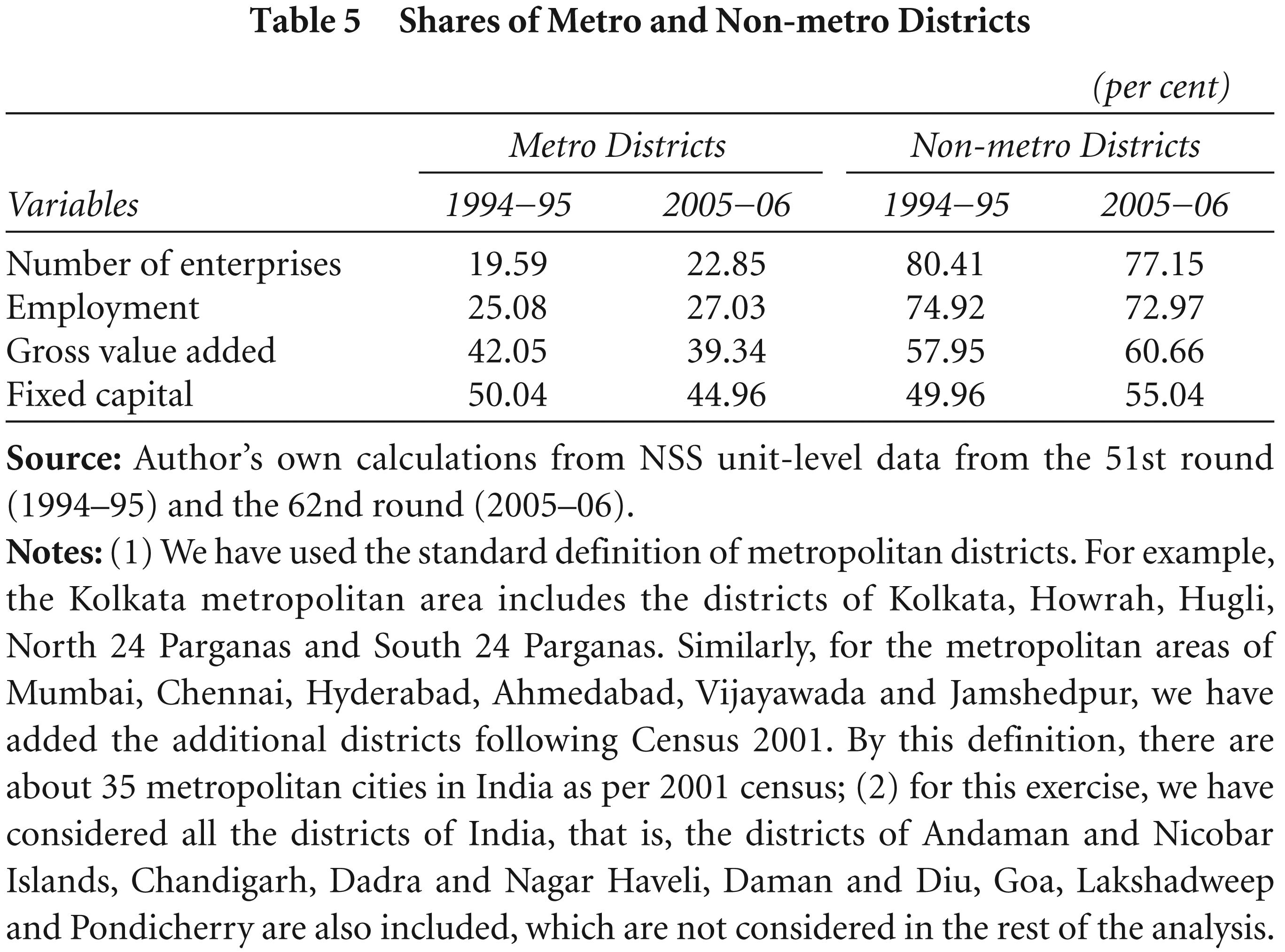
Emergence of new metropolises and suburban districts. Almost all the top 10 districts in terms of gross value added and fixed capital are in metropolitan cities. However, all the metropolitan districts in the 1994–95 top 10 list have lost their shares in 2005–06 (except Greater Mumbai and Thane in gross value added and Thane and Coimbatore in fixed capital) and only a few have managed to occupy a place in the 2005–06 top 10 list (Greater Mumbai, Delhi, Thane, Coimbatore and Surat), while other metropolitan districts such as Ahmedabad, Bangalore, Jaipur, Ernakulum, Meerut and Kolkata have moved to the 2005–06 top 10 list. Overall, the combined share of all metropolitan districts has declined in terms of gross value added and fixed capital (though their shares in number of enterprises and employment have increased, Table 5). 13 This decline is mainly due to the sweeping decline of Greater Mumbai, Delhi, Surat and Varanasi; in fact, ignoring these districts, the combined share of the rest of the metropolitan districts has increased. At the same time, some suburban districts have emerged around the metropolitan areas, for instance, Karimnagar (near Hyderabad), Tiruvanamalai and Vellore (near Chennai), Jalandhar (near Ludhiana and Amritsar), Amreli (near Rajkot), Bhavnagar (near Ahmedabad), Aligarh and Firozabad (near Agra) and Medinipur and Murshidabad (around Kolkata). This suggests that some structural shift has taken place in the location pattern of unorganised manufacturing enterprises across districts in the post-reform period; some industries have spread outward from existing core industrial districts and found new locations in new metropolises and suburban districts.
Shares of Metro and Non-metro Districts
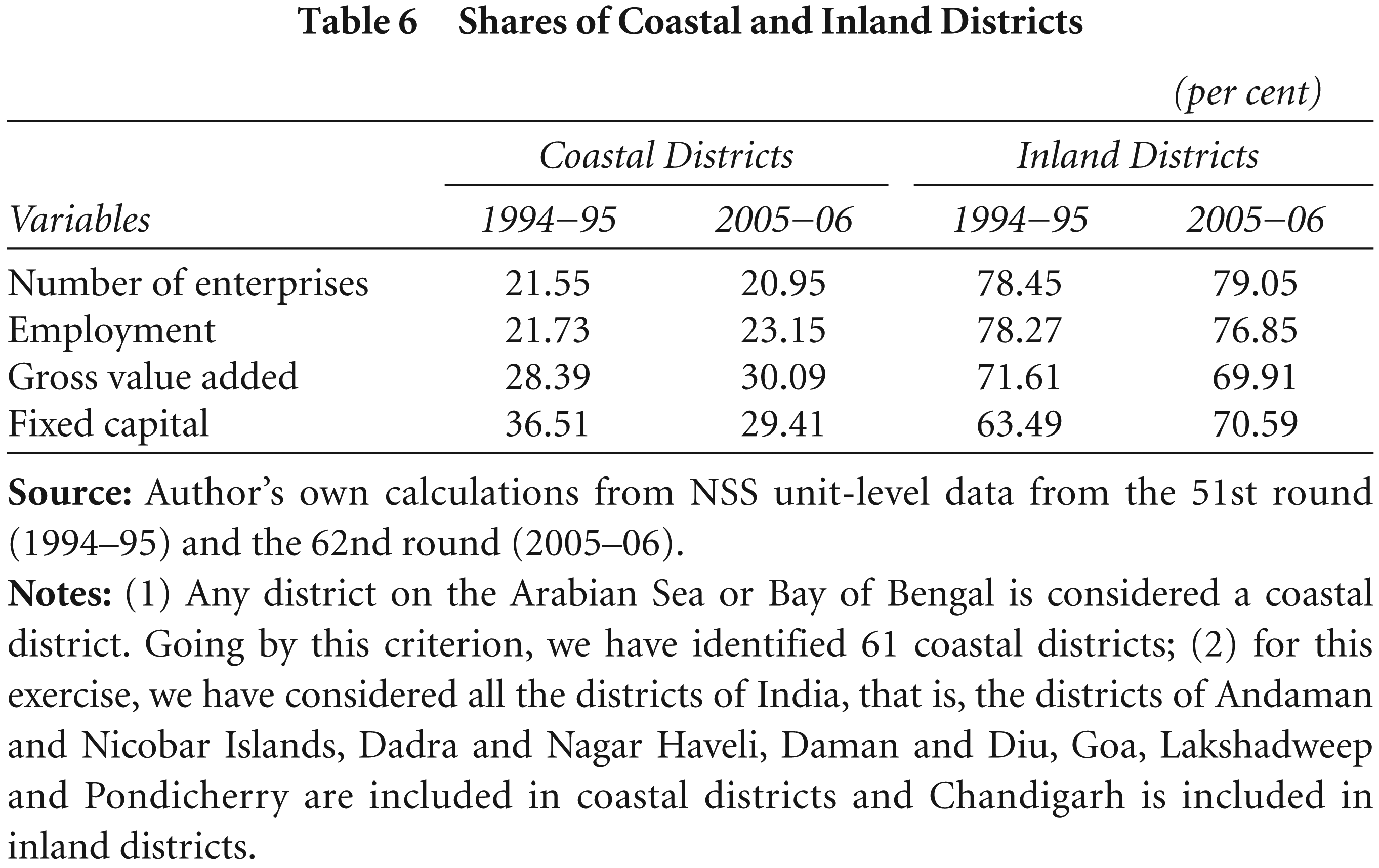
Coastal versus inland concentration. The data presented in Table 6 on the comparative shares of coastal and inland districts reveal that the attractiveness of coastal districts for investment in unorganised manufacturing enterprises has declined (they have lost share in fixed capital), but they have become more productive (gained share in gross value added). There is no evidence for a coastal bias in location of unorganised manufacturing enterprises. The number of costal districts among the leading districts is not different from the number of inland districts.
Clustering of laggard districts. Industrially backward districts are found to be concentrated in backward states such as Bihar, Uttar Pradesh, Madhya Pradesh, Orissa and the northeastern states. 14
Shares of Coastal and Inland Districts
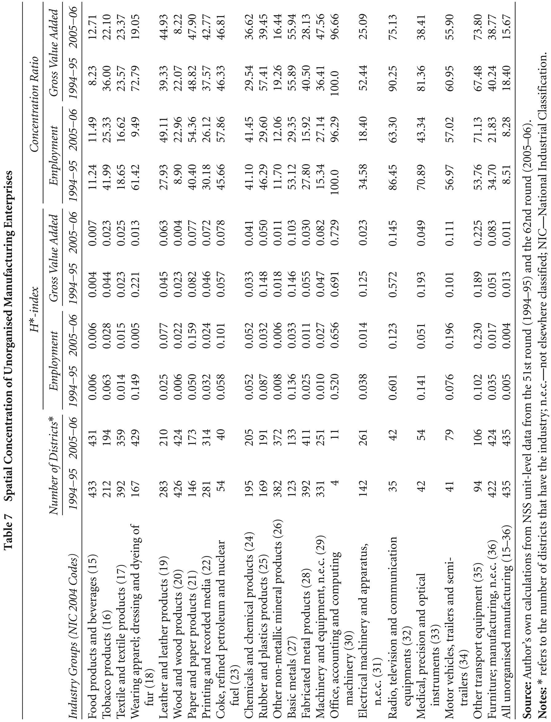
In this section, we examine the spatial concentration of unorganised manufacturing enterprises across 435 districts from 1994–95 to 2005–06. Table 7 reports the results for the normalised H-index and concentration ratio for the aggregate unorganised manufacturing sector as well as 22 two-digit industry groups in terms of employment and gross value added. 15 From the table, it is obvious that manufacturing of office, accounting and computing machinery is the most concentrated industry, being located in only four districts, namely, Greater Mumbai, Pune, Delhi and West Singhbhum, in 1994–95, and no significant spread was observed over a decade. 16 Other industries that show relatively high concentration are: manufacturing of radio, television and communication equipment; medical, precision and optical instruments; motor vehicles, trailers and semi-trailers; and other transport equipment. As against the high concentration of these high- and medium-high technology-intensive industries, the low- and medium-low technology-intensive industries (such as manufacturing of food products and beverages, tobacco products, textile and textile products, leather and leather products, wood and woods products, printing and recorded media, other non-metallic mineral products and fabricated metal products) are the least concentrated industries. 17
Spatial Concentration of Unorganised Manufacturing Enterprises
Spatial Concentration of Unorganised Manufacturing Enterprises
Between 1994–95 and 2005–06, spatial concentration declined for the aggregate unorganised manufacturing sector and for 12 of the two-digit industry groups. Concentration has significantly declined in manufacturing of radio, television and communication equipment; wearing apparel, dressing and dyeing of fur; basic metals; rubber and plastic products and medical, precision and optical instruments. Concentration has increased for manufacturing of office, accounting and computing machinery; motor vehicles, trailers and semi-trailers; other transport equipment; and paper and paper products.
So far, our focus has been on the emerging location pattern and spatial concentration of unorganised manufacturing enterprises across districts. An important question is: what are the factors that determine the location decision of unorganised manufacturing enterprises across the districts? This section aims to find some explanations of the inter-district variation in location of unorganised manufacturing enterprises in India.
The location decision of a firm in a particular region (here, district) depends on a variety of factors. Empirical studies from both developed and developing countries suggest that the most important factors that influence firm’s location decision are: market access, economic diversity, infrastructure facilities, agglomeration economies (localisation economies that arise from intra-industry linkages and urbanisation economies that arise from inter-industry linkages, access to specialised services, a diverse labour market, socio-economic infrastructure, urban amenities, etc.), state policies (fiscal and other incentives; regulations on labour, land, environmental and pollution standards; general level of political support, etc.) and historical forces (Badri, 2007; Chakravorty & Lall, 2007; Deichmann, Lall, Redding & Venables, 2008). In the context of India, recent studies (Chakravorty, 2003; Chakravorty & Lall, 2007; Lall & Chakravorty, 2005; Lall, Koo & Chakravorty, 2003; Lall, Shalizi & Deichmann, 2001) found that economic diversity, clustering of industry in neighbourhood location, availability of labour force and existing industrial concentration play a significant role in determining the location decision of (organised) industries.
Selection of Variables
The literature suggests a long list of factors that influence the location decision of industries, but incorporating all of these in an empirical analysis is not feasible for various reasons (lack of an adequate, reliable database for variables like inter-regional trade, intra-industry and inter-industry linkages, agglomeration economies, etc., and difficulties in quantifying variables such as local entrepreneurship, entrepreneur’s interest, government’s attitude, cultural factors, etc.). This limits the scope of variable selection in our analysis. Therefore, in this study, we explain the location of an unorganised manufacturing enterprise in a district (Ik) in terms of a set of variables representing economic geography (EG), level of economic development (ED), linkages with organised (or large-scale) industries (ORGIND), factor endowments (FREN), infrastructure (INFRA) and spatial attributes of the region (SPAT).
Formally, a model of the following form may be specified:

In our model, Ik represents the presence and size of unorganised manufacturing enterprises in a district and it is expressed in terms of per capita gross value added of unorganised manufacturing enterprises; 18 EG represents a set of three variables: economic diversity, urbanisation economies and market access; ED represents level of economic development and is given by per capita district domestic product; ORGIND represents the presence and size of organised industries; FREN represents a set of three variables: availability and stock of raw materials, labour productivity and capital productivity; INFRA is an index representing four infrastructure variables, namely, physical infrastructure, financial infrastructure, energy infrastructure and social infrastructure, and SPAT represents a set of two dummy variables, namely, coastal and metropolitan. (The definitions and construction of these variables are summarised in Table A.1 in the Appendix.)
Before we proceed it is necessary to explain the effects of these variables on the location decisions of industries, especially unorganised manufacturing industries.
Economic geography has been recognised as the most dominant locational factor by researchers since the development of the New Economic Geography (NEG) theories. The World Development Report 2009 (World Bank, 2009) reiterates the significance of economic geography and argues that the unequal pattern of economic activity and divergence in outcomes across regions are a natural consequence of processes of agglomeration. Researchers have used various elements of economic geography such as market access, transport cost, economic diversity, intra-industry and inter-industry linkages, urbanisation economies and localisation economies. In this study, we use three elements of economic geography: economic diversity, market access and urbanisation economies.
Economic diversity (DIVERSITY) or the industrial mix of a region is an important factor for realising externality benefits arising from inter-industry spillover, heterogeneity of economic activity, increased range of local goods, increased output variety in the local economy and access to better business services such as banking, advertising, and legal services, etc. (Chakravorty & Lall, 2007). Lall et al. (2003) find that economic diversity is the only economic geography variable that has significant cost-reducing benefits for organised manufacturing firms in India and that the effect is higher for small-size firms than the medium- and large-size firms, which implies that small firms can rely on location-based externalities to a larger extent than larger firms. We use the Herfindahl index, as defined in Section 3, to measure economic diversity in each district. Unlike the Herfindahl concentration index that focuses on one industry, the diversity index considers the industry mix of a district. The highest value of Hk is one when the entire district is dominated by one industry. Thus, a higher value implies a lower level of economic diversity. Therefore, we subtract Hk from unity to get a more realistic diversity index, that is, HDVk = 1 – Hk. A higher value of HDVk implies more diversity.
Improved access to market is likely to reduce cost, thereby increasing productivity and demand for a firm’s products, and thus providing incentives to locate closer to the market (Lall et al., 2003). Empirical evidence on the impact of market access on industrial location in India is mixed and depends on the industry type. For instance, Lall and Chakravorty (2005) find evidence for the cost-reducing impact of market access only on metal products and mechanical machinery industries. On the contrary, Lall et al. (2001) find evidence for a positive impact of market access on the leather products and electronics and computer equipment industries, and a negative impact on the non-metallic mineral products and machinery and equipment industries. Thus, the net effect of improved market access need not be always positive. This is because improved market access not only increases demand for a firm’s products and enables investment in cost-saving technologies, thereby increasing profitability, it also increases competition with other domestic firms and with products made internationally, which reduces the monopoly power of firms in the region (Lall et al., 2001).
Access to market is determined by the distance from and the size and density of market centres in the vicinity of the industry. Several different metrics of market access have been used in the literature including market accessibility, distance from transhipment hubs and size and density of market centres. In the absence of reliable district-level data on different distance variables between market centres for construction of a market accessibility index and distance from transhipment hubs, we use market size and density to measure market access. We use total population size (POPSIZE) in the district to measure market size and population density (POPDEN) in the district to measure density of market.
Urban concentration is regarded as an important contributor to economic efficiency, as spatial concentration of economic activity leads to conservation of economic and social infrastructure. The benefits from urbanisation include access to specialised financial and professional services, inter-industry spillovers, economic diversity and availability of general infrastructure such as telecommunications and transportation hubs (Lall et al., 2003). However, these scale economies can be offset by costs such as increase in land rents and wage rates, commuting time for workers, increased transportation costs due to congestion effects and increased competition (Henderson, 2000; Henderson, Shalizi & Venables, 2001). Although there is considerable empirical literature supporting the positive effects of urbanisation economies (Lall et al., 2003), there is little evidence to support the urbanisation economies argument in the Indian context. Lall and Chakravorty (2005) and Lall et al. (2003) find that urbanisation economies either have no benefits or in some instances their magnitude is very small. Lall and Mengistae (2005) find evidence in favour of urbanisation economies only in the technology-oriented industries. On the contrary, Lall et al. (2001) find a significant negative impact of urbanisation on the beverages and tobacco and textiles industries. We use the urban population share (URBPOP) in the district to measure urbanisation economies.
The presence of organised industries is another important factor determining location decision of unorganised enterprises. The presence and size of organised industries encourage the growth of ancillary and subsidiary units. Unorganised enterprises are linked with organised industries through sub-contracting, input–output linkages, market linkages and technological linkages. The linkages between the two sectors can be both forward linkages (through the sale of output, sub-contracting and marketing of products) and backward linkages (via purchase of inputs and raw materials, acquisition of skills and technology, and procurement of credit, etc.). The relationship can be either complementary, where the organised sector helps the growth of unorganised enterprises, or competitive/exploitative, where the organised sector exploits the unorganised sector. In India, by the 1990s, a very substantial part of the unorganised manufacturing sector had developed independent of the organised sector across states (Awasthi, 1991), but in the post-reform period, a fairly sizeable and growing proportion of unorganised manufacturing enterprise is expanding through sub-contracting and ancillary relationships with the organised sector (Bala Subrahmanya, 2004; Sahu, 2007). Available data from the NSS 62nd round show that about 32 per cent of unorganised manufacturing enterprises had sub-contracting relationships with the organised sector in 2005–06. Given the increasing linkages between the unorganised and organised sectors through sub-contracting and ancillary relationships in the post-reform period, we expect that the presence of organised industries in a district will have a positive impact on the location of unorganised enterprises. We measure the presence and size of organised industry in each district in terms of the per capita district domestic product from the organised manufacturing sector (OMPCDDP).
The level of economic development of a district is expected to have a positive impact on the location of industry, because industrialisation progresses with the level of economic development. As Kuznets (1955, 1966) argues, that as per capita income increases, there is a distinct shift in the sectoral allocation towards the industrial sector. Economically advanced regions provide better infrastructure facilities, such as transportation, communication, financial and professional services, accessibility to well-developed factor and product markets and a better business environment, and they are more successful in attracting industries. So, we can postulate that the level of economic development will have a positive effect on industry location. The level of economic development in each district is measured in terms of per capita district domestic product (PCDDP).
The availability of natural resources reflects the potential for growth of resource-based industries. Readily accessible raw materials and their timely availability at lower prices reduce the cost of production, and therefore attract industries. Given that the industrial structure in India and most of the states is dominated by resource-based industries (Alagh et al., 1971; Awasthi, 1991; Papola, Maurya & Jena, 2011; Saikia, 2014; Subrahmanian & Pillai, 1986), 19 the spatial variability of stock of raw materials is likely to have positive effects on industrial location. We measure the stock of raw materials in each district as the per capita district domestic product from agriculture, forestry and logging, fishing and mining and quarrying (AGPCDDP).
Regions that are highly productive attract more industry, since an improvement in productivity helps a firm maximise its profits. A higher level of factor productivity is also a sign of a favourable business environment. We use two factor productivity indicators: labour productivity (LPROD), expressed as the value added per unit of worker, and capital productivity (CPROD), expressed as the value added per unit of fixed capital. The use of these partial productivity measures over total factor productivity, which is a technology indicator, is more appropriate in our view, as unorganised enterprises use very low-level technology and skills. These two variables are measured with a time lag, that is, for year t – 1 (for the year 2000–01, as the NSS conducts a survey on unorganised manufacturing enterprises at five-year intervals) to avoid the probable endogeneity problem. 20
The availability and quality of infrastructure are other important factors in determining industrial location decisions. The positive effects of improved infrastructure facilities and a well-developed transportation network on industrial concentration are well documented in the literature (see, for instance, Chakravorty, 2003; Lall & Chakravorty, 2005; Lall & Mengistae, 2005). The availability of better infrastructure facilities, linking firms to urban market centres, plays important role in minimising the cost of production by reducing transport costs. Further, it increases the probability of technology diffusion through interaction and knowledge spillovers among firms, and the potential for input diversity and, hence, locations with better infrastructure facilities are attractive for location of industries. While one may argue that infrastructure is more important for organised industries than for unorganised enterprises, some infrastructure facilities such as transportation, communication and availability of credit facilities, which are less substitutable by firms, are critical, even for unorganised enterprises. Similarly, the availability of electricity connectivity may be more important for the unorganised enterprises than the organised industries, since having their own power generation systems may be costlier for unorganised enterprises. 21
Data on many infrastructure variables are available at the state level, but there is a scarcity of reliable data at the district level. We have considered four types of infrastructures: physical, financial, energy and social. Physical infrastructure is measured by two variables—road length per 100 sq. km and road length per 100,000 people; financial infrastructure is expressed as the number of commercial bank branches per 100,000 people; energy infrastructure is captured in terms of percentage of households having access to electricity as a source of energy and social infrastructure is measured by two variables—the literacy rate and infant mortality rate. In the analysis, we have constructed an infrastructure index (INFRA) by providing equal weights at each level. The two components of physical infrastructure receive one-half weight each, and so do the two components of social infrastructure. Similarly, the four components of the infrastructure index receive one-fourth weight each. To make the variables comparable, we have normalised them by computing the classic z scores, which is defined as the value of an observed variable minus the variable mean, divided by its standard deviation.
In addition to these explanatory variables, we also include two spatial dummy variables, namely coastal (COASTAL) and metropolitan (METRO) to take into account the locational advantages of coastal and metropolitan regions in attracting industries.
The empirical model employed to estimate the factors determining the location of unorganised manufacturing enterprises at the district level takes the following form:
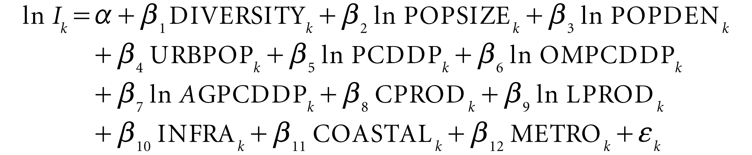
where subscript k denotes the kth district, ln is the natural logarithm, and α, β and εk are interpreted in the usual way. The random error term captures the unobserved characteristics of the location and measurement errors. In the empirical estimation, the signs of the estimated coefficients of DIVERSITY, PCDDP, OMPCDDP, AGPCDDP, CPROD, LRPOD, INFRA, COASTAL and METRO are expected to be positive, whereas that of POPSIZE, POPDEN and URBPOP could be either positive or negative.
We use data for a sample of 399 districts for the year 2005–06 to examine the factors determining the location of unorganised manufacturing enterprises in India. 22 We run the estimation for the aggregate unorganised manufacturing sector as well as for the three enterprise groups: own-account manufacturing enterprises (OAMEs), non-directory manufacturing establishments (NDMEs) and directory manufacturing establishments (DMEs). 23 This allows us to identify which type of enterprise is more impacted by which locational factors. We would hypothesise that the agglomeration forces (such as economic diversity, market access and urbanisation economies) matter less for the OAMEs since these are household-based tiny enterprises and matter more for the DMEs that are modern unorganised enterprises, that is, we expect smaller regression coefficients in the specifications where only OAMEs are included. In the analysis by enterprise types, the number of sample districts has been reduced to 396 in the case of NDMEs and 369 for DMEs, because some districts do not have these enterprises. 24
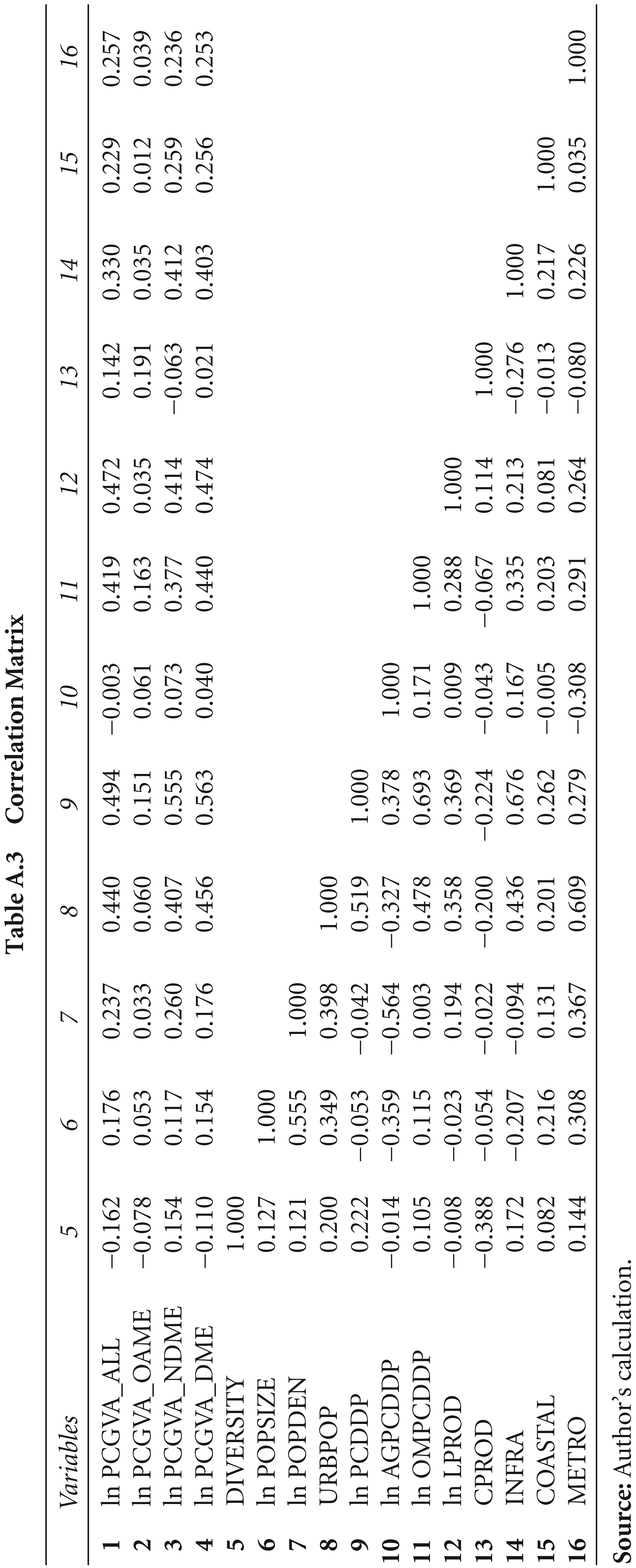
The descriptive statistics of the variables are reported in Table A.2 in the Appendix. We have converted the dependent variable and some of the independent variables to logarithm form, as they were highly skewed in level form. Table A.3 in the Appendix reports the correlation matrix of the explanatory variables, which confirms that there is no high correlation between the explanatory variables, except for URBPOP (with PCDDP, OMPCDDP and INFRA), PCDDP (with OMPCDDP and INFRA) and POPDEN (with POPSIZE and AGPCDDP). Table A.3 also reports the correlation matrix of the dependent variable with the explanatory variables, which reveals that all the explanatory variables, except DIVERSITY, have a positive association with the dependent variable, except for a few exceptions. This confirms the predictions made in the previous section regarding the possible impact of the explanatory variables on industry location, again except for DIVERSITY.
We have employed a double-log form of the ordinary least square (OLS) model to estimate the functional form of industrial location as specified in Equation 2. We have performed the variance inflation factor (VIF) and condition index (CI) tests as suggested by Belsley (1991) to test the presence of multicollinearity; both tests suggested that multicollinearity is not a serious problem. We have also performed the post-estimation test for heteroscedasticity and considered only the corrected estimates along with the heteroscedastic consistent standard error, also known as the robust standard error.
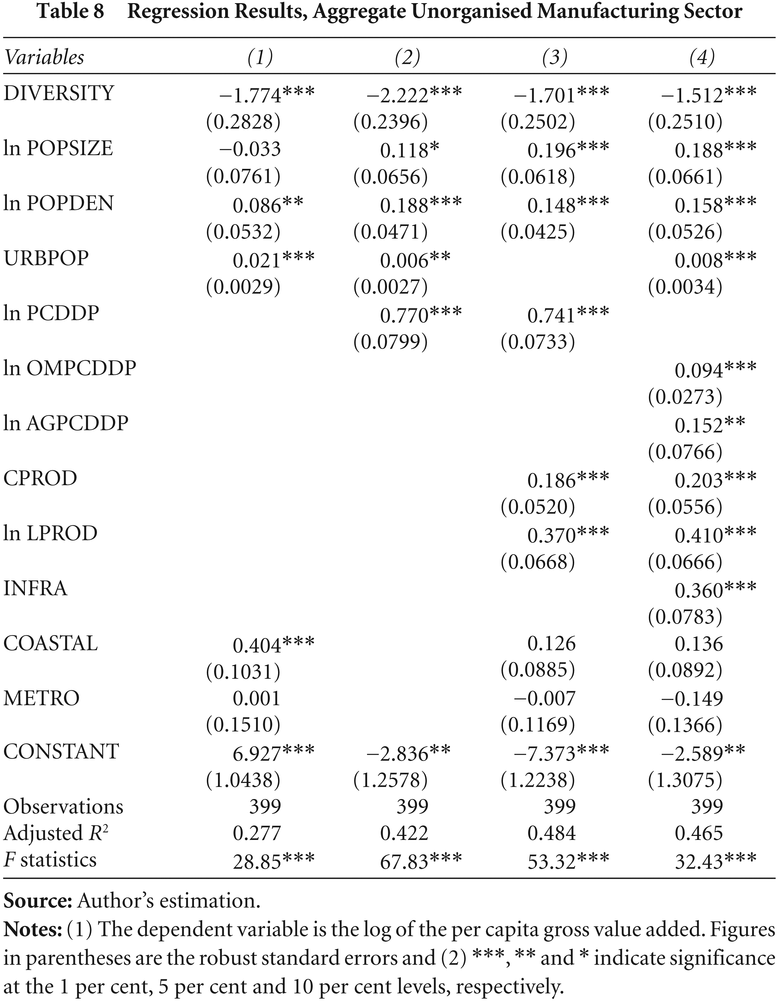
The results of the regression analysis of the aggregate unorganised manufacturing sector are reported in Table 8 and the results for the enterprise types are reported in Table 9. 25 We have performed several iterations with various specifications to tackle the problem of multicollinearity and, finally, considered four specifications with the best possible results (Table 8): (a) agglomeration economies and spatial dummies; (b) agglomeration economies and regional economic development; (c) agglomeration economies plus regional economic development, factor productivity, infrastructure and spatial dummies; and (d) agglomeration economies plus inter-linkages with organised industries, natural resource endowment, factor productivity and spatial dummies. In the case of the enterprise-wise disaggregated analysis, we have reported only the last two specifications, which yield the highest prediction, in order to simplify the tabular presentation. In the following discussion, the results of the two tables are considered together.
Regression Results, Aggregate Unorganised Manufacturing Sector
Regression Results, Aggregate Unorganised Manufacturing Sector
Regression Results, Unorganised Manufacturing by Enterprise Type
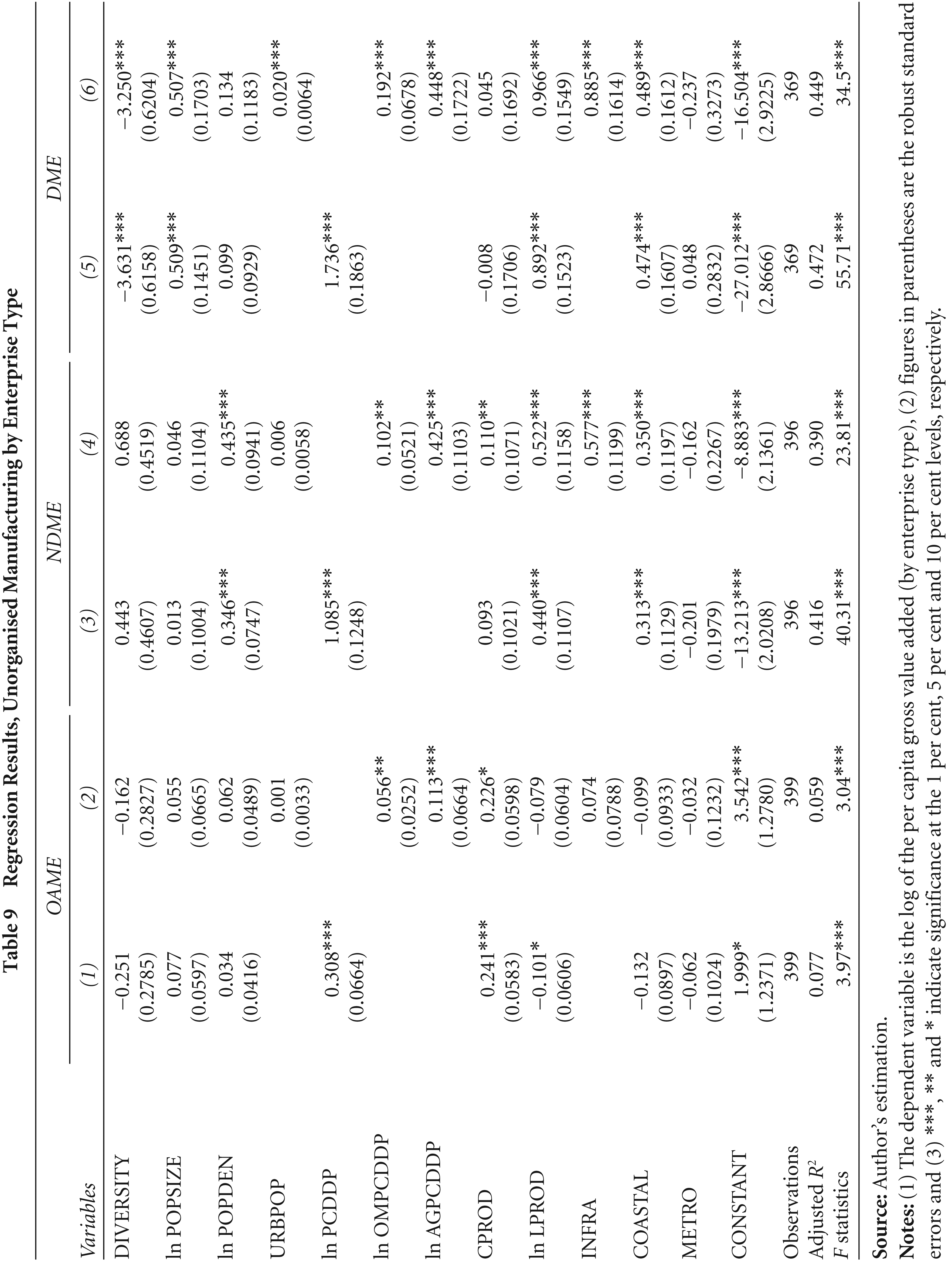
Considering the model sets as a whole, our model explains 27.7–48.4 per cent of the variations in the per capita gross value added of the aggregate unorganised manufacturing sector across districts. The model is less successful in explaining the variations in the per capita gross value added of the OAMEs segment, the adjusted R-square value turns out to be as low as 0.059; but for the NDME and DME segments, the model explains over 39 per cent of the variations in the per capita gross value added.
We first focus on the results for the aggregate unorganised manufacturing sector (Table 8). Regarding the locational effects of the economic geography variables, all three variables are consistently significant. Market access and urbanisation have a positive effect on the location of unorganised manufacturing enterprises; but only market access has a strong influence in determining the size, while urbanisation has little influence. Contrary to our expectation, the effect of economic diversity is negative, which may indicate that the concentration of unorganised enterprises takes place through specialisation in a few industries, while the positive results of other variables suggest the possibility of agglomeration economies.
The variable capturing the level of economic development—per capita district domestic product—turns out to be statistically significant with a positive coefficient sign and strong explanatory power. This suggests that the developed districts attract more enterprises. This may also imply that per capita income, which reflects the purchasing power of buyers and thus the demand for manufactured goods, has a significant impact on the location of unorganised manufacturing enterprises.
The presence and size of organised industries have a positive coefficient sign and are statistically significant. This implies that districts with a large organised industrial sector attract more unorganised enterprises, which further suggests the possibility of the presence of a strong complementary relationship between organised and unorganised enterprises through a sub-contracting and ancillary relationship.
The variables measuring factor and resource endowments—availability and stock of raw materials, labour productivity and capital productivity—are significant and have positive coefficient signs. The positive results suggest that regions that are resource rich and highly productive are preferred for the location of unorganised enterprises, but labour productivity has a strong impact in determining the size of unorganised manufacturing enterprises, compared to availability and stock of raw materials and capital productivity.
As expected, the infrastructure variable, which is measured as an index of the physical, financial, energy and social infrastructure variables, turns out to be statistically significant with a positive coefficient sign and a strong explanatory power.
Finally, of the two spatial dummies, the coastal dummy seems to have a positive effect on the location of unorganised manufacturing enterprises but it is significant only in one specification. On the contrary, the metropolitan dummy is not significant in any of the specifications; in fact, it has a negative sign in two specifications.
These findings are consistent with the existing empirical evidence in the Indian context (Chakravorty, 2003; Chakravorty & Lall, 2007; Lall & Chakravorty, 2005; Lall, Koo & Chakravorty, 2003; Lall, Shalizi & Deichmann, 2001; Mani, Pargal & Huq, 1997, among others), although these evidences relate to organised manufacturing industries at different geographical scales. 26
Now, we focus on the results by enterprise type (Table 9; columns 1–2 report the results for the OAME segment, columns 3–4 report the results for the NDME segment and columns 5–6 report the results for the DME segment). As postulated, all the economic geography variables have virtually no effect on the location of OAMEs and seem to matter only for the DMEs (population density is not significant for DMEs but is significant for the NDMEs). The negative effect of economic diversity can only be confirmed for the DMEs, but in all the specifications, the coefficient has a negative sign. The positive effects of the level of economic development, presence and size of organised industry, and the availability and stock of raw material are confirmed for all three segments of unorganised manufacturing enterprises. However, the effects of factor productivity are found to be inconsistent across the enterprise segments. While the positive impact of capital productivity is confirmed for the OAMEs and NDMEs (in only one specification), to our surprise, it has no significant effect on the location of DMEs (and, in fact, has a negative sign in one specification). Labour productivity has a significant strong positive effect on the location of DMEs and NDMEs, but unexpectedly it has a negative impact on the location of OAMEs. The infrastructure index turns out to be positively significant for DMEs and NDMEs, and also the coastal dummy, whereas the metropolitan dummy is not significant for any of the segments (and has a negative sign across all the sectors). Interestingly, and in line with our expectations, the estimated coefficients of all the variables, except for population density and capital productivity, turned out to be highest in the specifications for the DME segment, which implies that these variables seem to have a greater effect on the location decision and size of DMEs than on NDMEs and OAMEs.
Overall, we find that the location of unorganised manufacturing enterprises is positively affected by the level of economic development, infrastructure facilities, labour productivity, capital productivity, population size, population density, availability and stock of raw materials, presence and size of organised industries, urbanisation and, to some extent, proximity to coastal areas, whereas economic diversity has a strong negative impact. Viewed by enterprise types, the most significant factors having positive effects on the location of OAMEs are: level of economic development, capital productivity, availability and stock of raw materials and the presence and size of organised industries (while labour productivity has a negative effect); factors having positive effects on the location of NDMEs are: the level of economic development, infrastructure facilities, labour productivity, population density, availability and stock of raw materials, proximity to coastal areas, capital productivity and the presence and size of organised industries; and factors having positive effects on the location of DMEs are: the level of economic development, labour productivity, infrastructure facilities, population size, proximity to coastal areas, availability and stock of raw materials, the presence and size of organised industries and urbanisation (while economic diversity has a negative effect).
The critical component of our analysis is that we were unable to identify all the factors that determine the location decisions and size of unorganised manufacturing enterprises in a region. There are several factors related to state- and local-level policies such as subsidies, tax incentives and states’ initiatives to promote industrialisation in backward areas, which play a vital role in attracting new industries into a region. 27 But such factors are difficult to include in an empirical estimation because of the lack of appropriate indicators for such variables and reliable data sources at the district level. Further, in addition to the observed attributes, firms also optimise their location decision based on various unobserved attributes. For example, different regions in India have distinct cultural, political, social and ethnic histories, clearly demarcated linguistic identities and work culture and entrepreneurship habits that have a definite bearing on the attractiveness of a region as an industrial destination. 28 Besides, there are some specific skills inherited by some caste/class/religious groups in certain regions that leads to the formation of industrial clusters based on such skills. 29 But such variables are difficult to quantify and bring into an empirical framework. Last, but not the least, our analysis is only for the aggregate unorganised manufacturing sector and three enterprise types. Location factors may vary from industry to industry, depending on industry-specific characteristics such as inputs used, product categories, technology intensity, and so on, and hence further research is required to account for industry-specific location factors.
The aim of this article has been to analyse the location pattern of unorganised manufacturing enterprises across districts in India and examine the factors determining the location of these industries. Most previous studies on industrial location in India have focused on the organised manufacturing sector at the state level. While focusing on the organised manufacturing sector, these studies have missed out the vast and diverse unorganised manufacturing sector, and by focusing on a state-level analysis, they have missed the broad trends and patterns at the sub-state level. Therefore, this article attempts to cater to the long-felt need to document the location pattern of unorganised manufacturing enterprises across Indian districts, and by doing so, it provides new insights to the existing literature on regional industrial studies in India. The novelty of our study is that we use district-level data, which allow us to provide a relatively comprehensive view of the location pattern of unorganised manufacturing enterprises in India.
The main findings are as follows. First, we find that India’s unorganised manufacturing enterprises are concentrated in a few leading districts, mostly the metropolitan districts. But the share of these leading districts has declined in the post-reform period, mainly due to the sweeping decline in the shares of Greater Mumbai, Delhi and Surat. At the same time, some new metropolises have emerged, such as Ahmedabad, Bangalore, Jaipur, Meerut, Ernakulum and Kolkata, and some suburban districts have also emerged, such as Karimnagar, Tiruvanamalai, Vellore, Bhavnagar, Jalandhar, Amreli, Aligarh, Firozabad, Medinipur and Murshidabad, as new destinations for unorganised manufacturing enterprises in the post-reform period.
Second, spatial concentration in the distribution of the unorganised manufacturing enterprises across districts has declined in the post-reform period. This is evident from the decline in the ratio of the share of leading districts to laggard districts, as well as the spatial concentration measures for the aggregate unorganised manufacturing sector and many of the two-digit industry groups. This decline is due to the decline of the leading districts, while the share of the most backward districts has remained almost unchanged.
Third, our econometric estimations affirm the role of economic geography, regional characteristics and industry-specific characteristics in determining the location decision and size of unorganised manufacturing enterprises. Regarding the effects of economic geography, our findings confirm that it matters only for the DME segment. Overall, the most significant location factors are the level of economic development, infrastructure facilities, labour productivity, capital productivity, population size, population density, availability and stock of raw materials, the presence and size of organised industries and urbanisation; however, economic diversity has a strong negative impact.
The findings have important policy implications. If the policymakers are interested in providing incentives to encourage unorganised manufacturing enterprises to locate in the lagging districts, they need to have an understanding of the relative significance of existing agglomeration forces and local business environment. Our analysis finds that apart from economic geography, local business environment in the form of better infrastructure facilities, high productivity, availability of raw materials and standard of living are the most important factors. Even if there are positive externalities from agglomeration, the local governments could influence the location decisions of unorganised enterprises by offering an impressive array of fiscal and financial incentives.
However, the most crucial factor is the availability of better infrastructure facilities. The poor quality of infrastructure is one of the main reasons behind the economic backwardness of the lagging regions. Unless the basic infrastructure facilities in the lagging districts are improved, mere fiscal and financial incentives will not be able to attract industries to these districts. Therefore, continued public investment is required in backward districts to develop the basic infrastructure facilities such as road and railway connectivity, telecommunication, banking facilities, electricity connectivity, education and health care. Here, the role of the local government becomes important, especially in identifying the key areas that requires the public policy attention most and in providing basic infrastructure to attract new industries. Along with the focus for industrial development in the backward areas, efforts need to be made for technology upgradation, modernisation and sector-specific skill development within the unorganised manufacturing sector, since the sector suffered from low level of productivity. Concrete efforts also need to be made to promote stronger linkages of the unorganised enterprises with agriculture sector and organised manufacturing sector. The national and local governments must take note of these facts while formulating its policies for development of the unorganised manufacturing sector.
Footnotes
Acknowledgements
I am very grateful to Professor K. J. Joseph and Dr Vinoj Abraham for invaluable guidance and support. I also thank an anonymous referee of the journal for helpful comments and suggestions on the article. The usual disclaimer applies.
Appendix
Correlation Matrix
| Variables | 5 | 6 | 7 | 8 | 9 | 10 | 11 | 12 | 13 | 14 | 15 | 16 | |
|
|
ln PCGVA_ALL | −0.162 | 0.176 | 0.237 | 0.440 | 0.494 | −0.003 | 0.419 | 0.472 | 0.142 | 0.330 | 0.229 | 0.257 |
|
|
ln PCGVA_OAME | −0.078 | 0.053 | 0.033 | 0.060 | 0.151 | 0.061 | 0.163 | 0.035 | 0.191 | 0.035 | 0.012 | 0.039 |
|
|
ln PCGVA_NDME | 0.154 | 0.117 | 0.260 | 0.407 | 0.555 | 0.073 | 0.377 | 0.414 | −0.063 | 0.412 | 0.259 | 0.236 |
|
|
ln PCGVA_DME | −0.110 | 0.154 | 0.176 | 0.456 | 0.563 | 0.040 | 0.440 | 0.474 | 0.021 | 0.403 | 0.256 | 0.253 |
|
|
DIVERSITY | 1.000 | |||||||||||
|
|
ln POPSIZE | 0.127 | 1.000 | ||||||||||
|
|
ln POPDEN | 0.121 | 0.555 | 1.000 | |||||||||
|
|
URBPOP | 0.200 | 0.349 | 0.398 | 1.000 | ||||||||
|
|
ln PCDDP | 0.222 | −0.053 | −0.042 | 0.519 | 1.000 | |||||||
|
|
ln AGPCDDP | −0.014 | −0.359 | −0.564 | −0.327 | 0.378 | 1.000 | ||||||
|
|
ln OMPCDDP | 0.105 | 0.115 | 0.003 | 0.478 | 0.693 | 0.171 | 1.000 | |||||
|
|
ln LPROD | −0.008 | −0.023 | 0.194 | 0.358 | 0.369 | 0.009 | 0.288 | 1.000 | ||||
|
|
CPROD | −0.388 | −0.054 | −0.022 | −0.200 | −0.224 | −0.043 | −0.067 | 0.114 | 1.000 | |||
|
|
INFRA | 0.172 | −0.207 | −0.094 | 0.436 | 0.676 | 0.167 | 0.335 | 0.213 | −0.276 | 1.000 | ||
|
|
COASTAL | 0.082 | 0.216 | 0.131 | 0.201 | 0.262 | −0.005 | 0.203 | 0.081 | −0.013 | 0.217 | 1.000 | |
|
|
METRO | 0.144 | 0.308 | 0.367 | 0.609 | 0.279 | −0.308 | 0.291 | 0.264 | −0.080 | 0.226 | 0.035 | 1.000 |