Unilateral Policies,Competitiveness and the ‘Green Paradox’ in a Dynamic North

Abstract

The effects of a unilateral cut in emissions (e.g., by Annexure 1 countries in Kyoto) are analysed in a dynamic two-country two-commodity model. If the fossil fuel is priced at marginal cost, then a unilateral cut reduces total emissions (the carbon leakage is less than 100%). But if the fuel is priced above marginal cost, then a ‘green paradox’ appears, that is, the price of the fuel will fall until its use (over time) exhausts the entire stock. Here, a unilateral policy is self-defeating and it is necessary to get binding commitments on fossil fuel use from all the countries. The production and trade implications for the participant and non-participant countries are analysed.

JEL: Q4, Q50, Q54, Q56

Keywords

Carbon leakage green paradox Hotelling rule quasi-linear preferences

I. Introduction

The total stock of fossil fuel available in the world, if burnt with existing technologies, would add so much to the stock of carbon in the atmosphere that there would be serious consequences for the quality of human life on this planet.¹

1
The stock of carbon in the atmosphere will raise the mean temperature and increase weather variability. The world will see a rise in the sea level (due to a melting of polar ice caps) and a melting of glaciers where some of the big rivers of the world originate. The rise in the sea level will cause migration from the areas that would get inundated, while changes in the weather will require a major change of cropping pattern, etc. Parts of the world would see land becoming more arid. Coping with this would require massive redeployment of resources.

Carbon emissions are a global bad. Climate change is a consequence of the stock of carbon in the atmosphere (as opposed to the flow of emissions). Different nations have contributed to the existing (high) concentration of carbon in the atmosphere in differing amounts. Since carbon is released primarily from industrial activities, the industrialised countries have contributed to the creation of this problem more than the developing economies.²

In the last hundred years, 63 per cent of the cumulative emissions of greenhouse gases have come from the developed economies. Of that, the United States has accounted for 25 per cent and Western Europe for 21 per cent. China and India, home to 40 per cent of the world’s population, have contributed, respectively, 7 per cent and 2 per cent of the last hundred years of cumulative emissions.

(Dutta & Radner, 2012, p. 2)

As the developing countries grow rapidly, their contribution to the stock of greenhouse gases will no longer be negligible. With the existing technologies, if future growth in the developing economies were to be based on burning fossil fuels, then the earth would not be able to cope.³

See Eichner and Pethig (2011), Dutta and Radner (2012) and van der Ploeg and Withagen (2012) for discussions on these issues.

So is there some way that the poorer countries can grow without their growth heating up the planet ‘too much’? Can some alternatives to fossil fuels be subsidised? Or taxes be imposed making the use of fossil fuels more expensive?

The Kyoto Protocol tried to grapple with this twin problem of the heating of the planet and a desire to break out of poverty by the poorer nations by dividing the world into Annexure 1 countries and Annexure 2 countries. The former set had quantitative targets imposed on emissions while the latter did not. In the recently concluded follow-up meeting in Durban, there was a call to include the Annexure 2 countries in the quantitative targets. The meeting also saw Canada (an Annexure 1 country) withdraw from the Kyoto agreement. This article looks at the implications of not including all major economies in restricting global emissions. It focuses on the interaction between the actions of Annexure 2 countries and fossil fuel producers. These are at the heart of including China and India in any future agreement (and possibly, for the withdrawal of Canada).

Thus, we try to answer the question that if a subset of countries become more virtuous (by reducing greenhouse gas emissions), then is it a step in the right direction towards fighting global warming (as was the case in the Kyoto Protocol and the commitment by the European Union to unilaterally cut emissions until 2020)?

Climate negotiations moved away from the Kyoto Protocol to the Paris Agreement wherein each country decides on its contribution (voluntarily) towards a global carbon reduction programme. But with the election of Donald Trump and the withdrawal of the United States from the Paris Agreement, unilateralism is back, except it is the richest country in the world that has removed itself from any binding carbon emission norms! The analysis further goes through with this twist—there are some countries who are not using policies to reduce their emissions. Of course, one has to recognise that the equity principle behind exempting poor countries in the Kyoto Protocol has been replaced by the bullying attitude of the world’s biggest polluter!

International trade and competitiveness issues have been absent from the centre stage of modelling of the climate change economic models, though always lurking in the background of the policy debate (for instance, in Eichner and Pethig, 2011, there is only one final good, so competitiveness issues do not arise). have an intermediate input (oil) and only a single final good). I set up a two-country model—the two countries are identified as Annexure 1 countries (the North) and Annexure 2 countries (the South). North cuts its emissions unilaterally either now or in the future. The model has two goods—called clean or dirty depending on the type of fuel used to produce it. This enables us to analyse terms of trade (or competitiveness) issues that arise from the unilateral policies to mitigate climate change. Finally the model allows for capital accumulation. This is introduced to look at accumulation effects of emission reduction.⁴

It also raises the marginal product of complementary inputs—see Dutta and Radner (2012) for a discussion, although capital accumulation in their model is exogenous.

The answer that emerges to the question whether a unilateral emission cut benefits the world is, it seems, both ‘Yes’ and ‘No’. It depends on the supply curve for fossil fuels. The answer is in the affirmative if the fossil fuel is priced at marginal cost, and the increased demand from, for example, Annexure 2 countries is less than the lower use by Annexure 1 countries (carbon leakage is less than 100%). This is the normal reaction in a market, where following the (exogenous) decrease in the supply of a good, a rise in its price will elicit supplies from other producers—in this case the good in question is a dirty good. The empirical evidence based on CGE models (see, e.g., Burniaux & Martins, 2000; IPCC, 2007) estimate carbon leakages to be about 20 per cent, at most.

The pessimistic ‘No’ comes from a concept known as ‘the green paradox’⁵

The concept is due to Hans Werner Sinn (2008). It has spawned a large literature, most of it in a partial equilibrium setting. See for example (in addition to the references in the text) Gerlagh (2011) and Hoel (2010).

that has attracted the attention of practitioners in the area of environment and resource economics. This paradox occurs if the price of fossil fuel (that initially exceeds marginal cost) collapses following a decline in its demand as the world tries to grapple with global warming. Think of this as the decision by governments to, for example, subsidise a ‘clean fuel’ (say wind, solar, etc.). The fall in the price of fossil fuel may well result in an increase in emissions (certainly in some periods and in those economies where the clean fuel is not subsidised). To see this, note that with the price of the fossil fuel set above marginal, then it would be increasing at the rate of interest (a la Hotelling). Suppose the exhaustion of the fuel stock was to occur at date T. Now suppose the oil producers expect that at T’<T, oil would be replaced by a clean fuel. If the marginal cost of extraction is zero (thus all revenue is rent), then the oil producers would pump out all the oil by T’. Assuming the interest rate remains unchanged, this means a lower price on all dates between now at T’. Thus, oil demand would be stimulated during this period, unless the clean technology is cheaper than this path (bounded further by the marginal cost of production).

The problem of global warming (i.e., the aggregate effects) has two dimensions. The first is the level of emissions. These have to reduce drastically because the initial stock in the atmosphere is very large. The second is the timing: given a level, postponing emissions is better, that is, emission cuts have to be front-loaded. The green paradox may violate both of these.⁶

See van der Ploeg and Withagen (2015) for an elaboration of the term green paradox—different authors use different welfare measures. For our purposes, since we are not doing a welfare analysis, the discussion in the text would do.

It leaves the overall level of fossil fuels unchanged and may (but not necessarily so) bring higher emissions forward in time. This possibility implies that the South, that would be the font of carbon leakage cum green paradox, has to be roped in to be part of the climate agreement. Also, the analysis points towards the use of quantitative restrictions of emissions in the absence of (possibly) time-varying optimal taxes.⁷

The green paradox is based on the reaction of producers to the decline in the price of fossil fuel when subsidies to clean fuel or taxes on the fossil fuel are set at arbitrary (as opposed to optimal) levels—see Hoel (2010) for a discussion of the nature of those taxes. One can possibly appeal to (even in the absence of uncertainty) Weitzman’s quantitative restriction argument because the effects of the green paradox occurring would be catastrophic.

There is by now a large literature that deals with these issues. A number of papers have looked at the logical consistency of the green paradox in partial equilibrium settings. The outcome is mixed. In a general equilibrium setting, there are papers by van der Ploeg and Withagen (2010, 2011, 2012), Eichner and Pethig (2011) and Smulders, Tsur, and Zemel (2010). Van der Ploeg and Withagen (2011, 2012) and Smulders et al. (2010) look at a closed economy infinite horizon optimal growth model where two sources of energy—a clean backstop and a fossil fuel are perfect substitutes.⁸

In Smulders et al. (2010), there is a sunk cost of using the clean fuel.

The closed economy models, while very illuminating, still leave a lot to be desired. The poorer economy is not a replica of a rich economy in the past, both existing in autarky.⁹

This is reminiscent of the convergence literature in growth theory, where, for example, China or India may have a lower output per capita given their lower capital–labour ratios compared to the United States. No trade is allowed. If we open up these economies to trade, within a Heckscher–Ohlin set-up, factor-price equalisation would ensure that there is no convergence—both economies via their Euler equations would have identical growth rates of consumption (see Chen, 1992).

In the real world, the rich and the poor trade with one another, climate change negotiations typically focus on the competitive advantage that might accrue to those economies that are allowed to pursue lax environmental policies.

The three major exceptions to the closed economy modelling are di Maria and van der Werf (2008), Eichner and Pethig (2011) and Sen (2016). The former looks at trade and directed technical change, but without the intertemporal element in fossil fuel pricing. They find that there is carbon leakage when a subset of countries embarks on limiting fossil fuel use, and that this is reduced by directed technical change. Eichner and Pethig (2011) set up a two-period model (with one final good produced with fossil fuel being the variable input) to analyse carbon leakages and the green paradox.¹⁰

A three-period model is also discussed as an extension.

It, by choice, abstracts from trade in final goods and capital accumulation that are the focus of the current article. In Sen’s (2016) two-period model, no equalisation of interest rates takes place.

There have also been some interesting papers analysing technical change to make growth ‘cleaner’. Some of these take into account the nature of the fuel market, in particular exhaustibility and the endogenous response of resource owners (see, e.g., Chakravorty, Leach, & Moreaux, 2011; Grafton, Kompas, & van Long, 2010; Henriet, 2012, albeit in a partial equilibrium setting). Others like di Maria and van der Werf (2008) and Acemoglu, Aghion, Bursztyn, and Hemous (2012) look at directed technical change but do not discuss this in any detail.¹¹

In the two papers closest to ours, di Maria and van der Werf (2008) look at carbon leakage but not the dynamic nature of fossil fuel pricing; while Eichner and Pethig (2011) have only one final good and no capital accumulation. Since they also do not allow for borrowing or lending, their intertemporal substitution parameter is redundant. In equilibrium, countries consume the production of their final good output. For an analysis of borrowing and lending and the effect of carbon leakage on the world interest rate, see Sen (2012).

It is true that we could have a disastrous change in climate even without exhaustibility of fossil fuel. But for some fuels exhaustibility is the endogenous optimal response of the suppliers. In this case (the green paradox), these authors could be seriously underestimating the magnitude of the environmental problem.

Finally, there is a strand of the literature that emphasises strategic interaction (see, e.g., Barrett, 2003; Chatterji, Ghoshal, Walsh, & Whalley, 2011; Finus, 2001). Dutta and Radner (2012) analyse the strategic interaction with capital accumulation (being treated as exogenous—more like disembodied technical progress).¹²

Their conclusion about ‘aid’ from the rich to the poor countries to make the latter participate in cutting back emissions is similar to the policy implications obtained in this article. I focus on different issues, though.

This article should be seen as providing a slightly different perspective on the use of different types of fossil fuels. Van der Ploeg and Withagen (2012) have drawn our attention to the fact that oil (and gas) is less polluting than coal, and hence should be used exclusively initially. My analysis suggests that while this may be true, oil is much more likely to upset the applecart of climate change negotiations because of the presence of Hotelling rents.

What about the distribution of welfare losses (in a more general set-up ‘competitive’ advantage) between the belt-tightening Annexure 1 countries and the ‘free-riding’ Annexure 2 countries. This requires two goods to analyse a terms of trade advantage. As mentioned earlier in Eichner and Pethig (2011), for instance, there is only one final good and thus there is autarky in ‘value-added’.

Before turning to my model, I also note that the analysis further has implications for free trade in goods (import of fossil fuel embodied in goods). As the production of the dirty good moves to those countries that do not cut fossil fuel use, those who do can continue to import these by exporting the clean good. Thus, in the context of the recent climate change negotiations, how much of the increased Chinese emissions should actually be debited to the American account, since they will consume the goods produced? I do not pursue this line of enquiry as it would take us too far afield (see Whalley, 2011, for a discussion on trade and environment negotiations).

II. The Model

Consider a three-period model. Not much happens in the third period in which the fossil fuel input is not available, having either been exhausted or been prohibited by policy or superseded by innovation—this is the equivalent of the ultimate clean steady state of van der Ploeg and Withagen (2011). Two goods—called clean and dirty—are produced and consumed in each country initially. International borrowing or lending is not considered and thus trade is balanced in each period. The first period is one where the capital stock is given by history, the second and the third period capital stocks are optimally chosen. The fossil fuel producers are not considered separately as a third bloc (as do Eichner & Pethig, 2011). If they are, then imagine that only the value-added in each economy is available for consumption and capital accumulation, and that the fossil fuel producers consume the dirty good only. Unlike Copeland and Taylor (2005), there is no trade in pollution permits. Emissions between blocs remain strategic substitutes. No strategic interaction between the bloc of countries is considered (as in Barrett, 2003; Dutta & Radner, 2012; Finus, 2001), nor defection or entry into blocs (unlike Babiker, 2005). It will become clear that free-riding pays, but in the presence of the green paradox this comes at the expense of everyone becoming worse off.

As discussed in the Introduction, the first period is one where the accumulated carbon in the atmosphere is likely to make life in the future difficult. Thus, policy should endeavour to reduce carbon emissions as much as possible. Also, too much emission now could exacerbate the problem. So given the total emissions, postponing these is desirable.

Consumers

The representative individual in each country has a utility function defined over the three periods with a constant discount factor given by β. There are two goods, indexed ‘X’ (the numeraire) and ‘Y’. The instantaneous utility function is quasi-linear.¹³

13
See Bond, Iwasa, and Nishimura (2011) for a discussion of non-homothetic preferences in dynamic trade models.

The utility function is linear in the clean good X.¹⁴

Quasi-linearity makes the utility derived from dirty goods concave but the utility from the clean good is linear.

For the North then we have:

U \equiv C_{^{1}} + β C_{^{2}} + {(β)}^{2} C_{^{3}}

(1)

C_{^{i}} \equiv {\tilde{x}}_{^{i}} + u ({\tilde{y}}_{^{i}}) ​ i = 1, 2, 3.

(2)

For the South, we have identical preferences¹⁵

Preferences are identical but not homothetic.

U^{*} \equiv C_{1}^{*} + β C_{2}^{*} + {(β)}^{2} C_{3}^{*}

(3)

In the earlier equations, a subscript (t = 1, 2, 3) denotes the time period, and the South’s corresponding variables are denoted by an asterisk. In principle, the rates of time preference could be different but to keep the analysis simple let us assume that they are identical. This will enable us further, given quasi-linearity, to talk of ‘the’ rate of interest in any period.

Note, given the public bad nature of global warming, we do not explicitly mention this as an argument in the utility function. It is easy to incorporate a term in each period to take cognizance of the stock of greenhouse gases, for example, Π1 = Π0 + π1, where Π0 is the stock of emission at the beginning of period 1 and π1 is the emission in period 1 (net of any regenerative capacity of the environment).

The Firms

Let us turn to production decision by firms. A firm solves a static problem in each period. It is assumed to rent the capital from households and choose the allocation of capital between the two ‘sectors’ as well how much of the clean and fossil fuels to be used (the specific factors are, naturally, not mobile between sector and earn rents). The dynamic part of the firms’ problem is delegated elsewhere—the household decide on investment and the fossil fuel suppliers decide on the time path of the price of fuels. First, I present the static decisions of the firm.

The clean good (its supply denoted by X) is produced using capital (KX), clean energy, S, that is supplied (perfectly elastically) at a price s, and some specific factors (ZX).¹⁶

The clean energy could be inelastically supplied, but then it would be indistinguishable from ZX. The main results of the article do not depend on the supply curve for S.

The dirty good (whose supply is denoted by Y) is produced using capital (KY), fossil fuel (R) supplied at a price q and some specific factors (ZY). The Zi’s are inelastically supplied. The framework of production is that one of specific factors and thus capital is instantaneously mobile between sectors (though not internationally or across periods).¹⁷

Our analysis imposes quantitative restrictions on fossil fuel use (as do Eichner & Pethig, 2011). Ishikawa and Kiyono (2006) look at non-equivalence of various types of emission-reducing policies. It is possible to include an abatement technology but it does not seem worth the additional complications.

Carbon emissions are proportional to the use of fossil fuel worldwide. The production allocation in any period in the North is represented by (time subscripts will be introduced later).

ℜ (1, p, K, q, s; Z^{X}, Z^{Y}) = \max_{K^{X}, K^{Y}, R} {F (K^{X}, S, Z^{X}) + p G (K^{Y}, R, Z^{Y});_{}^{} K = K^{X} + K^{Y}}

(4)

The production functions F(.) and G(.) are increasing and linearly homogeneous in their respective three arguments, with diminishing marginal productivity. Since the Zⁱ’s are fixed, the two production functions are strictly concave in the variable inputs KX, and S, and KY and R, respectively. It is noteworthy that armed with quasi-linearity and the strict concavity of the production functions in their variable inputs, all the signs of the comparative static effects further are determined unambiguously!

The revenue function involves equating the value of marginal product of capital in the two sectors (5a), the marginal product of the clean fuel to its price (5b), and the marginal product of the fossil fuel input equal to its market price (5c).

F_{K} (.) = p G_{K} (.)

(5a)

F_{S} (.) = s

(5b)

p G_{R} = q

(5c)

A similar set of equations describe the production block in the South.

Market-clearing

In the absence of international borrowing and lending, trade is balanced between the two countries. The two goods are traded in the first two periods (in the third, only one good is produced in either country so there is autarky). Market-clearing requires, in any period, Equation (6) to hold—the left-hand side is the total supply of the dirty good and the right-hand side is the total demand:

ℜ_{p} (.) + ℜ_{p}^{*} (.) = \tilde{y} + {\tilde{y}}^{*}

(6)

By Walras’ law, the market for the clean good also clears (shown in Equation (7) to highlight that capital accumulation involves the clean good) (note the subscript 1 here is the constant price of the clean good and not a time subscript):

ℜ_{1} (.) + ℜ_{1}^{*} (.) = (\tilde{x} + I) + (\tilde{x} * + I *)

(7)

In the light of the interest rate being constant¹⁸

.Note that it is the product interest rate in terms of the X-good that is constant, and not the consumption interest rate.

in the model (see further), agents in each country decide on

\tilde{x} + I

and allocate between these two heads via the constant interest rate.

Further, we shall see that the South will expand its dirty good production, when the North imposes restrictions on the use of fossil fuel (we will let the North and the South be identical in their endowments and hence there is no reason to trade in the absence of, for example, different attitudes to fossil fuel use). In Eichner and Pethig’s (2011) one final good model, such a restriction makes the North’s (their ‘Abating Countries’) GDP and consumption fall one-for-one. In my model, The North’s consumption of the dirty good need not fall, even when its production does.

Dynamics

There are three sources of dynamics in this model, two of them familiar from optimal growth models, namely the investment and the consequent accumulation of capital, and allocation of consumption across periods via the Euler equation (or the Keynes–Ramsey rule). The third comes from models of natural resources—when we have the Hotelling rule in the pricing of the fossil fuel.

Investment in any period becomes next period’s capital stock (implicitly assuming 100% depreciation).¹⁹

Nothing hinges on this. Assuming zero depreciation makes no difference to the analysis. A rate of depreciation that lies between zero and one would necessitate carrying the parameter of depreciation in calculating the expected marginal product of capital.

So,

I_{t} = K_{t + 1}

(8)

In a dynamic context, the linearity of the utility function in good X ties down the real rate of interest (in terms of good X) to be equal to the rate of time preference.

(1 + r) β = 1

(9a)

(1 + r^{*}) β * = 1

(9b)

If the discount factors are identical, as is assumed here, then r = r^*.

Finally, the demand for fossil fuel across periods must be at most equal to the existing stock. The demand for fossil fuels occurs in the first two periods when the dirty good is produced:

\bar{R} \geq R_{^{1}} + R_{^{2}} + R {}_{1}^{*}+ R_{2}^{*}

(10)

If Equation (10) holds as an equality, the price of fossil fuel must satisfy the Hotelling rule (since fossil fuel reserves can be extracted in either period).²⁰

We assume a constant marginal cost of extraction, c. If the cost of extraction were variable (e.g., stock-dependent, then the Hotelling rule would hold for one unit—all units with lower cost of extraction would be mined now, all units with a higher cost would be mined in the future. This is clear by setting different c’s in Equation (11).

q_{t + 1} - c = β^{- 1} (q_{t} - c)

(11)

In Equation (11), the left-hand side is the surplus from extracting one unit of the fuel in the next period (with c being the constant marginal cost of extraction), while the right-hand side represents the surplus today carried over to tomorrow at the interest factor β-1.

This implies

β q_{t + 1} = q_{t} + (β - 1) c

(12)

On the other hand, if demand is strictly less than the exogenous stock of the fossil fuel (in Equation (10)), Equation (11) holds trivially with

q_{t + 1} = q_{t} = c

(13)

That is, marginal cost pricing prevails.

Of course, policy and climate change negotiations are precisely in place to ensure that Equation (10) does not hold with an equality—all or some of the terms on the right hand are sought to be reduced. Note, as emphasised by Acemoglu et al. (2012), that an environmental disaster is possible even when the natural resource is not exhaustible. We consider the exhaustible case also because it comes with a sting in its tail (i.e., the ‘green paradox’).

This completes the description of the model. Let us collect the equations describing the model to be used in Table 1, before turning to the analysis of the problem at hand.

Equations T1.1 and T1.2 are the market-clearing equations for the clean good in period 3.

Equations T1.3 and T1.4 (T1.7 and T1.8) are the equality of marginal products of capital to the real interest rates in the two sectors in the North (South) in period 2. Equation T1.5 (T1.9) is the equality of the marginal product of the clean fuel to its exogenous price, s, in the North (South). Equation T1.10 is the equality of the marginal product of fossil fuel to its price in the South (recall this may not be true for the North—T1.6). Finally, Equation T1.11 is the market-clearing equation for the dirty good.

Table 1.

Summary of the Model with Marginal Cost Pricing

Period 3
$F (K_{3}^{X}, S_{3}, Z^{X}) = {\tilde{x}}_{3}$	T1.1
$F (K_{3}^{X }, S_{3}^{}, Z^{X }) = {\tilde{x}}_{3}^{}$	T1.2
Period 2
$F_{K} (K_{2}^{X}, S_{2}, Z^{X}) = β^{- 1} = p_{2} G_{K} (K_{2}^{Y}, R_{2}, Z^{Y})$	T1.3, T1.4
$F_{S} (K_{2}^{X}, S_{2}, Z^{X}) = s$	T1.5
$p_{2} G_{R} (K_{2}^{Y}, R_{2}, Z^{Y}) \geq q_{2}$	T1.6
$F_{K} (K_{2}^{X }, S_{2}^{}, Z^{X }) = β^{- 1} = p_{2} G_{K} (K_{2}^{Y }, R_{2}^{}, Z^{Y })$	T1.7, T1.8
$F_{S} (K_{2}^{X }, S_{2}^{}, Z^{X *}) = s$	T1.9
$p_{2} G_{R} (K_{2}^{Y }, R_{2}^{}, Z^{Y *}) = q_{2}$	T1.10
$G (K_{2}^{Y}, R_{2}, Z^{Y}) + G (K_{2}^{Y }, R_{2}^{}, Z^{Y }) = \tilde{y} (p_{2}) + {\tilde{y}}^{} (p_{2})$	T1.11
$K_{2}^{X} + K_{2}^{Y} = K_{2}$	T1.12
$K_{2}^{X } + K_{2}^{Y } = K_{2}^{*}$	T1.13
Period 1
$F_{K} (K_{1}^{X}, S_{1}, Z^{X}) = p_{1} G_{K} ({\bar{K}}_{1} - K_{1}^{X}, R_{1}, Z^{Y})$	T1.14
$F_{S} (K_{1}^{X}, S_{1}, Z^{X}) = s$	T1.15
$p_{1} G_{R} ({\bar{K}}_{1} - K_{1}^{X}, R_{1}, Z^{X}) \geq q_{1}$	T1.16
$F_{K} (K_{1}^{X }, S_{1}^{}, Z^{X }) = p_{1} G_{K} ({\bar{K}}_{1}^{} - K_{1}^{X }, R_{1}^{}, Z^{Y *})$	T1.17
$F_{S} (K_{1}^{X }, S_{1}^{}, Z^{X *}) = s$	T1.18
$p_{1} G_{R} ({\bar{K}}_{1}^{} - K_{1}^{X }, R_{1}^{}, Z^{Y }) = q_{1}$	T1.19
$G ({\bar{K}}_{1} - K_{1}^{X}, R_{1}, Z^{Y}) + G ({\bar{K}}_{1}^{} - K_{1}^{X }, R_{1}^{}, Z^{Y }) = \tilde{y} (p_{1}) + {\tilde{y}}^{*} (p_{1})$	T1.20
Fossil Fuel
$R_{1} (q_{1}) + R_{1}^{} (q_{1}) + R_{2} (q_{2}) + R_{2}^{} (q_{2}) \leq \bar{R}$	T1.21
$β q_{2} = q_{1} + (β - 1) c$	T1.22

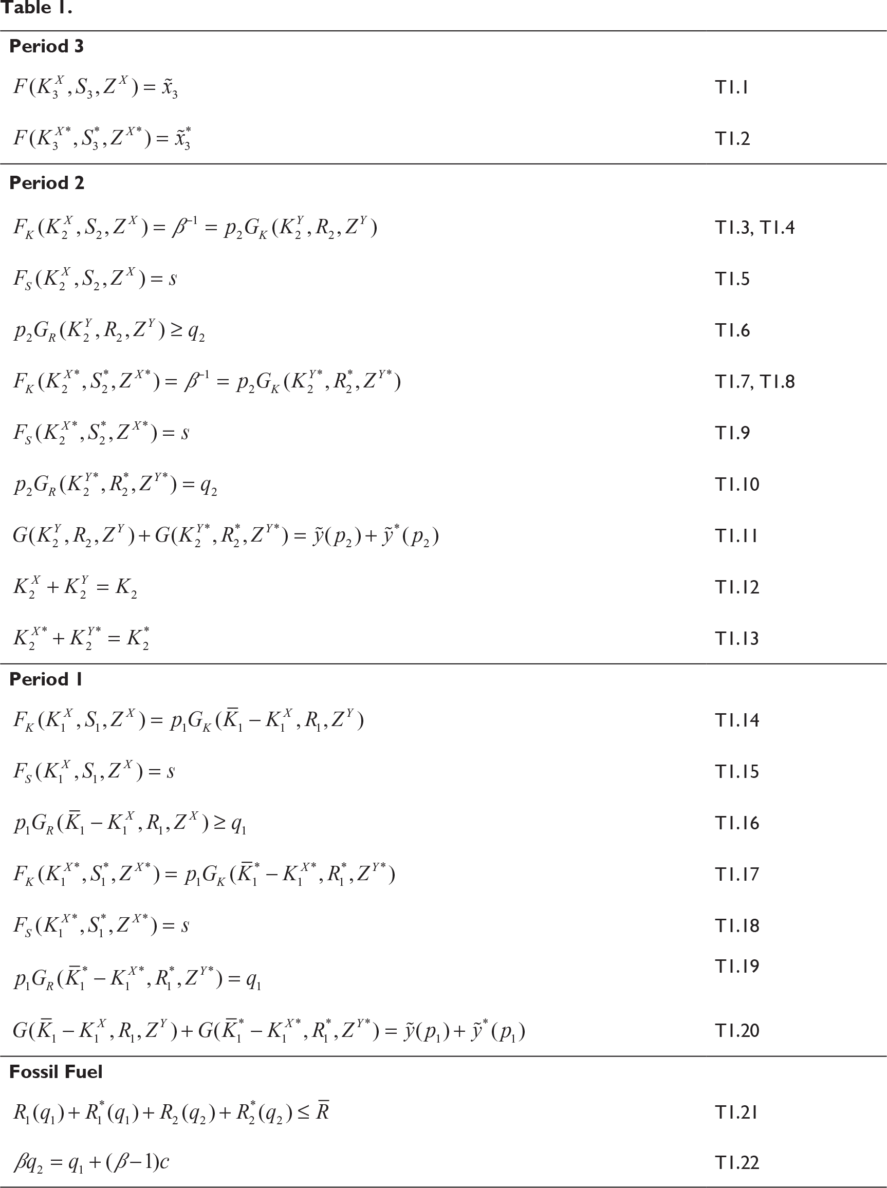
A similar interpretation is to be used for period 1 (T1.14 to T1.20) except that now the initial capital stock is historically given and, while there is mobility of capital between sectors to ensure the equality of marginal products, the return to capitals is no longer tied to a given real interest rate.

To anticipate (and avoid repeating) some tedious derivation further, note that for period 2, Equations T1.4, T1.6 (with an equality), T1.8, T1.10 and T1.11 can be solved for $K_{2}^{Y}, R_{2}, K_{2}^{Y *}, R_{2}^{*}$ and $p_{2}$ in terms of $q_{2}$ . When T1.6 does not hold with an equality, the other four equations can be solved for and $p_{2}$ , in terms of $q_{2}$ and some specified level of $R_{2} (= {\bar{R}}_{2})$ . Note that the X sector inputs do not impinge on the Y sector, because capital (in either sector) for period 2 is chosen such that its marginal product equals β-1. Equations T1.3 and T1.5 determine the unique values of $K_{2}^{X}$ and $S_{2}$ . Similarly, Equations T1.7 and T1.9 determine the values of $K_{2}^{X *}$ and $S_{2}^{*}$ .

For period 1, Equations T1.14 to T1.20 (when T1.16 holds as an equality) can be solved for $K_{1}^{X}, S_{1}, R_{1}, K_{1}^{X *}, S_{1}^{*}, R_{1}^{*}$ and $p_{1}$ , in terms of $q_{1}$ . But when T1.16 does not hold with an equality, the other six equations can be solved for $K_{1}^{X}, S_{1}, K_{1}^{X *}, S_{1}^{*}, R_{1}^{*}$ and $p_{1}$ in terms of $q_{1}$ , and some specified level of $R_{1} (= {\bar{R}}_{1})$ .

Let us now turn to the effects of a unilateral cut in fossil fuel use by the North. In Section III, fossil fuel is supplied competitively with marginal cost pricing, while in Section IV there is an endogenous mark-up over marginal cost and the Hotelling rule kicks in.

III. Restriction on Fossil Fuel Use in the North: Marginal Cost Pricing

Before turning to the analysis of effects of a restriction on fossil fuel use by the North, let us define a few terms.

Definition 1: Carbon leakage is the increase in emissions by the South in any period relative to the cut in the North’s fossil fuel use (in that period).

Definition 2: A green paradox occurs if the total emission across the two periods stays unchanged, after a reduction in fossil fuel use by the North in either period.²¹

21
Note that this is different from the way some others use this term, for example, Eichner and Pethig (2011). They use this term to imply 100 per cent or more leakage within the same period. It is also different from the definition(s) given by Gerlagh (2011).

We shall see later in this section that carbon leakage by our definition (without the green paradox) turns out to be less than unity (in absolute value). Taken together, these definitions imply that when the green paradox occurs some, leakage necessarily spills over to periods without a cut in fossil fuel use (the carbon leakage in these periods would be infinity).

We start off with the case of marginal cost pricing of the fossil fuel. While this maybe empirically relevant for some fossil fuels, for example coal, it also serves to prepare us for the Hotelling rule case discussed in the next section.²²

Eichner and Pethig (2011) do not discuss marginal cost pricing of the fossil fuel—in their analysis the marginal cost is zero.

Marginal cost pricing implies that the supply curve for fossil fuels is horizontal, and, given a constant marginal cost, supply is demand-determined.

We look at two specific situations: Either (a) in period 1 the North will reduce its production of the dirty good or (b) it will do so in period 2—this is anticipated in period 1²³

Complete cessation of production of the dirty good in the North is a simple extension in the framework of this article. It, however is not a ‘small’ change and is imperfectly served by calculus.

Period 1

R_{1} (c) + R_{1}^{*} (c) + R_{2} (c) + R_{2}^{*} (c) 〈 \bar{R}

Suppose now the North restricts the fossil fuel input at some exogenous level ${\bar{R}}_{1}$ , where its marginal product exceeds the market price. The quotas are auctioned and the revenue rebated to the households in a lump-sum fashion. Qualitatively, we would obtain similar results if we allowed for taxes on fossil fuel use, rather than quantitative control on its use.

When T1.16 does not hold with an equality, that is,

p_{1} G_{R} ({\bar{K}}_{1} - K_{1}^{X}, {\bar{R}}_{1}, Z^{Y}) > q_{1} (= c),

we solve the six equations (T1.14, T1.15 and T1.17 to T1.20) for $K_{1}^{X}, S_{1}, K_{1}^{X *}, S_{1}^{*}, R_{1}^{*}$ and $p_{1}$ in terms of $q_{1}$ (= c here), and some specified level of $R_{1} (= {\bar{R}}_{1})$ —the appendix provides the details. To get some intuition on what happens, we first solve, Equations T1.14, T1.15 and T1.17 to T1.19 for $K_{1}^{X}, S_{1}, K_{1}^{X *}, S_{1}^{*}$ and $R_{1}^{*}$ in terms of $p_{1}$ and ${\bar{R}}_{1}$ . We then substitute these values in the market-clearing condition T1.20 to obtain a value of $p_{1}$ in terms of ${\bar{R}}_{1}$ . That equation gives the excess demand for the Y good caused by the reduced supply due to the restriction on fossil fuel use by the North, and the necessary increase into eliminate it. We then substitute this back in T1.19 to obtain a value for $R_{1}^{*}$ in terms of ${\bar{R}}_{1}$ .

What does this tell us about fossil fuel use in the ‘non-abating’ countries? We would expect some carbon leakage as fossil fuel demand in the abating countries falls. Although its price is tightly tied to the marginal cost of production (and therefore does not change), its demand in the non-abating South increases via an excess demand for the dirty good that manifests itself in a rise in $p_{1}$ . How much of the decreased demand for fossil fuels in the North is made up by for increased demand in the South? Is it possible that it is more than 100 per cent?

The answer is that the excess demand for the dirty good is met partly through increased production (using more fossil fuel), and partly through an increase in price of the good. This is what one would expect in a well-behaved market with Walrasian price adjustment. More than 100 per cent increase in the use of fossil fuel (apart from a lacking in good economic intuition) would make an increase in fossil fuel use by the North a policy to (partially) mitigate climate change—this would no doubt be music to the ears of the oil lobbies and climate-change-deniers!

In our set-up we have (again see the appendix for details),

- 1 < d R_{1}^{*} / d {\bar{R}}_{1} = - {G_{R} (\partial R_{1}^{*} / \partial p_{1})} {[- β (\partial K_{1}^{X} / \partial p_{1}) - β (\partial K_{1}^{X *} / \partial p_{1}) + G_{R} (\partial R_{1}^{*} / \partial p_{1}) - (\tilde{y}' (p_{1}) + {\tilde{y}}^{*}' (p_{1}))]}^{- 1} < 0

(14)

The denominator in Equation (14) is the excess demand for the dirty good and the numerator is only a fraction of that. The fact that the derivative is negative implies that the oil use are strategic substitutes across the two blocs.²⁴

See the discussion on strategic complimentarity versus strategic substitutability in Copeland and Taylor (2005).

And that it is less than minus one implies that the carbon leakage is less than 100 per cent—the exact magnitudes depending on the other terms that figure in the denominator.

Period 2

Imagine that there is marginal cost pricing, but now a (foreseen in period 1), reduction in fossil fuel use in the North in period 2, such that the marginal product of fossil fuel exceeds its price, that is,

p_{2} G_{R} (K_{2}^{Y}, {\bar{R}}_{2}, Z^{Y}) > q_{1} (= c)

Again the quotas are auctioned and the revenue rebated to the households in a lump-sum fashion.

We can solve the four Equations T1.4, T1.8, T1.10 and T1.11 for $K_{2}^{X *}, K_{2}^{Y *}, R_{2}^{*}$ and $p_{2}$ in terms of ${\bar{R}}_{2}$ (see the appendix for details).²⁵

As earlier, we shall first solve for the seven variables in terms of $p_{2}$ and ${\bar{R}}_{2}$ Then solve for in terms $p_{2}$ of ${\bar{R}}_{2}$ Finally multiply the resultant expression by to obtain Matters are helped enormously by the fact that unlike period 1,anddo not vary with ${\bar{R}}_{2}$ .

The carbon leakage is again less than 100 per cent (Equation 15):

- 1 < d R_{2}^{*} / d {\bar{R}}_{2} = - {c (\partial R_{2}^{*} / \partial p_{2})} {[β (\partial K_{2} / \partial p_{2}) + β (\partial K_{2}^{*} / \partial p_{2}) + c (\partial R_{2}^{*} / \partial p_{2}) - (\tilde{y}' (p_{2}) + {\tilde{y}}^{*}' (p_{2}))]}^{- 1} < 0

(15)

The interpretation is the same as that for a period 1 reduction, with one major difference: when in period 1 the North reduces its use of fossil fuel, capital is relocated from the Y-sector to the X-sector. Its Y-output falls compared to the laissez-faire level but there is increased production of X. In period 2, on the other hand, the output of the X sector is given by the input use determined solely by Equations T1.3 and T1.5 (and therefore do not change).²⁶

For the South, similarly, Equations T1.7 and T1.9 uniquely determine input use in the clean sector, and hence the size of that sector.

In other words, North’s GDP falls one-for-one as a consequence of the reduction in the dirty good production.

Imposing control on fossil fuel use in both periods by the North results in the sum of the effects in the individual periods and needs no further elaboration.²⁷

Quasi-linearity is important here. We do not have to worry about capital accumulation being affected when the restriction on fossil fuel is operative in both periods.

Proposition 1: When the Hotelling rents are zero, a cut in emission by a subset of countries increases emissions by the other countries in that period. This resultant increase is, however, less than the initial cutback. Thus, there is carbon leakage but less than 100 per cent. There is no effect of this policy in the other period(s).

Remark: The non-participant (free-riding) countries benefit from an increase in their GDP as their Y-sector output expands and also from a reduction in global emissions (a slower growth in the stock pollutant in the atmosphere).

A simple extension gives us Proposition 2:

Proposition 2: Reduction of fossil fuel use in both the periods is the sum of the single period effects. Hence carbon leakage lies (in absolute value) between zero and one.

(IV). Positive Hotelling Rents

Period 1 Emission Cut

What happens to worldwide use of the fossil fuel if the North cuts its use of these in the first period, in the presence of positive rents in the price of fossil fuel? The market price of fossil fuel follows the Hotelling rule (Equation 16), with the price in both periods exceeding marginal cost. The scarcity rents arise from limited fuel supply over the two periods being equated to the demand for it (Equation T1.21 holding as an equality).

β q_{2} = q_{1} + (β - 1) c,_{}^{} q_{1}, q_{2} > c

(16)

R_{1} (q_{1}) + R_{1}^{*} (q_{1}) + R_{2} (q_{2}) + R_{2}^{*} (q_{2}) = \bar{R}

(17)

The exposition of this section is helped enormously if we recognise the analysis of the previous section is the effect of the stricter abatement policy in the North with the price of fossil fuel held constant (of course, in contrast to the previous section, in this section the price is above marginal cost). The only additional bit required in the analysis is to allow the q_i’s to adjust so that Equations (16) and (17) hold. To anticipate the detailed results further, we saw that in Section III, compared to the initial situation, there was an excess supply of fossil fuel after the adjustment (with price of fossil fuel constant). Now if its price were allowed to adjust it would decline in that period but not so much that takes its (fossil fuel) demand back to the initial equilibrium. The quantity demanded in the period that the policy is implemented, must be less than initial demand, that is, carbon leakage in that period is not 100 per cent. The reason why this is so, is that if the price of fossil fuel falls today, it must also fall tomorrow (and vice versa) via the Hotelling rule.²⁸

.In my model, the real product interest rate is pinned down by the rate of time preference. It is possible that in other models, where this is not the case, fossil fuel prices across periods are not so tightly linked. See for example Strand (2010) for a detailed discussion of the interest rate.

If carbon leakage is 100 per cent today, then there will be excess demand for fuel in the other period (and hence over the two periods). Thus, carbon leakage will continue to be less than 100 per cent in this period (more generally, in the year of the abatement policy), but will be infinity in the next period (in the year that the abatement policy is not in place).²⁹

.In these years, the reduced emission due to abatement is zero (and this is in the denominator for calculating carbon leakage in any period).

We also know (either from the set of Equations T1.3 to T1.13, or from the set T1.14 to T1.20) that fossil fuel use is negatively related to its price in any period when there is no voluntary restriction, that is,

d R_{t} / d q_{t} = (\partial R_{t} / \partial q_{t}) + (\partial R_{t} / \partial p_{t}) (d p_{t} / d q_{t}) < 0

(18)

(This is a statement that the own price effect is always negative.)

In the first case, the North reduces fossil fuel use in period 1. Since in the first period, capital stocks are given by history, as capital in the North is shifted to the clean good, its rate of return will fall. As capital shifts to the Y-sector in the South, its production of clean goods would fall, but the rate of return to capital will rise. The price of fossil fuel falls in both periods, causing production of the dirty good to rise in the South in both periods, as well as in the North in the second period. Since the size of the clean sector in either country remains unchanged in period 2, there will be an investment boom in period 1 worldwide.

Proposition 3: If the North reduces its fossil fuel use in period 1 with positive Hotelling rents, the dirty industry expands in the South in both the periods, while it expands in the second period in the North (after contracting initially). Fossil fuel use across the two periods is unchanged but there is less use of it in period 1.

Comment: This is akin to the EU going it alone now to combat climate change with the possibility that it would reverse its position in the absence of a global agreement (or many Canadas defecting from the Kyoto Protocol in the future). While it does precious little to combat overall emissions, it does change the time profile of emissions away from the present.

Period 2

If the price of the fossil fuel falls, now consider the additional effects (to those in Section III) in period 2. Capital accumulation in period 1 in the North would fall in the dirty sector—so that the marginal product of capital in that sector stays unchanged (fossil fuel is Edgeworth-complimentary with capital—if less of it is used, the marginal product of capital falls). The marginal product of capital schedule in the South will shift out in the Y-sector as the price of fossil fuel falls, while remaining unchanged in the clean sector. In the first period, its capital accumulation will be speeded up. In period 2, the world will produce the same amount of clean goods and a lower amount of the dirty good (because of diminishing marginal productivity the price of the dirty good also rises).

Since the price of oil has to rise at the rate of interest (the Hotelling rule), there will be first period effects also. The price of fossil fuel would be lower in the first period and both North and South will witness an expansion in the dirty sector. Pollution in period 1 definitely rises in this case, while period 2 pollution falls (since the sum total of world fossil fuel is given).

To sum up, dirty goods production is relocated spatially and intertemporally. Period 2 witnesses a slowdown in activity. The clean good output continues to be the same, but the total production of dirty goods falls. In period 1 dirty goods production increases, because fossil fuel is cheaper now and clean goods output falls globally, as capital is relocated to the dirty sector.

If cleaning up one’s act implies reducing fossil fuel use, we are not getting anywhere. The South uses all the fossil fuel that the North does not. This is also inefficient (in a production sense) because of diminishing returns to capital. And dirty goods production is brought forward in time.³⁰

In Indian English, it is called ‘preponing’, in symmetry with ‘postponing’.

Proposition 4: If the North reduces its fossil fuel use in period 2 with positive Hotelling rents, the dirty industry expands in the South in both the periods, while it expands in the first period in the North (while contracting in period 2). Fossil fuel use across the two periods is unchanged but there is more use in period 1—an unmitigated environmental disaster.

The pattern of trade is quite clear. In the periods that the North reduces its use of the fossil fuel, it would import this good from the South and pay for this by restricting its demand for the clean good below its production levels (note that in period 2, the production of the clean good is unchanged globally after the restriction on the use of fossil fuel).

Now, in passing, consider the case where the North makes binding commitments in both periods. In this case, there may not be any relocation of production across periods, although there is spatial relocation in both periods. Think of a knife-edge case. Due to the reduced demand in the two periods from the North, fossil fuel prices fall and in each period the increased demand for it in the South just matches the reduced demand in the North. Worldwide production efficiency goes down, without any change in either total emission or its distribution over time. Of course, dirty production is relocated to the South.

But this is just a knife-edge case. If the use of the fossil fuel changes across periods then, depending on the details, it is possible that carbon leakage in one period exceeds 100 per cent, matched by an equivalent shortfall in the other period, since the sum total of emissions across the two periods is unchanged.

The upshot of all this is that it is imperative that the South’s demand for fossil fuels be curtailed. A quantitative target for dirty goods production could be imposed. An equivalent tax could be imposed—this would be rising over time, as the South accumulates capital. Or the world could do the ‘mother of all sequestrations’ by making a transfer to the fossil fuel producers to keep their valuable resource underground (geological sequestration).

In a trading world, country-wise production-based emissions make no sense. Emissions have to be consumption-based. Some of China’s recent increase in emissions should be attributed to the US consumption.

V. Conclusions

I have outlined a model that highlights the reaction of the market economy to a reduction in carbon emissions. The analysis in the literature so far has concentrated on carbon leakages—a movement along a given supply curve for fossil fuels. The problem is compounded by the green paradox, that is, a shift down of the supply curve. Fossil fuel producers have an incentive to reduce their prices, as long as it is above marginal cost, and to bring forward the time profile of extraction. This would benefit those countries which do not have binding emission commitments (e.g., India and China, as has happened in Durban recently). Trade would take some of this dirty production back to the now ‘clean economies’. It is therefore imperative that developing economies with large industrial bases be brought within the ambit of climate change agreements with strict binding constraints. In the presence of the green paradox, it is even more ironical that those economies that did not create the problem (of the stock pollutant) have necessarily to be part of the solution. But the emerging economies may well ask ‘What is it in this for us?’ Thus, serious side payments, technology transfers, etc. have to be considered.

The model needs extensions. The quasi-linear utility fixes the interest rate—this is useful as an expository device but surely lacking in realism. No international borrowing or lending is considered here. The extraction of oil is possible at constant marginal cost. The backstop is available in infinite supply at a given price. All these need modifications. In an open economy context, whether pollution is caused by production or consumption is important—though in a global bad context it is less important (since the world is a closed economy).

Finally, the issue of many fossil fuels, some whose supply is elastic (e.g., coal), and others (e.g., oil) whose known sources involve pricing above marginal cost, needs careful analysis. The latter class involves exploration for new sources, and that is elastic in supply. At any point in time, however, with large sunk and fixed costs, the price of the output of existing oil wells exceed marginal cost. Thus, a serious attempt at combating climate change would involve elements of both Sections III and IV.

Acknowledgements

Some of the material was presented in invited lectures at conferences in Exeter and the Singapore Economic Review Conference, and at seminars in Oxford and Toulouse. I am grateful to Jean-Pierre Amigues, Michael Finus, Peter Lloyd, Michel Moreau, Francois Salanie, Tony Venables and Alan Woodland for helpful comments. Special thanks to Rick van der Ploeg and Roger Guesnerie for extensive discussions. Also to Brian Copeland, who persuaded me to reduce my exposition from an infinite horizon model to a three-period one. Finally, thanks are also due to an anonymous referee of this journal for his/her interesting comments on an earlier version of this article. The usual disclaimer, however, applies.

Declaration of Conflicting Interests

The author declared no potential conflicts of interest with respect to the research, authorship and/or publication of this article.

Funding

The author received no financial support for the research, authorship and/or publication of this article.

A. Appendix

Emission Tightening in Period 1 (Marginal Cost Pricing)

Home Country

Emission control in the North means $G_{K} (K - K_{1}^{X}, {\bar{R}}_{1}, Z^{Y}) > c$ .

We then have the conditions A1 to A6 describing the new equilibrium in the world economy:

North

p_{1} G_{K} ({\bar{K}}_{1} - K_{1}^{X}, {\bar{R}}_{1}, Z^{Y}) = F_{K} (K_{1}^{X}, S_{1}, Z^{X})

(A1)

F_{S} (K_{1}^{X}, S_{1}, Z^{X}) = s

(A2)

South

p_{1} G_{K} ({\bar{K}}_{1}^{*} - K_{1}^{X *}, R_{1}^{*}, Z^{Y *}) = F_{K} (K_{1}^{X *}, S_{1}^{*}, Z^{X *})

(A3)

F_{S} (K_{1}^{X *}, S_{1}^{*}, Z^{X *}) = s

(A4)

p_{1} G_{R} ({\bar{K}}_{1}^{*} - K_{1}^{X *}, R_{1}^{*}, Z^{Y *}) = c

(A5)

Market-clearing

G ({\bar{K}}_{1} - K_{1}^{X}, {\bar{R}}_{1}, Z^{Y}) + G ({\bar{K}}_{1}^{*} - K_{1}^{X *}, R_{1}^{*}, Z^{Y *}) = D (p_{1})

(A6)

D (p_{1}) \equiv \tilde{y} (p_{1}) + {\tilde{y}}^{*} (p_{1})

We can solve $K_{1}^{X}, S_{1}, K_{1}^{X *}, S_{1}^{*}$ and $R_{1}^{*}$ in terms of $p_{1}$ and ${\bar{R}}_{1}$ .

We have, in particular (S1 and $S_{1}^{*}$ are not used in the analysis further):

\partial K_{1}^{X} / \partial {\bar{R}}_{1} < 0

(A7a)

\partial K_{1}^{X} / \partial p_{1} < 0

(A7b)

\partial K_{1}^{X *} / \partial p_{1} < 0

(A7c)

\partial R_{1}^{*} / \partial p_{1} > 0

(A7d)

Insert these values from A7a and A7d into A6 to solve for $d p_{1} / d {\bar{R}}_{1}$ (i.e., is from $G ({\bar{K}}_{1} - K_{1}^{X} ({\bar{R}}_{1}, p_{1}), {\bar{R}}_{1}, Z^{Y}) + G ({\bar{K}}_{1}^{*} - K_{1}^{X *} (p_{1}), R_{1}^{*} (p_{1}), Z^{Y *}) = D (p_{1})$ solve for $d p_{1} / d {\bar{R}}_{1}$ ):

d p_{1} / d {\bar{R}}_{1} = - {G_{K} (\partial K_{1}^{X} / \partial {\bar{R}}_{1}) + G_{R}} {- G_{K} {(\partial K_{1}^{X} / \partial p_{1}) + (\partial K_{1}^{X *} / \partial p_{1})} + G_{R} (\partial R_{1}^{*} / \partial p_{1}) - D' (p_{1})}^{- 1} < 0

(A8)

d R_{1}^{*} / d {\bar{R}}_{1} = (\partial R_{1}^{*} / \partial p_{1}) (d p_{1} / d {\bar{R}}_{1})

(A9)

Since $(\partial R_{1}^{*} / \partial p_{1}) > 0$ (from A7d), we have $d R_{1}^{*} / d {\bar{R}}_{1} < 0$ . We can show that this is less than one in absolute value. To show this we do some (tedious) substitution to show

- (\partial R_{1}^{*} / \partial p_{1}) {G_{K} (\partial K_{1}^{X} / \partial {\bar{R}}_{1}) + G_{R}} \leq [- G_{K} {(\partial K_{1}^{X} / \partial p_{1}) + (\partial K_{1}^{X *} / \partial p_{1})} + G_{R} (\partial R_{1}^{*} / \partial p_{1})] .

(A10)

Note this a sufficient condition—we have not used the demand terms (D’(p1) plays no role here). Then we have

- 1 < d R_{1}^{*} / d {\bar{R}}_{1} = - (\partial R_{1}^{*} / \partial p_{1}) {G_{K} (\partial K_{1}^{X} / \partial {\bar{R}}_{1}) + G_{R}} {[- G_{K} {(\partial K_{1}^{X} / \partial p_{1}) + (\partial K_{1}^{X *} / \partial p_{1})} + G_{R} (\partial R_{1}^{*} / \partial p_{1}) - D' (p_{1})]}^{- 1} < 0

(A11)

Thus with the fossil fuel priced at marginal cost, there is carbon leakage in period one but the sum of emissions worldwide falls.

B. Tightening of Emissions in Period 2 (Marginal Cost Pricing)

Now we have:

p_{2} G_{R} (K_{2}^{Y}, {\bar{R}}_{2}, Z^{Y}) > c

Thus, we have the following conditions describing the new equilibrium in the world economy (Equations B1 to B9 and B11):

North

F_{K} (K_{2}^{X}, S_{2}, Z^{X}) = 1 / β

(B1)

F_{S} (K_{2}^{X}, S_{2}, Z^{X}) = s

(B2)

p_{2} G_{K} (K_{2}^{Y}, {\bar{R}}_{2}, Z^{Y}) = 1 / β

(B3)

K_{2} = K_{2}^{X} + K_{2}^{Y}

(B4)

South

F_{K} (K_{2}^{X *}, S_{2}^{*}, Z^{X *}) = 1 / β

(B5)

F_{S} (K_{2}^{X *}, S_{2}^{*}, Z^{X *}) = s

(B6)

p_{2} G_{K} (K_{2}^{Y *}, R_{2}^{*}, Z^{Y *}) = 1 / β

(B7)

p_{2} G_{R} (K_{2}^{Y *}, R_{2}^{*}, Z^{Y *}) = c

(B8)

K_{2}^{*} = K_{2}^{X *} + K_{2}^{Y *}

(B9)

$K_{2}^{X}$ and $S_{2}$ can be solved for from Equations B1 and B2 (given β and s, these remain unchanged). Equation B3 then solves for in $K_{2}^{Y}$ terms of $p_{2}$ and ${\bar{R}}_{2}$ .

From B3

\partial K_{2}^{Y} / \partial {\bar{R}}_{2} > 0

(B10a)

\partial K_{2}^{Y} / \partial p_{2} > 0

(B10b)

$K_{2}^{X *}$ and $S_{2}^{*}$ are unchanged from Equations B5 and B6 (given β and s) $K_{2}^{Y *}$ .and $R_{2}^{*}$ can be solved for $p_{2}$ in terms offrom B7 and B8.

\partial K_{2}^{Y *} / \partial p_{2} > 0

(B10c)

\partial R_{2}^{*} / \partial p_{2} > 0

(B10d)

Market-clearing

G (K_{2}^{Y}, {\bar{R}}_{2}, Z^{Y}) + G (K_{2}^{Y *}, R_{2}^{*}, Z^{Y *}) = D (p_{2})

(B11)

Substitute Equations B10a to B10d in the market-clearing Equation (B11) to solve for $p_{2}$ in terms of ${\bar{R}}_{2}$ . We have:

{G_{K} {(\partial K_{2}^{Y} / \partial p_{2}) + (\partial K_{2}^{Y *} / \partial p_{2})} + G_{R} (\partial R_{2}^{*} / \partial p_{2}) - D' (p_{2})} d p_{2} = - (G_{R} + G_{K} (\partial K_{2}^{Y} / \partial {\bar{R}}_{2})) d {\bar{R}}_{2}

Thus, for the World Economy

d p_{2} / d {\bar{R}}_{2} = - {G_{R} + G_{K} (\partial K_{2}^{Y} / \partial {\bar{R}}_{2})} {[G_{K} {(\partial K_{2}^{Y} / \partial p_{2}) + (\partial K_{2}^{Y *} / \partial p_{2})} + G_{R} (\partial R_{2}^{*} / \partial p_{2}) - D' (p_{2})]}^{- 1} < 0

(B12)

The issue of leakages then asks about the magnitude of

d R_{2}^{*} / d {\bar{R}}_{2} < 0

It can be shown by substitution that—a sufficient condition is the concavity of G(.) in K and R:

- 1 < d R_{2}^{*} / d {\bar{R}}_{2} = - {G_{R} + G_{K} (\partial K_{2}^{Y} / \partial {\bar{R}}_{2})} (\partial R_{2}^{*} / \partial p_{2}) {[G_{K} {(\partial K_{2}^{Y} / \partial p_{2}) + (\partial K_{2}^{Y *} / \partial p_{2})} + G_{R} (\partial R_{2}^{*} / \partial p_{2}) - D' (p_{2})]}^{- 1} < 0

(B13)

Thus here, a perfectly foreseen reduction in emissions by the North in the next period does not cause leakages greater in magnitude than the proposed initial decline in emissions by the North.

C. Tightening of Emission Norms by the North in Period 1 Only (With Positive Hotelling Rents)

Now the price of the fossil fuel is endogenous and the market-clearing condition (over the two periods) for it becomes relevant. The equilibrium conditions for the North are still the same as in A1 and A2, while for those for the South are those given in A3 to A5 but now depend on $q_{1}$ (instead of the constant c). The market-clearing Equation A6 solves for $p_{1}$ in terms of ${\bar{R}}_{1}$ and $q_{1}$ . In summary, Equations A1 to A6 (rewritten C1 to C6) solve for $K_{1}^{X}, S_{1}, K_{1}^{X *}, S_{1}^{*}, R_{1}^{*}, p_{1}$ in terms of ${\bar{R}}_{1}$ and $q_{1}$ .

p_{1} G_{K} ({\bar{K}}_{1}^{} - K_{1}^{X}, {\bar{R}}_{1}, Z^{Y}) = F_{K} (K_{1}^{X}, S_{1}^{}, Z^{*})

F_{S} (K_{1}^{X}, S_{1}^{}, Z^{X}) = s

p_{1} G_{K} ({\bar{K}}_{1}^{*} - K_{1}^{X *}, R_{1}^{*}, Z^{Y *}) = F_{K} (K_{1}^{X *}, S_{1}^{*}, Z^{X *})

F_{S} (K_{1}^{X *}, S_{1}^{*}, Z^{X *}) = s

p_{1} G_{R} ({\bar{K}}_{1}^{*} - K_{1}^{X *}, R_{1}^{*}, Z^{Y *}) = q_{1}

G ({\bar{K}}_{1} - K_{1}^{X}, {\bar{R}}_{1}, Z^{Y}) + G ({\bar{K}}_{1}^{*} - K_{1}^{X *}, R_{1}^{*}, Z^{Y *}) = D (p_{1})

The equilibrium condition A6 for the Y-good can be written as the excess demand for Y equal to zero, that is, $E D Y_{1} = 0$ . After the Northern abatement, the goods market equilibrium requires (with q1 adjusting as well):

E D Y_{1} = 0 \Rightarrow \partial (E D Y_{1}) / \partial p_{1} + \partial (E D Y_{1}) / \partial q_{1} + \partial (E D Y_{1}) / \partial {\bar{R}}_{1} = 0

We can borrow all the results from Section A, except now the price of the fossil fuel is endogenous.

\partial K_{1}^{X} / \partial {\bar{R}}_{1} < 0

C8a

\partial K_{1}^{X} / \partial p_{1} < 0

C8b

\partial K_{1}^{X} / \partial p_{1} < 0

C8c

\partial R_{1}^{*} / \partial p_{1} > 0

C8d

\partial K_{1}^{X *} / \partial q_{1} > 0

C8e

\partial R_{1}^{*} / \partial q_{1} < 0

C8f

We then calculate

p_{1} = p_{1} ({\bar{R}}_{1}, q_{1})

$(from \partial (E D Y_{1}) / \partial p_{1} + \partial (E D Y_{1}) / \partial {\bar{R}}_{1} + \partial (E D Y_{1}) / \partial q_{1} = 0) .$

$Then we have R_{1}^{*} = R_{1}^{*} ({\bar{R}}_{1}, q_{1})$

C10 This is obtained by inserting $p_{1} = p_{1} ({\bar{R}}_{1}, q_{1})$ into $R_{1}^{*} = R_{1}^{*} (p_{1}, q_{1})$ (i.e., obtained from C3, C4 and C5).

d R_{1}^{*} = (\partial R_{1}^{*} / \partial p_{1}) {(\partial p_{1} / \partial {\bar{R}}_{1}) d {\bar{R}}_{1} + (\partial p_{1} / \partial q_{1}) d q_{1}} + (\partial R_{1}^{*} / \partial q_{1}) d q_{1} < 0

C11

We now need to consider the second period, where there is no abatement in either country.

Home Country

p_{2} G_{K} (K_{2}^{Y}, R_{2}, Z^{Y}) = 1 / β

C12

p_{2} G_{R} (K_{2}^{Y}, R_{2}, Z^{Y}) = q_{2}

C13

solves for $K_{2}^{Y}$ and $R_{2}$ in terms of $p_{2}$ and $q_{2}$ .

In particular:

\partial K_{2}^{Y} / \partial p_{2} > 0

C14a

\partial K_{2}^{Y} / \partial q_{2} < 0

C14b

\partial R_{2} / \partial p_{2} > 0

C14c

\partial R_{2} / \partial q_{2} < 0

C14d

For the South, it is completely symmetric (if the specific factors are the same, as is being assumed here, then the initial equilibrium yields identical values of inputs in the North and South). Now plug these values into the market-clearing equation for the Y-good, that is,

Market-clearing

G (K_{2}^{Y}, R_{2}, Z^{Y}) + G (K_{2}^{Y *}, R_{2}^{*}, Z^{Y *}) = D (p_{2})

We then have after appropriate substitutions:

d R_{2} / d q_{2} = (\partial R_{2} / \partial q_{2}) + (\partial R_{2} / \partial p_{2}) (d p_{2} / d q_{2}) < 0

C15a

d R_{2}^{*} / d q_{2} = (\partial R_{2}^{*} / \partial q_{2}) + (\partial R_{2}^{*} / \partial p_{2}) (d p_{2} / d q_{2}) < 0

C15b

Note the earlier two expressions are a long-winded derivation of the own-price effect being negative (the calculations are available on request for the non-believers).

Then, we substitute the relationships $R_{1}^{*} (q_{1}, {\bar{R}}_{1}), R_{2} (q_{2} (q_{1}))$ and $R_{2}^{*} (q_{2} (q_{1}))$ — $q_{2} = q_{2} (q_{1})$ (is the Hotelling rule, with $q_{2}^{}' (q_{1}) > 0$ ) into $\bar{R} = {\bar{R}}_{1} + R_{1}^{*} (q_{1}, {\bar{R}}_{1}) + R_{2} (q_{1}) + R_{2}^{*} (q_{1})$ allows us to solve for $q_{1} = q_{1} ({\bar{R}}_{1})$ . It is easy to show (and intuitive) that $q_{1}$ varies positively with ${\bar{R}}_{1}$ . In particular when the North tightens its emission norm $q_{1}$ , falls sufficiently (and via the Hotelling rule $q_{2}$ ) to ensure all the fossil fuel stock is exhausted, that is, the green paradox occurs.

Note that while the emission tightening does not reduce aggregate emissions, it does postpone it. This is because p2 falls to ensure higher a fossil fuel use in the second period.

D. Restriction on Second Period Emissions by the North with Positive Hotelling Rents

Second period restriction on fossil fuel use in the North $R_{2} = {\bar{R}}_{2}$ , with $p_{2} G_{R} (K_{2}^{Y}, {\bar{R}}_{2}, Z^{Y}) > q_{2}$ .

The second period equilibrium conditions are given by

p_{2} G_{K} (K_{2}^{Y}, {\bar{R}}_{2}, Z^{Y}) = 1 / β

p_{2} G_{K} (K_{2}^{Y *}, R_{2}^{*}, Z^{Y *}) = 1 / β

p_{2} G_{R} (K_{2}^{Y *}, R_{2}^{*}, Z^{Y *}) = q_{2}

Solve D1, D2 and D3 for $K_{2}^{Y}, K_{2}^{Y *}$ and $R_{2}^{*}$ in terms of $p_{2}, q_{2}$ and ${\bar{R}}_{2}$

Again we can borrow all the results from Section B, except now the price of the fossil fuel is endogenous.

\partial K_{2}^{Y} / \partial {\bar{R}}_{2} > 0

D4a

\partial K_{2}^{Y} / \partial p_{2} > 0

D4b

\partial K_{2}^{Y *} / \partial p_{2} > 0

D4c

\partial R_{2}^{*} / \partial p_{2} > 0

D4d

\partial K_{2}^{Y *} / \partial q_{2} < 0

D4e

\partial R_{2}^{*} / \partial q_{2} < 0

As for period 1, the equilibrium condition for the Y-good in period 2 can be written as the excess demand for Y equal to zero, that is, $E D Y_{2} = 0$ . After the Northern abatement, the Y-market equilibrium requires (with q2 adjusting as well):

G (K_{2}^{Y}, {\bar{R}}_{2}, Z^{Y}) + G (K_{2}^{Y *}, R_{2}^{*}, Z^{Y *}) = D (p_{2})

E D Y_{2} = 0 \Rightarrow \partial (E D Y_{2}) / \partial p_{2} + \partial (E D Y_{2}) / \partial q_{2} + \partial (E D Y_{2}) / \partial {\bar{R}}_{2} = 0

D5'

We then calculate

p_{2} = p_{2} ({\bar{R}}_{2}, q_{2})

$(from \partial (E D Y_{2}) / \partial p_{2} + \partial (E D Y_{2}) / \partial {\bar{R}}_{2} + \partial (E D Y_{2}) / \partial q_{2} = 0) .$

Then we have

R_{2}^{*} = R_{2}^{*} ({\bar{R}}_{2}, q_{2})

This is obtained by inserting $p_{2} = p_{2} ({\bar{R}}_{2}, q_{2})$ (i.e., D6) into $R_{2}^{*} = R_{2}^{*} (p_{2}, q_{2})$ (obtained from D4d and D4f).

d R_{2}^{*} = (\partial R_{2}^{*} / \partial p_{2}) {(\partial p_{2} / \partial {\bar{R}}_{2}) d {\bar{R}}_{2} + (\partial p_{2} / \partial q_{2}) d q_{2}} + (\partial R_{2}^{*} / \partial q_{2}) d q_{2} < 0

In period 1, there is no restriction on fossil fuel use. Thus we have: T1.14 to T1.20 with T1.16 holding with equalities.

F_{K} (K_{1}^{X}, S_{1}, Z^{X}) = p_{1} G_{K} ({\bar{K}}_{1} - K_{1}^{X}, R_{1}, Z^{Y})

F_{S} (K_{1}^{X}, S_{1}, Z^{X}) = s

D10

p_{1} G ({\bar{K}}_{1} - K_{1}^{X}, R_{1}, Z^{X}) = q_{1}

D.11

F_{K} (K_{1}^{X *}, S_{1}^{*}, Z^{X *}) = p_{1} G_{K} ({\bar{K}}_{1}^{*} - K_{1}^{X *}, R_{1}^{*}, Z^{Y *})

D.12

F_{S} (K_{1}^{X *}, S_{1}^{*}, Z^{X *}) = s

D.13

p_{1} G_{R} ({\bar{K}}_{1}^{*} - K_{1}^{X *}, R_{1}^{*}, Z^{Y *}) = q_{1}

D.14

Solve Equations D.9 to D.14 for $K_{1}^{X}, S_{1}, K_{1}^{X *}, S_{1}^{*}$ and $R_{1}^{*}$ in terms of $p_{1}$ and $q_{1}$ . Substitute these into D.15 further to obtain $p_{1}$ in terms of $q_{1}$ .

G ({\bar{K}}_{1} - K_{1}^{X}, R_{1}, Z^{Y}) + G ({\bar{K}}_{1}^{*} - K_{1}^{X *}, R_{1}^{*}, Z^{Y *}) = D (p_{1})

D.15

d R_{1} / d q_{1} = (\partial R_{1} / \partial q_{1}) + (\partial R_{1} / \partial p_{1}) d p_{1} / d q_{1} < 0

d R_{1}^{*} / d q_{1} = (\partial R_{1}^{*} / \partial q_{1}) + (\partial R_{1}^{*} / \partial p_{1}) d p_{1} / d q_{1} < 0

Again as in Section C, we substitute the relationships $R_{2}^{*} (q_{2}, {\bar{R}}_{2}), R_{1} (q_{1} (q_{2}))$ $R_{1}^{*} (q_{1} (q_{2}))$ $R_{1}^{*} (q_{1} (q_{2}))$ $R_{1}^{*} (q_{1} (q_{2}))$ and $q_{2} = q_{2} ({\bar{R}}_{2})$ into $\bar{R} = R_{1} (q_{2}) + R_{1}^{*} (q_{2}) + {\bar{R}}_{2} + R_{2}^{*} (q_{2}, {\bar{R}}_{2})$ This allows us to solve for. It is easy (and again intuitive) that $q_{2}$ varies positively with ${\bar{R}}_{2}$ . In particular, when the North tightens its emission norm in period 2, $q_{2}$ falls sufficiently (and via the Hotelling rule $q_{1}$ ) to ensure all the fossil fuel stock is exhausted, that is, the green paradox occurs.

Here, we have aggregate emissions remaining the same but the time profile of fossil fuels is brought forward.

References

Acemoglu

Aghion

Bursztyn

Hemous

(2012). The environment and directed technical change. American Economic Review , 102(1), 131–166.

Babiker

M. H.

(2005). Climate change policy, market structure, and carbon leakage. Journal of International Economics , 65(2), 421–445.

Barrett

(2003). Environment and statecraft: The strategy of environmental treaty-making . Oxford: Oxford University Press.

Bond

E. W.

Iwasa

Nishimura

(2011). A dynamic two country Heckscher–Ohlin model with non-homothetic preferences. Economic Theory , 48(1), 171–204.

Burniaux

J.-M.

Martins

J. O.

(2000). Carbon emission leakage: A general equilibrium view (OECD Economics Department Working Paper No. 242) Paris: Organization for Economic Cooperation and Development.

Chakravorty

Leach

Moreaux

(2011). Would hotelling kill the electric car? Journal of Environmental Economics and Management , 61(3), 281–296.

Chatterji

Ghoshal

Walsh

Whalley

(2011). Unilateral measures emissions mitigation (NBER Working Paper No. 15441) Cambridge, MA: National Bureau of Economic Research.

Chen

(1992). Long-run equilibria in a dynamic Heckscher–Ohlin model. Canadian Journal of Economics , 25(4), 923–943.

Copeland

Taylor

(2005). Free trade and global warming: A trade theory view of the Kyoto Protocol. Journal of Environmental Economics and Management , 49(2), 205–234.

10.

Maria

C. Werf

van der

E. (2008). Carbon leakage revisited: Unilateral climate policy with directed technical change. Environmental and Resource Economics , 39(2), 55–74.

11.

Dutta

Radner

(2012). Capital growth in a global warming model: Will China and India sign a climate treaty? Economic Theory , 49(2), 411–443.

12.

Eichner

Pethig

(2011). Carbon leakage, the green paradox and perfect futures markets. International Economic Review , 52(3), 767–805.

13.

Finus

(2001). Game theory and international environmental cooperation . Cheltenham: Edward Elgar.

14.

Gerlagh

(2011). Too much oil. CESifo Economic Studies , 57(1), 79–102.

15.

Grafton

Kompas

van Long

(2010). Bio-fuels subsidies and the green paradox (CESifo Working Paper No. 2960) Munich: CESifo.

16.

Henriet

(2012). Optimal extraction of a polluting nonrenewable resource with R&D toward a clean backstop technology. Journal of Public Economic Theory , 14(2), 311–347.

17.

Hoel

(2010). Is there a green paradox (CESifo Working Paper No. 3168) Munich: CESifo.

18.

IPCC. (2007). Climate change 2007 (Vols. I, II, III). Cambridge, MA: Cambridge University Press.

19.

Ishikawa

Kiyono

(2006). Greenhouse gas emission controls in an open economy. International Economic Review , 47(2), 431–450.

20.

Sen

(2012). Fossil fuel use restrictions and the world interest rate (Mimeo). Delhi: Delhi School of Economics.

21.

Sen

(2016). Unilateral emission cuts and carbon leakages in a dynamic north–south trade model. Environment and Resource Economics , 64(1), 131–152.

22.

Sinn

H.-W.

(2008). Public policies against global warming: A supply side approach. International Tax and Public Finance , 15(4), 360–394.

23.

Smulders

Tsur

Zemel

(2010). Announcing climate policy: Can a green paradox arise without scarcity? (CESifo Working Paper No. 3307). Munich: CESifo.

24.

Strand

(2010). Optimal fossil-fuel taxation with backstop technologies and tenure risk. Energy Economics , 32(2), 418–422.

25.

Van der Ploeg

Withagen

(2010). Is there really a ‘green paradox’? (OxCarre Discussion Paper No. 35). Oxford: Oxford University.

26.

Van der Ploeg

Withagen

(2011). Growth and the optimal carbon tax: When to switch from exhaustible resources to renewable? (OxCarre Discussion Paper No. 55. Oxford: Oxford University

27.

Van der Ploeg

Withagen

(2012). Too much coal, too little oil. Journal of Public Economics , 96(1), 62–77.

28.

Van der Ploeg

Withagen

(2015). Global warming and the green paradox: A review of adverse effects of climate policy. Review of Environmental Economics and Policy , 9(2), 285–303.

29.

Whalley

(2011). What role for trade in a post 2012 global climate policy regime? (NBER Working Paper No. 17498) . Cambridge, MA: National Bureau of Economic Research.

Unilateral Policies,Competitiveness and the ‘Green Paradox’ in a Dynamic North–South Model

Abstract

Abstract

Keywords

I. Introduction

Consumers

13 See Bond, Iwasa, and Nishimura (2011) for a discussion of non-homothetic preferences in dynamic trade models.

The Firms

Market-clearing

Dynamics

Summary of the Model with Marginal Cost Pricing

21 Note that this is different from the way some others use this term, for example, Eichner and Pethig (2011). They use this term to imply 100 per cent or more leakage within the same period. It is also different from the definition(s) given by Gerlagh (2011).

Period 1

Period 2

Period 1 Emission Cut

Period 2

Acknowledgements

Declaration of Conflicting Interests

Funding

A. Appendix

Emission Tightening in Period 1 (Marginal Cost Pricing)

Home Country

North

South

Market-clearing

North

South

Market-clearing

Home Country

Market-clearing

References

13
See Bond, Iwasa, and Nishimura (2011) for a discussion of non-homothetic preferences in dynamic trade models.

21
Note that this is different from the way some others use this term, for example, Eichner and Pethig (2011). They use this term to imply 100 per cent or more leakage within the same period. It is also different from the definition(s) given by Gerlagh (2011).