Assessment of Productivity and Crop Diversification Pattern in Punjab Agriculture

Abstract

This study examines the structure of agriculture productivity and crop diversification across different zones in Punjab, India during 1966–1967 to 2017–2018. The composite entropy index shows that almost all zones are specialised in few crops but some of them are relatively less or some are more. Hence, we found zones are experiencing a lateral movement toward crop specialisation and crop diversification is not happening. Further, results reveals that accessibility of market and roadhave a positive influenced the level of crop diversification are accessibility of market, roads have found a positive influenced on crop diversification. Whereas more use of fertiliser, intensity of irrigation and rainfall have leads to concentration rather than crop diversification. Similarly, study also analysed the factors that are responsible of variation in productivity by regional factors such as better road, fertiliser, urbanisation, literacy and cropping intensity. As the analysis indicates that there is need to emphasise on agro-climatic regional preparation by clearly identifying the existing resource endowments and constraints of the agro-climatically homogeneous regions.

JEL: C23,Q10, Q19

Keywords

Agricultural productivity composite entropy index multiple linear regressions Punjab

Introduction

Indian rural economy depends largely on the agriculture sector and is considered as a crop economy. A cropping pattern in a rural area reflects the level of economic development achieved by the particular rural sector. Currently, the major problem faced by rural farmers is in choosing combination of the appropriate crops that are most profitable and environment friendly. Sustainable growth is a prerequisite for developing economies, such as India. The overall growth of the Indian economy grew to an average of 7% in 2017–2018. In contrast, the agricultural growth rate is confined to 2.1% in 2017–2018 (Economic Survey, 2017–2018). Undoubtedly, the growth rate of the agriculture sector in country has increased sharply during the first phase of the green revolution, but after two decades, its growth rate began to drop. It has declined around 3.7% to the national GDP in recent years.

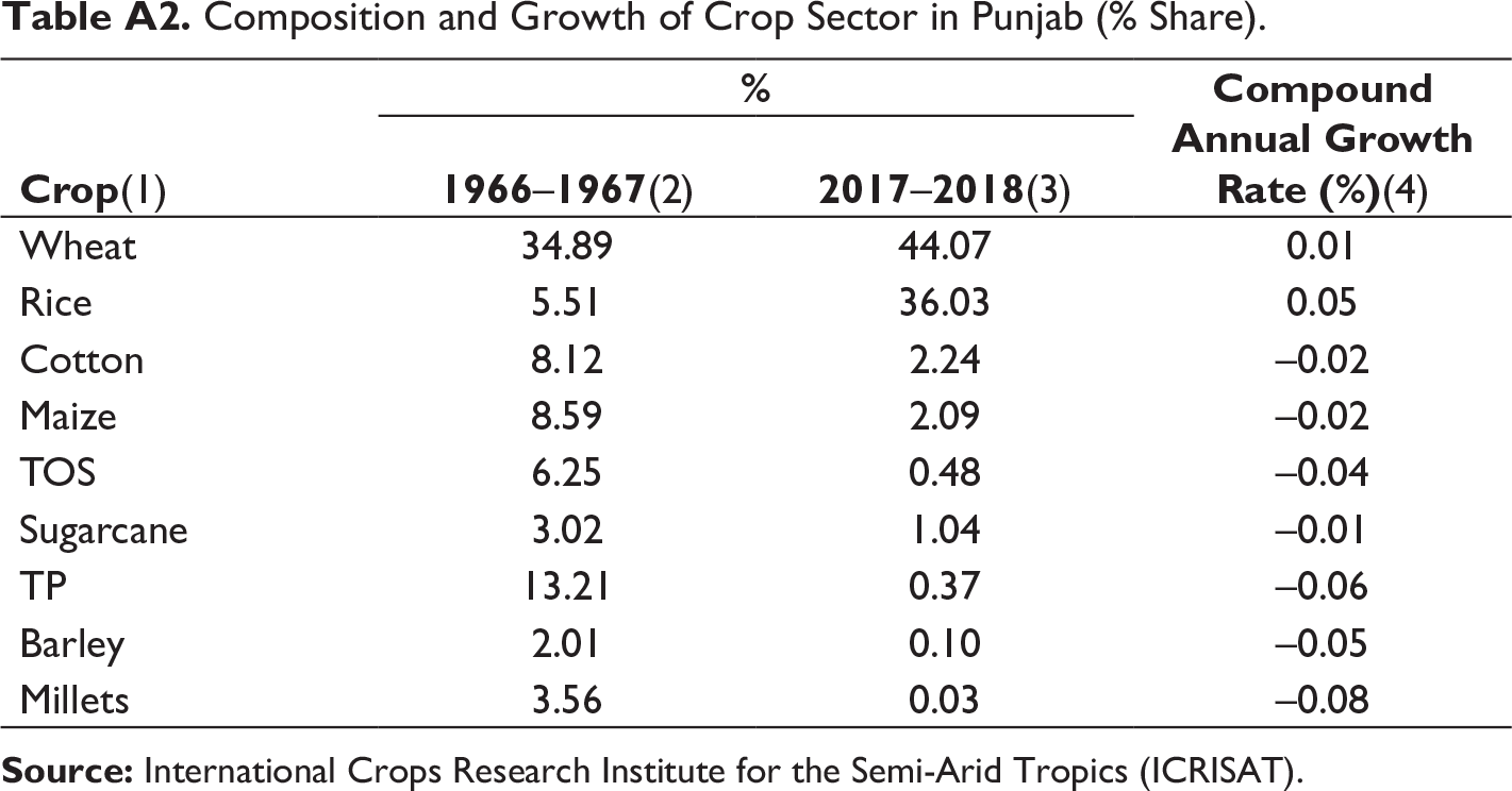
Among the Indian northern states, Punjab is an agriculturally rich state. Despite the state’s small geographical area (1.5% of the total area of the country), the GSDP of the agriculture sector increased by 5.7% per annum in 1971–1972 to 1985–1986, which is more than double of 2.31% of all-India growth in the same period (Gulati et al., 2017). The emergence of the green revolution has shown significant effect within the state, as a result the state attained self-sufficiency in food production. With the advent of the green revolution, wheat and rice have become major crops of the state and covered 44.07% and 36.03% of the cropped area in 2017–2018 against 30.26% and 4% in 1960–1961, respectively as shown in Appendix Table A2. It was the evolution of HYVs having better response to fertilisers, irrigation, pesticides and insecticides, and so on. The improved mechanisation such as plant protection, threshing, market, road, storage and processing further enhanced the production.

Nowadays, Punjab state faces declining trends in the share of agriculture sector to its economy. The state has lost its pre-eminent position of being the state with highest per capita income in the country. As shown in Table 1 contribution of agriculture and allied sectors to its state NSDP has declined continuously from 40.60% in 1970–1971 to 18.95% in 2018–2019. Conversely, contribution of industry and services sectors have increased from 17% and 42% in 1970–1971 to 25% and 46% in 2000–2001, and belonging to the same 26% and 55% in 2018–2019, respectively. Similarly, looking at the wheat and rice contribution to the central pool has also declined from 74% and 16% in 1970–1971 to 46.04% and 27.05% in 2016–2017 (GOI, 2018). Several studies observed that the low agricultural share in the state is mainly because farmers followed the same agriculture practices for last three-four decades, inadequate capital formation and low fertility rate of soil (Sidhu, 2002; Singh & Sidhu, 2004; Singh & Sidhu, 2006; Singh et al., 2008). So if current growth scenarios continue, it might be possible that the state slips further down among large Indian states in terms of its per capita income.

Table 1.

Sectoral Composition of NSDP in Punjab (in %).

Sr. N.	Sector	1970–1971	1980–1981	1990–1991	2000–2001	2010–2011	2018–2019
1	Agri. & allied	40.60	35.51	35.88	29.33	25.04	18.95
i	Agriculture	37.93	32.58	33.89	27.26	23.73	17.85
ii	Forestry and logging	2.64	2.90	1.91	1.81	1.09	0.91
iii	Fishing	0.03	0.03	0.08	0.26	0.22	0.19
iv	Mining & quarrying	0.03	0.01	0.01	0.00	0.02	0.09
2	Industry	17.32	16.76	20.51	24.83	29.77	26.02
3	Services	42.06	47.72	43.60	45.84	45.16	54.94
4	Per capita NSDP at 2004–2005 prices (₹)	11,993.2	16,087.9	21,028.3	27,241.4	44,769.3	61,600.5

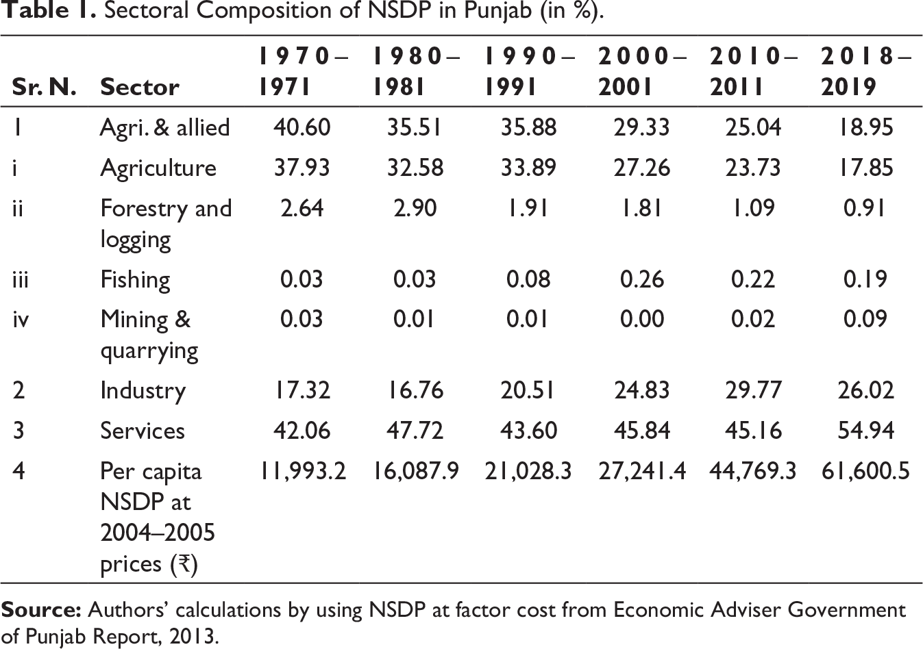
Source: Authors’ calculations by using NSDP at factor cost from Economic Adviser Government of Punjab Report, 2013.

Similarly, several other significant shifts have taken place over time, disparities in cropping pattern and inter-district variation in crop productivity also exist in the state. These differences can be attributed to the non-pro rata improvements in technologies of different crops and inter-regional variations in agro-infrastructure (Singh & Grover, 1991).

In particularly Punjab, several studies have investigated the pattern of agricultural productivity and diversification level within the state (Johl, 1996; Singh & Grover, 1991; Singh & Sidhu, 2004). However, only a few studies (Ray et al., 2005; Sajjad & Prasad, 2014) have addressed this issue at districts level of diversification and regional disparities, but no concrete attempts of addressing this matter of inter-regional disparities in crop diversification and agricultural productivity has been observed in the state. Being a small and one of the agriculturally rich states, it is important to see the disparities in cropping pattern and agricultural productivity at the regional level. This will lead to identify the micro-level problems of farm sector followed by appropriate policy formation. Against this background, the present article addresses the following issues: (a) What is the extent and nature of crop diversification and agricultural productivity in different regions within state? (b) What are the main drivers that spurred the process of crop diversification in different regions?

Our study contributes to the literature on crop diversification aspect; we find the performance of crop diversification and agricultural productivity in different regions, which may provide some ways to understand the causes of regional variation in crop pattern, and factors that affects the diversification and productivity level. This regional level measures provide valuable insights on the decision-making process faced by a farmer in adopting a cropping pattern. We extend the limited but growing literature on different types of crop diversification across regions within state.

The rest of the article is structured as follows: Section II presents a brief review of the literature. Section III presents the conceptual and theoretical framework. Section IV, results and discussion, and Section V present conclusions and policy implications.

Review of Literature

A detailed review of previous studies has been explained in this section to explore the historical trends and patterns of crop diversification in developing countries, including India. The review of relevant literature are given under two sections. The first section show reviews related to trend and pattern of crop diversification. The second section presents the literature on determinants of crop diversification and productivity.

Review Related to Trend and Pattern of Crop Diversification

Crop diversification is extensively used in current research works for agricultural development and rural development matters; however, its meaning can very often seem to be vague due to different definitions being encountered in various sources (Khatun & Thapa, 2015). Crop diversification refers to growing more than one or multiple crops in the same land in a particular season. It has discussed that different crops grow better in different agro-climatic conditions such as weather, soils texture. Joshi et al. (2004) made an attempt on pattern and determinants of agriculture diversification in South Asia and observed that the extent of diversification has been slow in most of the South Asian economies. It is because food security issues are still critical in the sub-continent; therefore, government policies are seemingly obsessed to encourage allocation of a large share of area to cereal crops for the purpose of self-sufficiency achieved in cereal. Moreover, Mahajan (2004) explained crop diversification in Kangra and found developed agriculture areas were comparatively more diversified as compared to less developed agriculture areas. The factors responsible for diversification in developed agriculture category include social factor (distance from education, age, education of head and family size), economic factor (income from farm, non-farm area, tenancy, tractor and farm size). In contrast, in underdeveloped agriculture category, the factors are tenancy, on farm and off farm income, and holding. Joshi et al. (2006) discussed the sources of agricultural growth in India and the role of diversification of high-value crops. They found that the growth of wheat and rice production have fallen, and more emphasis has been given to high-value crops. The study authorised grain-dominated northern and eastern region and found that price was the key source of growth. On the other side, in southern and western regions technology was main source of growth in crop income. However, diversification towards higher-value crops, that is, vegetables and fruit, accounted for about 27% of crop income growth in the 1980s and 31% in the 1990s. Further, as Birthal et al. (2007) explained, the measures of household participation in cultivation of fruits and vegetables are by farm size at the macro level. The study results showed that diversification of high-value crops increased the incomes of the farms, particularly in underdeveloped countries. The results described smallholders showed more involvement in high-value fruits and vegetable production compared to larger farms. Bhattacharyya (2008) has studied the pattern of crop diversification in South Asia and found that countries such as Bangladesh and Bhutan were moving toward specialisation in food grains. In contrast, countries like Nepal, Pakistan and India are slowly moving toward crop diversification. Among South Asian countries, the Maldives has attained a high level of diversification until the 1980s, but crop diversification has not been increased over time. The SID for West Bengal shows that the state is lagging behind the national average as the value of SID for India is 0.69, which is more than West Bengal, that is, 0.59 in 2004–2005. It does not mean that West Bengal is not diversifying in the crop because the SID has been increased from 0.52 in 1997–1998 to 0.59 in 2004–2005. Further, it was found that an increase in road length along with the adoption of technology in agriculture has been an important determinant of diversification. Dasgupta and Bhaumik (2014) explained the impact of crop diversification on the agriculture growth in West Bengal. The study has completely used secondary data and computed shares of the ‘expansion effect’ and ‘substitution effect’ in the total change of area under different crops from 1980–1981 to 2009–2010. The results revealed that given the study period, a major change in area under the crops like boro rice, oilseeds and potatoes occurred due to the substitution effect. Whereas, for aus, aman and pulses, the substitution effect has shown significantly negative and stronger than the expansion effect. However, fruits and vegetable have a strong and positive substitution effect as well as a positive expansion effect. Kumar and Gupta (2015) presents the trend and pattern of crop diversification in India during a period from 1990–1991 to 2011–2012. Simpson diversification index has shown the Indian agriculture is transforming from traditional survival agriculture to high-value agriculture, but it is not equally distributed across states as well as across different crop sub-sectors. The study also made efforts to know the determinants of crops diversification by using the fixed-effect model and found cropping intensity, average annual rainfall and gross irrigated area to be the major determinants of crop diversification. In particular, Punjab (Ray et al., 2005) has studied crop diversification based on soil and weather requirements of different crops in Punjab using GIS (Geographical information system). The analysis showed there is a need for diversifying wheat–rice cropping pattern, and need to increase the area under such crops that required fewer inputs and enrich soil health. Further, they analysed that south-western Punjab is suitable for low water requiring crops such as desi cotton, pearl millet, gram, and so on, whereas north-eastern Punjab with high rainfall and excess drainage should practice maize-based cropping system. Rice can be replaced by maize and other crops in central Punjab to control the exploitation of water.

Review Related to Determinants of Crop Diversification and Productivity

The extent of crop diversification is largely based on the geographic, climatic characteristics, socio-economic and technological accessibility of a region (Priyadarshini & Abhilash, 2019). A number of factors namely, resources related (that is, irrigation, climate change, soil health, etc.); technological factors (that is, seed quality, fertiliser, post-harvest processing, etc.); price factors (that is, inputs price, output price, profitability, procurement system, import and export, etc.); institutional factors (that is, size of land, government schemes, density of road, accessibility of market, irrigation, etc.); and household-specific factors (that is, knowledge, experience, capacity, resources base, food and feed requirement, etc.); are playing an important role to influence the area allocation pattern in a region (Alur & Maheswar, 2018). The major factors comprise need to augment income level among small holders (Birtha et al., 2013); price variations or crop failures (Alur & Maheswar, 2018); conservation of natural resources (Meynard et al., 2013); accessibility of production technologies (Vyas, 1996); higher profitability (Hazra, 2001); and, more important, mitigating the adverse impacts of climate change (McCord & Evans, 2015). The review of earlier studies identify the key factors namely, land size, family size, credit, access to extension services, type of tenancy, irrigation, education level of household that effects the nature and extent of crop diversification at the household level. Whereas, at aggregate level factors such as infrastructure development, profitability of crops, per capita income of consumers, input subsidy, and procurement system are impact the crop diversification (Anosike & Coughenour, 1990; Gupta & Tewari, 1985; Joshi et al., 2004; Pope & Presscott, 1980). However, Joshi et al. (2006) suggested that farm diversification is mainly directed by two forces, one is demand side factors, other is supply side factors. Therefore, specific factors observed are credit, irrigation, market infrastructure, road and transport facilities, procurement prices, and government policies on input subsidies. Ashfaq et al. (2008) examined the factors affecting farm diversification in Pakistan Punjab. The sample size for the study was 200 respondents from four villages, two of them close to the market and two of them away from the market. The main factors that are affecting diversification level are size of landholding, age, education, farming experience, off farm income, distance of farm from main road, market distance and farm machinery. A study has been conducted on determinants of crop diversification in Thailand by using primary as well as secondary sources. The study has taken 245 samples of both diversified farmers as well as non-diversified farmers and found that large farmers prefer mono-cropping pattern while small farmers tried to diversify cropping pattern. Labour shortage, market unavailability, soil suitability, lack of knowledge on growing other crop are some of the factors that restrict large farmers from diversifying (Kasem & Thapa, 2011). A study was forwarded by Rahman (2009) to elaborate the economic determinants of crop diversity in Bangladesh and identified that key drivers such as land size, owner operator, education of farmer, farmer’s membership in NGO’s, and developed infrastructure region positively affect the level of diversification, while it is negatively affected by less developed irrigation facility, fertiliser price and animal power service. Benin et al. (2003) analysed the determinants of cereal crop diversifying farms in the highlands of northern Ethiopia. Survey data are used to compare the determinants of inter and infra-specific diversity on household farms. Physical features of the farm and household characteristics such as livestock assets and the proportion of adults that are men have large and statistically significant effects on both the diversity of cereals. On the other side, demographic aspects such as age of household head and adult education levels affect only infra-specific diversity of cereals. Acharya et al. (2011) tried to identify the nature and extent of crop diversification in Karnataka for a period from 1982–1983 to 2007–2008. Composite entropy index (C.E.I.) has been used to know the extent of different crop groups. The results found that there is a rapid increase in diversification of commercial crops after WTO. Several infrastructural and technological factors negatively impact on crop diversification level. The adoption of basic infrastructural facilities like a sustained supply of irrigation water, fertiliser availability, markets, proper roads and transportation conditions are raising the process of agricultural development and crop diversification. The study also found that per capita income, the proportion of area under HYVs of cereals, proportion of urban population, proportion of gross irrigated area to gross cropped area, rainfall, average size of holding, market density and fertiliser consumption are the major factors accountable for the changes in crop diversification. Kumar et al. (2012) explained the determinants of crop diversification in four eastern states (Bihar, Jharkhand, Odisha and West Bengal) of India. Tobit regression model outcomes show that education, modern implements and road connectivity are major factors of crop diversification. Similarly, Basavaraj et al. (2016) explained nature and factors that influenced crop diversification at the micro-level under two distinct agro-climatic conditions in Gadag district. The primary data were collected from 30 samples in 1997, and the secondary data pertaining to the area under important crop groups were obtained for the period from 1998–1999 to 2011–2012. The results shows the growth rate is higher for area under horticultural crops and pulses as compared to area under cereals, oilseeds, fibre and other crop groups. The estimation has shown that share of cereal crop groups has decreased significantly from 32.53% to 28.81% and that of fruits and vegetables has increased considerably from 0.10% to 0.25% for fruits and from 4.66% to 7.80% for vegetables. Further, size of landholding, gross irrigated area and net return realised per farm are the major factors that influenced crop diversification. In context of Odisha as Nayak and Kumar (2019) assessed the structure and nature of cropping pattern, crop diversification, productivity level and inter-district disparity by using the Herfindahl index, location quotient and Gini coefficient study and found that majority of the districts in state are experiencing a lateral movement towards crop specialisation.

In brief, it was observed that the cropping pattern has been changed over time due to changing demand for different food items. Overall depiction at international level, national and state-specific, based on the review of available literature shows that till the 1980s, the trends moved towards cereals, particularly to wheat and rice. It was mainly because of the advent of green revolution technologies and to meet the domestic demand for staple foods. However, from 1990s onwards, relative share in acreage under coarse cereals and pulses have declined and that of fruits and vegetables have increased substantially as a response to integrating the local markets with global markets during post WTO era. It is noticed that the cropping pattern change has not occurred simultaneously in all regions within state or country. In particular, variations in change patterns have been observed in specific region, some of the regions have experienced lateral movements towards cropping pattern. It is governed mainly by the agro-ecological and technological factors in a particular area. Therefore, crop diversification depends on various factors such as natural, man-made and socio-economic environments. Understanding the behaviour of farmers towards cropping pattern and how they influence their crop diversification decisions would help policymakers in making precise measures for promoting crop diversification.

Data and Methodology

Data

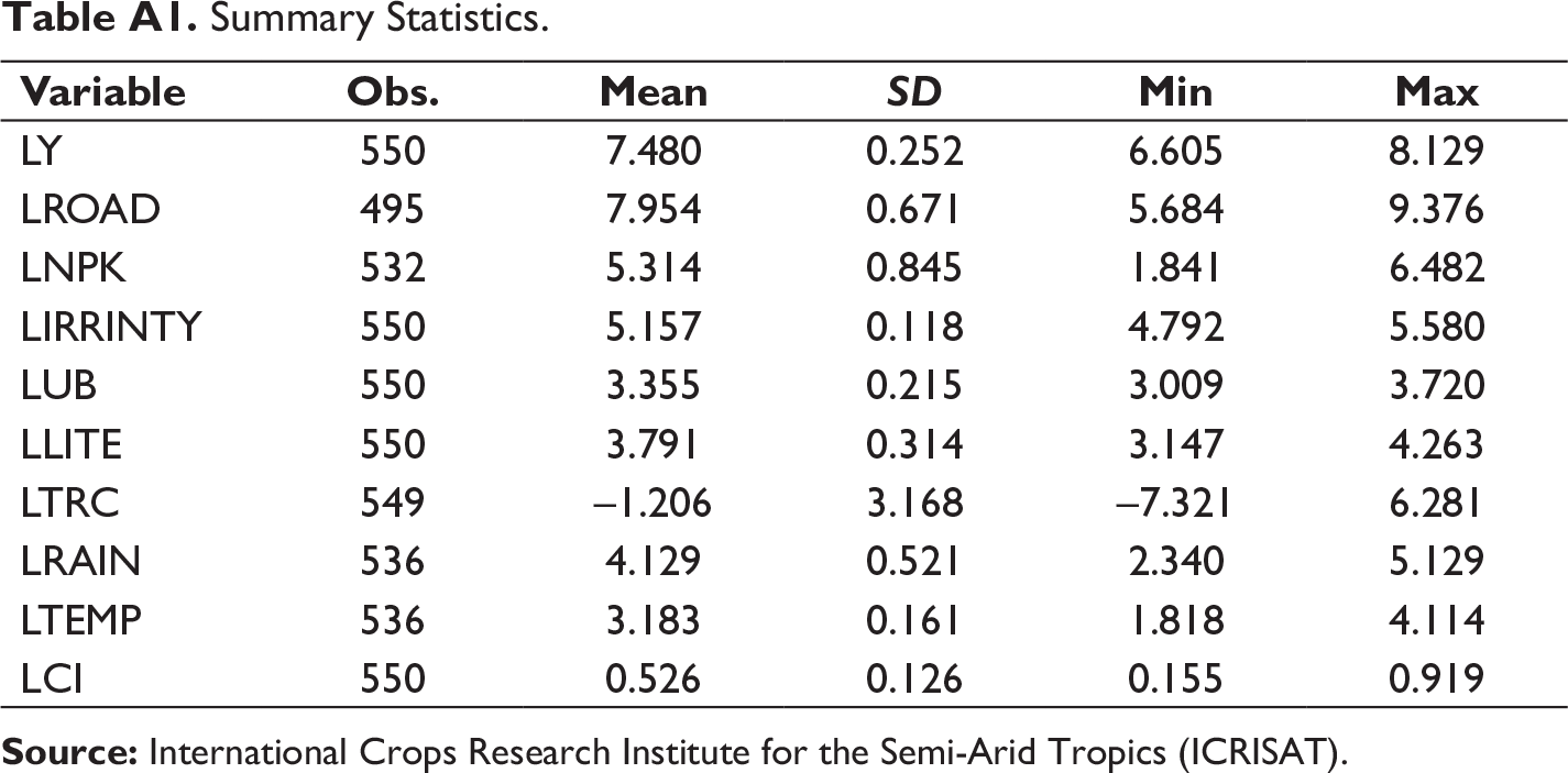
The present study is primarily based on secondary data collected from VDSA (Village dynamics in south Asia) dataset generated by International Crops Research Institute for the Semi-Arid Tropics (ICRISAT). Data for the major nine crops, namely wheat, maize, cotton, paddy, total oilseeds, sugarcane, total pulses, barley and millets (Bajra) were collected separately for various districts covering the period 1966–1967 to 2017–2018, which together accounted for 80% of gross cropped area. The summary statistics of the variables were presented in Table A1. Recently, Punjab state was divided into 22 districts as 11 new districts were merged with the parent districts. The districts in this database relate to the 1966 base, that is, data of districts formed after 1966 are given back to their parent districts. Based on agro-climatic conditions, infrastructure and technology development in the farm sector, the districts were divided into four zones, namely, Zone-I traditional rice belt, Zone-II cotton belt, Zone-III central districts and Zone-IV semi hilly area.

Methodology

To accomplish the compound growth rate of area under each crop over time we fit the semi-log function: In the semi-log function the slope coefficient measures the constant proportional or relative change in dependent variable (Y) for a given absolute change in the value of the explanatory variable (t).

\ln Y = a + b t

lnY = dependent variable (area under different crops), a = intercept, b = coefficient of time

Measures of Crop Diversification

Crop diversification can be measured by various statistical indices, namely index of maximum proportions, Gibbs and martin index, Herfindahl index, Ogive index, Simpson index, entropy index, Shannon diversity index many more, few of the methods explain either concentration or diversification of crops over time and space. Each method has some limitation or superiority over the other (Shiyani & Pandya, 1998). For assessing the extent of crop diversification, composite entropy index (C.E.I) was used in the present analysis, formerly used by (Acharya et al., 2011; Shiyani & Pandya, 1998). C.E.I. was preferred over other competing indices, because it processes all desirable properties of modified entropy index and it is used to compare diversification across situation having different and large number of activities since it gives due importance to the number of activities. Since index uses –log_NP as weights, it assigns more to lower quantity and less weight to higher quantity. The formula of calculating C.E.I. is given by:

C .E .I = - (\sum_{i = 1}^{N} P * \log_{N} P_{i}) * \{1 - (1 / N)\}

(1)

The C.E.I. has two components, namely, distribution and number of crops, or diversity. The value of C.E.I. increases with the decrease in concentration and rises with the number of crops. Both the components of the index are bounded by zero and one, and thus the value of C.E.I. range between 0 and 1.

Agricultural Productivity

To compute agricultural productivity, we used a methodology that is earlier applied by Nayak and Kumar (2019) and Sapre and Deshpande (1964). This method is generally used because, along with crop yield level’s rank, that includes the proportion of area under crop, the weighted average of ranks is used instead of simple average ranks. The lower value of the index implies a higher level of productivity. It means that if a district’s yield level of rice is highest in the state, it will get weightage 1 whereas if a district’s yield level of rice is ranked 10^th in the state, it will get weightage 10. The formula for calculating this index can be expressed as:

Spare and Deshpande index = \frac{r_{1 i} p_{1 i} + r_{2 i} p_{2 i} ................... + r_{n i} p_{n i}}{p_{1 i} + p_{2 i} ............. + p_{n i}}

(2)

where, r₁… … . . + r _n represent the rank of crops as per their yield level in the district ‘i’ in comparison to other district and p₁ ... … . + p_n represent the proportion of area devoted to these crops in the district ‘i’.

Empirical Specification

To estimates the factors that affect the level of productivity as the following specification:

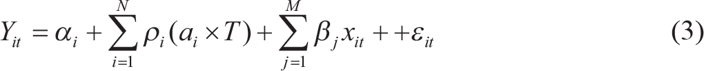
Y_{i t} = α_{i} + \sum_{i = 1}^{N} ρ_{i} (a_{i} \times T) + \sum_{j = 1}^{M} β_{j} x_{i t} + + ε_{i t}

(3)

where, Y_it is dependent variables (log of productivity for different crops & diversification index) in district i in year t. α_i represents the district fixed effect. Further, (a_i × T) is a district-specific exponential time trend to switch for the district-specific heterogeneity in productivity growth due to others technological change. ρ_i is coefficient of time trend across districts. The β’s are coefficients of different x_it explanatory variables in districts i in year t.

Result and Discussion

Growth and Extent of Cropping Pattern in Different Agro-climatic Zones

The growth rate of area under crops produces in different zone is presented in Table 2. Almost in all zone only two crops such as rice and wheat have shown positive and statistically significant growth throughout the study period. However, the other selected crops namely, maize, millets, barley, pulses, oilseed, sugarcane and cotton have shown significant but negative growth during same period. The highest growth rate under an area is achieved by rice crop in Zone-II around 6%, followed by Zone-III 4.44%, Zone-IV 3.09% and Zone-I 2.71% during whole period. Similarly, in case of area under wheat the highest growth rate attainted by Zone-II about 1.36% followed by Zone-I (1.07%), Zone-IV (0.73%) and Zone-III (0.47%), respectively. The findings implying that these two crops have been sown on maximum areas in the state, it might be the policy of assured prices, market support price and free electricity in case of these crops.

Table 2.

Zone-wise Growth Rates of Area Under Different Crops.

Crops	TRB Zone-I	CB Zone-II	CD Zone-III	SHA Zone-IV	Overall Punjab
LRice	2.71*** (0.0018)	6.01*** (0.0037)	4.44*** (0.0039)	3.09*** (0.0012)	4.26*** (0.0027)
LWheat	1.07*** (0.0009)	1.36*** (0.0009)	0.47*** (0.0009)	0.73*** (0.0007)	1.02*** (0.0008)
LMaize	–4.17*** (0.0012)	–12.34*** (0.0096)	–5.51*** (0.0023)	–0.57*** (0.0009)	–3.41*** (0.0014)
LMillets	–9.11*** (0.0118)	–11.36*** (0.0043)	–2.83*** (0.0097)	–3.2*** (0.0092)	–9.13*** (0.0047)
LBarley	–11.12*** (0.0118)	–4.37*** (0.0031)	–3.99*** (0.0031)	–4.92*** (0.0068)	–4.65*** (0.0027)
LPulses	–5.26*** (0.0038)	–8.94*** (0.0032)	–6.15*** (0.0025)	–9.92*** (0.0064)	–9.14*** (0.0038)
LOilseed	–3.35*** (0.0038)	–4.87*** (0.0037)	–8.42*** (0.0049)	–1.3*** (0.0044)	–5.65*** (0.0035)
LSugarcane	–0.02*** (0.0019)	–3.32*** (0.0042)	–1.31*** (0.0023)	0.88*** (0.0018)	–0.61*** (0.0019)
LCotton	–8.68*** (0.0062)	–0.02 (0.0025)	–9.17*** (0.0056)	–12.05*** (0.0104)	–0.49*** (0.0022)

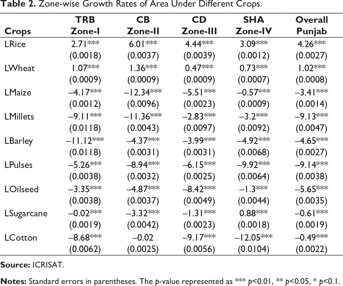
Source: ICRISAT.

Notes: Standard errors in parentheses. The p-value represented as *** p<0.01, ** p<0.05, * p<0.1.

Table 3 presents the temporal structure of cropping pattern in the different agro-climatic zone. It shows that even though all four zones are specialised in a few crop produce but some of them are less or some are more specialised according to their degree of diversification score. In the Zone II cotton belt, the districts covered Bathinda, Sangrur and Jalandhar were revealed as more specialised as compared to other three zones. Zone I includes the districts Gurdaspur, Amritsar and Kapurthala, are specialised in few crops but less than the cotton belt. Similarly, Zone IV also moved towards specialisation but still a less specialised zone compared to the other three zones. The higher value of the index relatively indicates that there exists diversification in the initial years of study in every zone. In recent years less diversification was seen in almost all zones, which is attributed mainly to the only wheat–rice cropping pattern dominating in each zone. Hence, it indicates most of the areas in the state are experiencing a lateral movement toward crop specialisation and crop diversification is not happening. The shift of crops has mostly taken place towards paddy in most districts of the state.

Table 3.

Diversification Level in Different Zone.

Year	1966	1970	1980	1990	2000	2010	2018	% Change
Zone I (traditional rice belt)	0.58	0.54	0.45	0.38	0.37	0.32	0.34	–42.44
Gurdaspur	0.62	0.58	0.48	0.42	0.40	0.36	0.38	–37.05
Amritsar	0.60	0.51	0.45	0.37	0.36	0.29	0.31	–49.54
Kapurthala	0.53	0.54	0.42	0.35	0.35	0.31	0.32	–40.59
Zone II (cotton belt)	0.62	0.58	0.56	0.46	0.42	0.37	0.29	–53.38
Ferozepur	0.62	0.59	0.53	0.47	0.43	0.38	0.29	–53.59
Bathinda	0.60	0.56	0.58	0.48	0.46	0.41	0.28	–52.17
Sangrur	0.64	0.59	0.58	0.42	0.37	0.33	0.29	–54.29
Zone III (central districts)	0.59	0.51	0.50	0.39	0.37	0.32	0.32	–46.06
Jalandhar	0.54	0.48	0.46	0.41	0.40	0.36	0.35	–34.79
Ludhiana	0.58	0.49	0.54	0.39	0.36	0.30	0.31	–46.97
Patiala	0.65	0.56	0.50	0.36	0.34	0.31	0.29	–54.66
Zone IV (semi hilly areas)	0.58	0.56	0.53	0.49	0.48	0.41	0.43	–26.10
Hoshiarpur	0.56	0.53	0.48	0.48	0.48	0.43	0.45	–18.16
Rupnagar	0.60	0.60	0.58	0.51	0.47	0.39	0.40	–33.41

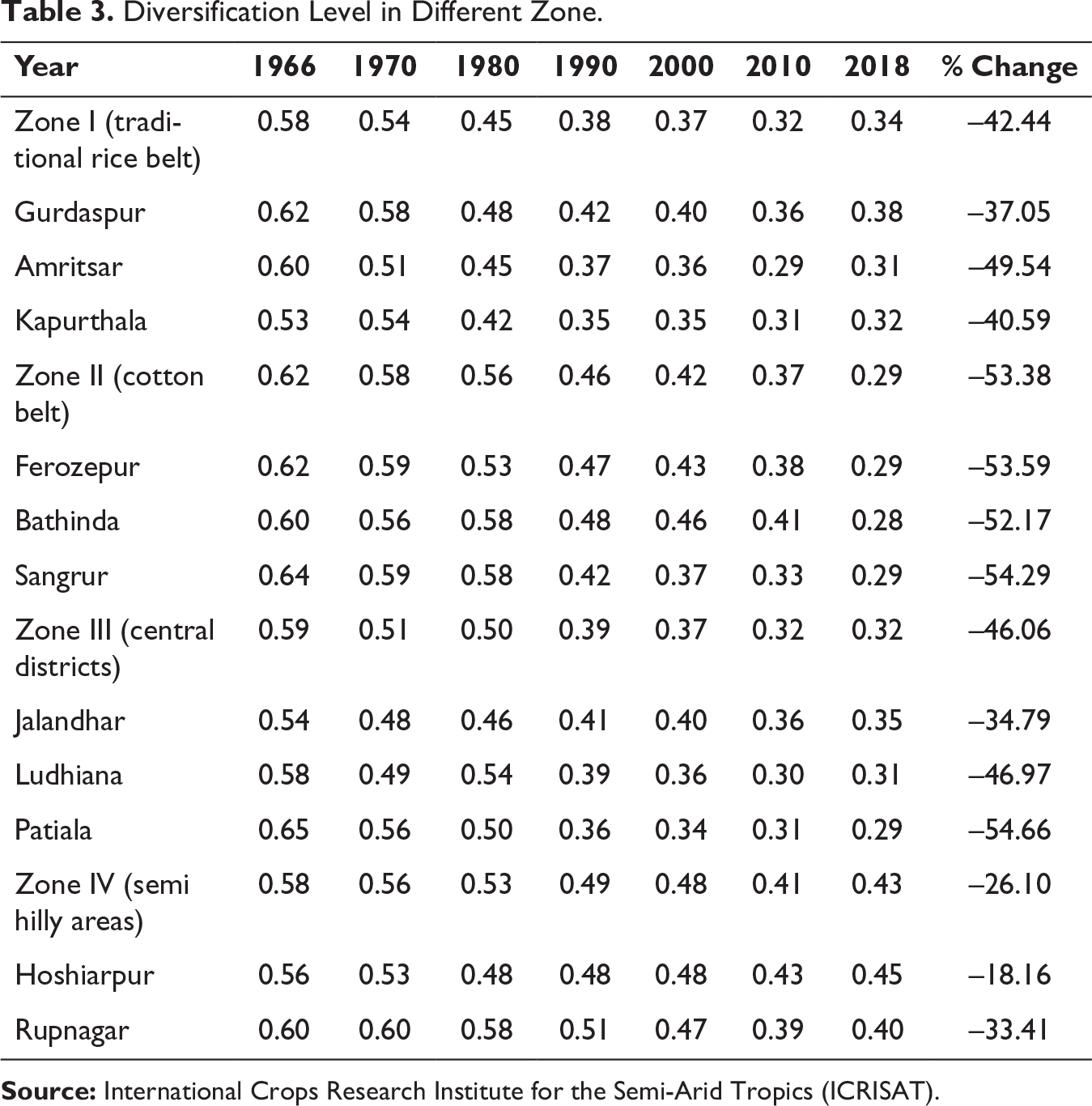
Source: International Crops Research Institute for the Semi-Arid Tropics (ICRISAT).

Productivity Level and Inter-district Disparities

Table 4 depicts the ranking of the districts in productivity from 1966–2018 in Punjab. The value of different districts captures important characteristics of inter-district variations in Punjab’s agricultural productivity. It is indicated that the districts, Jalandhar, Kapurthala and Amritsar, which had higher agricultural productivity in 1966–1970, obtained lower SDI value in 2011–2018. Conversely, the districts namely, Sangrur, Ferozepur who ranked moderate in 1966–1970, turn out to be higher agricultural productivity districts in 2011–2018. The district Hoshiarpur with lower rank in 1966–1970 had achieved moderate position in 2011–2018. The case of Ludhiana is, however unique. It can be seen that with respect to SDI value the district rank almost first throughout the study period in the whole state. The districts Gurdaspur and Rupnagar have less agricultural productivity throughout the study period. Further clarifications can be made on the graph over the temporal behaviour of Punjab by districts. The difference in productivity is clearly noticeable by the radar diagram (Figure 1). The points closer to the centre in Figure 1 are more productive. The points far away from the centre in the diagram are less productive. In the diagram, the distance from the centre to the radius is 12 unit.

Table 4.

Rank of Districts as per Productivity Index, 1966–2018.

Ranking	1966–1970		1971–1980		1981–1990		1991–2000		2001–2010		2011–2018
Ranking	Districts	SDI	Districts	SDI	Districts	SDI	Districts	SDI	Districts	SDI	Districts	SDI
1	Ludhiana	1.39	Ludhiana	1.75	Ludhiana	1.55	Ludhiana	1.56	Ludhiana	1.55	Sangrur	2.55
2	Jalandhar	3.51	Sangrur	2.70	Sangrur	2.30	Sangrur	1.73	Sangrur	1.61	Ludhiana	3.53
3	Kapurthala	3.71	Jalandhar	3.75	Patiala	3.62	Patiala	4.46	Patiala	3.49	Ferozepur	3.67
4	Amritsar	3.76	Ferozepur	4.37	Jalandhar	4.01	Ferozepur	4.59	Ferozepur	4.54	Hoshiarpur	4.12
5	Bathinda	4.45	Bathinda	4.84	Ferozepur	4.55	Jalandhar	5.03	Bathinda	5.05	Jalandhar	4.61
6	Sangrur	5.18	Amritsar	4.82	Bathinda	5.27	Bathinda	5.61	Jalandhar	5.33	Bathinda	4.68
7	Patiala	5.36	Kapurthala	6.08	Kapurthala	7.24	Kapurthala	7.32	Kapurthala	6.38	Patiala	4.98
8	Ferozepur	5.84	Patiala	6.17	Amritsar	7.60	Amritsar	6.76	Amritsar	8.34	Kapurthala	7.36
9	Gurdaspur	8.89	Rupnagar	8.10	Rupnagar	8.97	Hoshiarpur	8.81	Rupnagar	8.91	Rupnagar	7.97
10	Hoshiarpur	9.15	Hoshiarpur	8.89	Hoshiarpur	9.35	Rupnagar	8.85	Gurdaspur	9.10	Amritsar	8.91
11	Rupnagar	9.88	Gurdaspur	9.83	Gurdaspur	9.36	Gurdaspur	9.71	Hoshiarpur	9.10	Gurdaspur	10.48

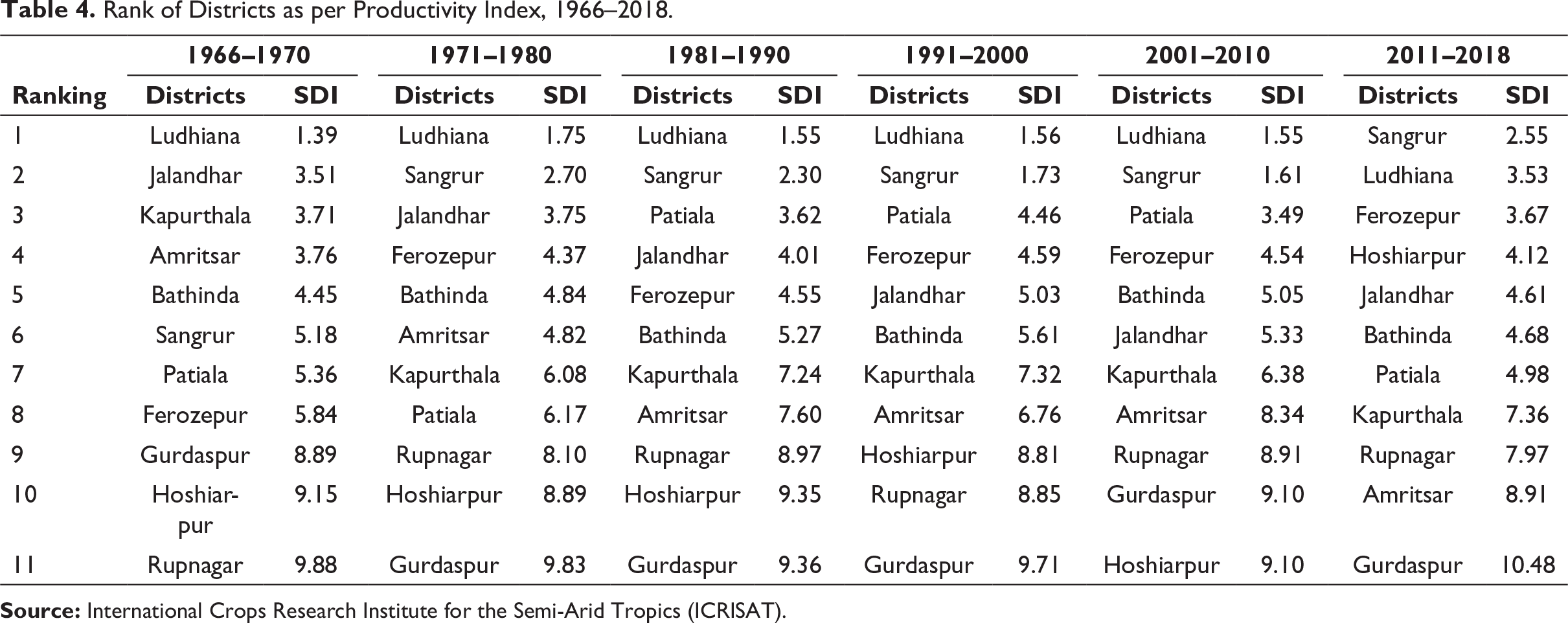
Source: International Crops Research Institute for the Semi-Arid Tropics (ICRISAT).

Figure 1.

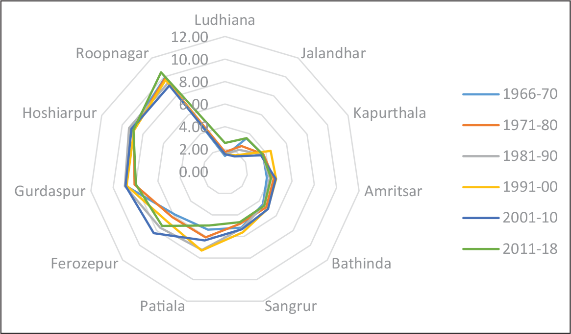
Source: Based on Table 4.

Model Specification Tests

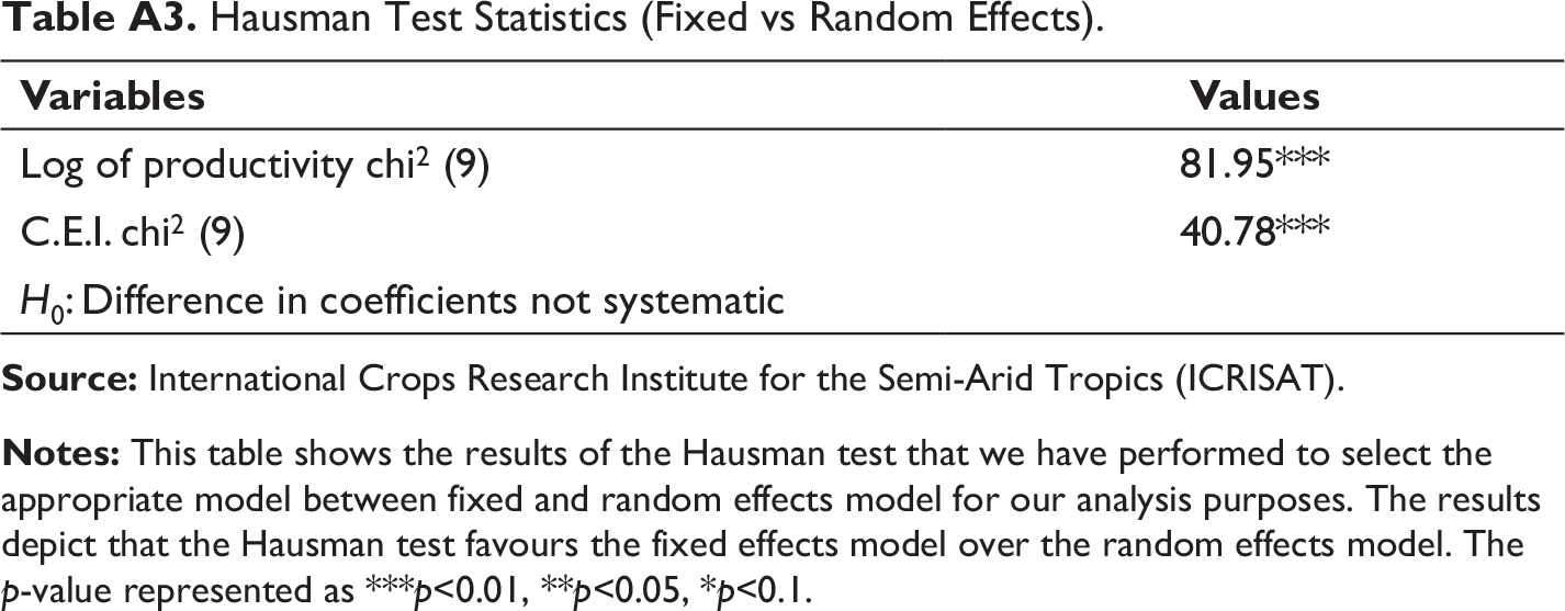
To identify the suitable model on panel data analysis for estimating the impact of different explanatory variables on productivity as well as on diversification level, we pursue the Hausman test that favour the fixed effects model as specification shown in ****Table A3. The test rejected the null hypothesis that contains random effect model as appropriate, therefore our results favour the fixed effect regression model with district-specific trend.

Robustness Check

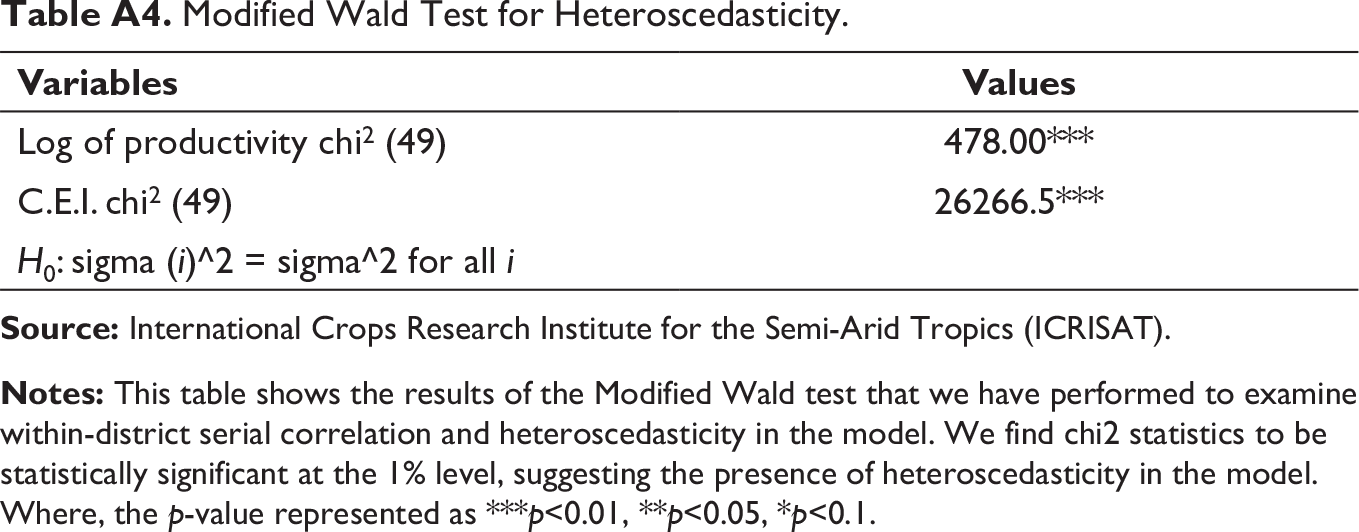
Further, we used Modified Wald test for heteroscedasticity as shown in ****Table A4. In estimation, we found that the chi2 statistics is significant at 1% level, postulating the presence of heteroscedasticity. Therefore, to detect within-district heteroscedasticity and serial correlation, the standard errors have been clustered at the district level.

Determinants of Productivity

Table 5 presents the estimations of both pooled OLS and fixed effects model to identify the relationship between productivity and explanatory variables such as log of road, fertiliser, irrigation intensity, literacy, tractor, rainfall, temperature and cropping intensity. To avoid the problem of multicollinearity, mean value of variance inflationary factor (VIF) has been estimated as 2.22 showing no multicollinearity. The overall significance of the F value is quite satisfactory. All explanatory variables are showing positive and statistically significant relation with productivity except irrigation intensity. Irrigation intensity shows a significant but negative relationship with productivity.

Table 5.

Estimated Regression Coefficients of Equation (3).

Variables	(1)	(2)
	Productivity
	Pooled OLS	Fixed Effects
LROAD	0.0628***	0.1109***
	(0.0124)	(0.0169)
LNPK	0.0763***	0.1412***
	(0.0170)	(0.0258)
LIRRINTY	–0.2583**	–0.1908**
	(0.1035)	(0.0853)
LUB	0.2253***	0.6263***
	(0.0405)	(0.0499)
LLITE	0.1707***	1.1607***
	(0.0398)	(0.1237)
LTRC	0.0011	0.0013
	(0.0019)	(0.0012)
LRAIN	0.0142	0.0264**
	(0.0128)	(0.0127)
LTEMP	0.0452	0.0460
	(0.0290)	(0.0275)
LCI	0.5720***	0.3616**
	(0.1615)	(0.1519)
Constant	6.0024***	–0.0614
	(0.5698)	(0.8001)
Observations	474	474
Number of year		49
R-squared	0.6904	0.4507
Adjusted R-squared	0.684	0.440
F-stat	100.4	50.48

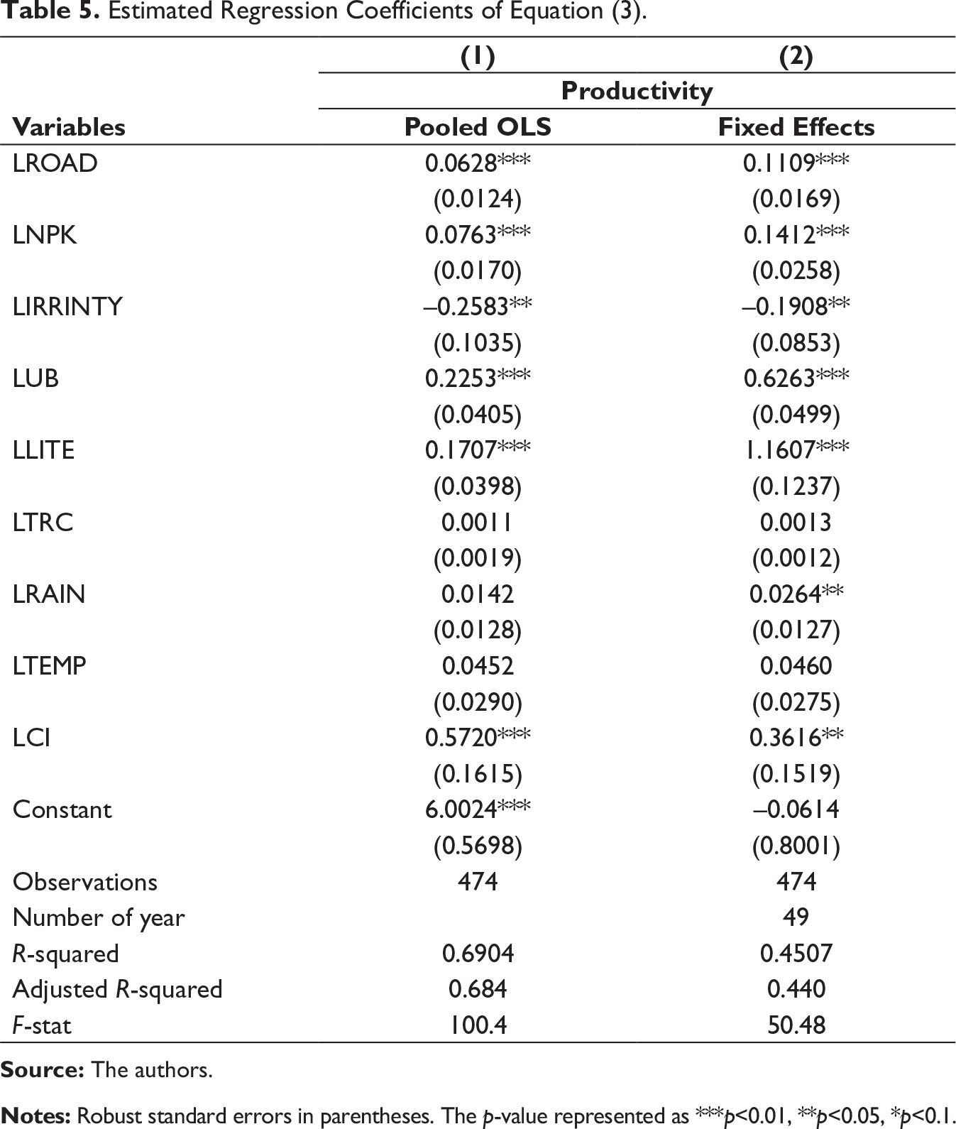
Source: The authors.

Notes: Robust standard errors in parentheses. The p-value represented as ***p<0.01, **p<0.05, *p<0.1.

Determinants of Crop Diversification

Table 6 presents the factors that affect the level of diversification. The results found that the variables market, road, urbanisation, tractor and rain have a statistically significant and positive impact on diversification as expected. Whereas the fertiliser (NPK), intensity of irrigation and cropping intensity have a negative impact on crop diversification in the state.

Table 6.

Estimated Regression Coefficients of Equation (3).

Variables	(1)	(2)
	Composite Entropy Index
	Pooled OLS	Fixed Effects
LMARKT	0.0199***	0.0471***
	(0.0072)	(0.0105)
LROAD	0.0237***	0.0228***
	(0.0039)	(0.0033)
LNPK	–0.0690***	–0.0622***
	(0.0063)	(0.0088)
LIRRINTY	–0.0947***	–0.0623**
	(0.0248)	(0.0259)
LUB	0.0337**	0.0341***
	(0.0139)	(0.0090)
LTRC	0.0020***	0.0024***
	(0.0007)	(0.0004)
LRAIN	0.0197***	–0.0749
	(0.0044)	(0.0456)
LCI	–0.0912**	1.1866***
	(0.0451)	(0.1738)
Constant	1.1179***
	(0.1544)	438
		49
Observations	435	0.3902
Number of year	0.7118	0.380
R-squared	0.706	0.4398
Adjusted R-squared	117.6	0.428
F-stat	–0.0199***	64.46

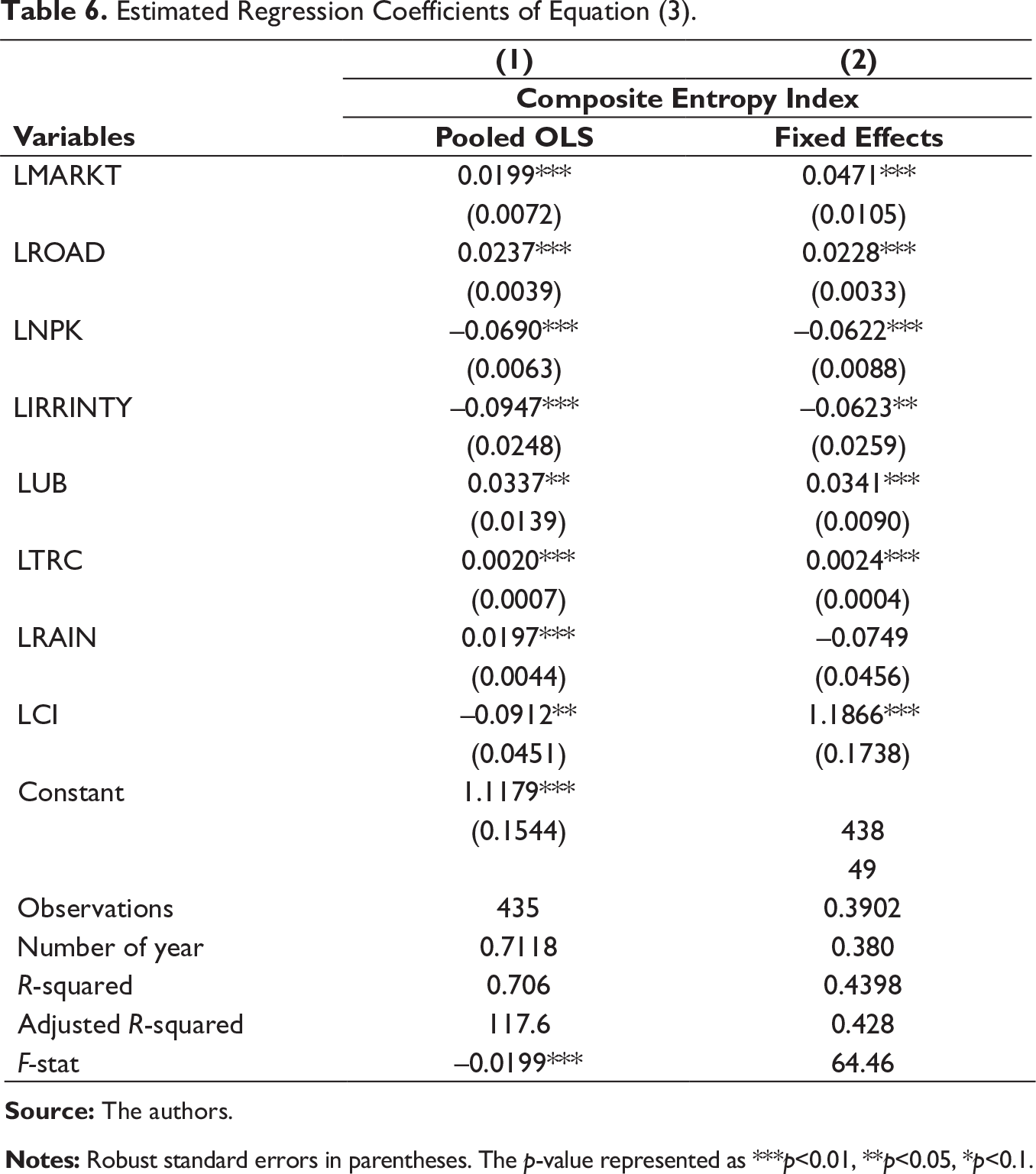
Source: The authors.

Notes: Robust standard errors in parentheses. The p-value represented as ***p<0.01, **p<0.05, *p<0.1.

Conclusion

In Punjab, the process has been changed in agriculture, and it moves towards few (wheat and rice) crops only in all zones. It showed that almost in all zones only two crops, such as rice and wheat, have shown positive and statistically significant growth throughout the study period. The findings imply that these two crops have been sown on maximum areas in the state. It was a substitution shift from other crops, that is, pulses, barley and oilseed. From the estimation, it was found that the four zones are specialised in few crops, but some of them are relatively less or some are more. Hence, we found that some of them had experienced a lateral movement toward crop specialisation and crop diversification is not happening. Further, it was found that the districts Jalandhar, Kapurthala and Amritsar who have higher rank in agricultural productivity in 1966–1970 had reduced to a lower rank value in 2011–2018. Conversely, the districts namely Sangrur and Ferozepur which have ranked moderate in 1966–1970, turn out to be higher agricultural productivity districts in 2011–2018. The district Hoshiarpur with lower rank in 1966–1970 had achieved moderate position in 2011–2018. In case of Ludhiana is, however, unique. It can be seen that in respect to SDI value, the district rank almost first throughout the study period in the whole state. The districts Gurdaspur and Rupnagar have less agricultural productivity throughout the study period. Further, regression results had identified the main drivers that enhance the level of productivity are better infrastructure such as road, fertiliser, urbanisation, literacy and cropping intensity. Similarly, the study also investigate the factors that influenced crop diversification level. The key factors such as accessibility of market and roads have a positive influence on crop diversification. Whereas, more use of fertiliser, intensity of irrigation, and rainfall have led to concentration rather than crop diversification. As the analysis indicates that there is need to emphasise on agro-climatic regional preparation by clearly identifying the existing resource endowments and constraints of the agro-climatically homogeneous regions. The farmers will switch over to alternative crops only when they will be sure of getting higher profit from the new crops.

Footnotes

Appendix

Table A1. Summary Statistics.

Variable	Obs.	Mean	SD	Min	Max
LY	550	7.480	0.252	6.605	8.129
LROAD	495	7.954	0.671	5.684	9.376
LNPK	532	5.314	0.845	1.841	6.482
LIRRINTY	550	5.157	0.118	4.792	5.580
LUB	550	3.355	0.215	3.009	3.720
LLITE	550	3.791	0.314	3.147	4.263
LTRC	549	–1.206	3.168	–7.321	6.281
LRAIN	536	4.129	0.521	2.340	5.129
LTEMP	536	3.183	0.161	1.818	4.114
LCI	550	0.526	0.126	0.155	0.919

Source: International Crops Research Institute for the Semi-Arid Tropics (ICRISAT).

Table A2. Composition and Growth of Crop Sector in Punjab (% Share).

Crop(1)	%		Compound Annual Growth Rate (%)(4)
Crop(1)	1966–1967(2)	2017–2018(3)	Compound Annual Growth Rate (%)(4)
Wheat	34.89	44.07	0.01
Rice	5.51	36.03	0.05
Cotton	8.12	2.24	–0.02
Maize	8.59	2.09	–0.02
TOS	6.25	0.48	–0.04
Sugarcane	3.02	1.04	–0.01
TP	13.21	0.37	–0.06
Barley	2.01	0.10	–0.05
Millets	3.56	0.03	–0.08

Source: International Crops Research Institute for the Semi-Arid Tropics (ICRISAT).

Table A3. Hausman Test Statistics (Fixed vs Random Effects).

Variables	Values
Log of productivity chi² (9)	81.95***
C.E.I. chi² (9)	40.78***
H₀: Difference in coefficients not systematic

Source: International Crops Research Institute for the Semi-Arid Tropics (ICRISAT).

Notes: This table shows the results of the Hausman test that we have performed to select the appropriate model between fixed and random effects model for our analysis purposes. The results depict that the Hausman test favours the fixed effects model over the random effects model. The p-value represented as ***p<0.01, **p<0.05, *p<0.1.

Table A4. Modified Wald Test for Heteroscedasticity.

Variables	Values
Log of productivity chi² (49)	478.00***
C.E.I. chi² (49)	26266.5***
H₀: sigma (i)^2 = sigma^2 for all i

Source: International Crops Research Institute for the Semi-Arid Tropics (ICRISAT).

Notes: This table shows the results of the Modified Wald test that we have performed to examine within-district serial correlation and heteroscedasticity in the model. We find chi2 statistics to be statistically significant at the 1% level, suggesting the presence of heteroscedasticity in the model. Where, the p-value represented as ***p<0.01, **p<0.05, *p<0.1.

Acknowledgement

The authors are thankful to the anonymous referee for his comments on the earlier version of this article.

Declaration of Conflicting Interests

Funding

The authors received no financial support for the research, authorship and/or publication of this article.

ORCID iD

Poonam Rani

References

Acharya

S. P.

Basavaraja

Kunnal

L. B.

Mahajanashetti

S. B.

Bhat

A. R.

(2011). Crop diversification in Karnataka: An economic analysis. Agricultural Economics Research Review , 24, 351–358.

Alur

A. S.

Maheswar

D. L.

(2018). Crop diversification-a strategy to improve agricultural production. PNASF News , 8, 1–14.

Anosike

Coughenour

C. M.

(1990). The socioeconomic basis of farm enterprise diversification decisions 1. Rural Sociology , 55(1), 1–24.

Ashfaq

Hassan

Naseer

M. Z.

Baig

I. A.

Asma

(2008). Factors affecting farm diversification in rice-wheat. Pakistan Journal of Agricultural Sciences , 45(3), 91–94.

Basavaraj

N. D.

Gajanana

T. M.

Satishkumar

(2016). Crop diversification in Gadag district of Karnataka. Agricultural Economics Research Review , 29(1), 151.

Benin

Smale

Gebremedhin

Pender

Ehui

S. K.

(2003 August 16–22). The determinants of cereal crop diversity on farms in the Ethiopian highlands [Paper Presentation]. 25th International Conference of Agricultural Economists.

Bhattacharyya

(2008, May). Crop diversification: A search for an alternative income of the farmers in the state of West Bengal in India. In International Conference on Applied Economics–ICOAE (pp. 83–94).

Birthal

P. S.

Joshi

P. K.

Roy

Thorat

(2007). Diversification in Indian agriculture towards high value crops: The role of small holders. Washington DC: The international food policy research institute.

Birthal

P. S.

Joshi

P. K.

Roy

Thorat

(2013). Diversification in Indian agriculture toward high-value crops: The role of small farmers. Canadian Journal of Agricultural Economics/Revue Canadienne d’agroeconomie, 61(1), 61–91.

10.

Dasgupta

Bhaumik

S. K.

(2014). Crop diversification and agricultural growth in West Bengal. Indian Journal of Agricultural Economics , 69(1), 107–124.

11.

Economic Survey. (2017–18). Economic and Statistical Organization, Government of Punjab.

12.

Gulati

Roy

Hussain

(2017). Getting Punjab agriculture back on high growth path: Sources, drivers and policy lessons. Indian Council for Research on International Economic Relations (ICRIER), New Delhi, India.

13.

Gupta

R. P.

Tewari

S. K.

(1985). Factors effecting crop diversification: An empirical analysis. Indian Journal of Agricultural Economics, 40(902–2018–2395), 304–309.

14.

Hazra

C. R.

(2001). Crop diversification in India. Crop diversification in the Asia-Pacific Region. Papademetriou

Minas K.

, & Dent

Frank J.

(Eds.). Food and Agriculture Organization of the United Nations. Regional Office for Asia and the Pacific (pp.32–50). Bangkok, Thailand.

15.

Johl

S. S.

(1996). Future of agriculture in Punjab: Some policy issues. Journal of Agricultural Development and Policy , 7(1), 1–21.

16.

Joshi

A. K.

Mishra

Chatrath

Ferrara

G. O.

Singh

R. P.

(2007). Wheat improvement in India: Present status, emerging challenges and future prospects. Euphytica, 157(3), 431–446.

17.

Joshi

P. K.

Gulati

Birthal

P. S.

Tewari

(2004). Agriculture diversification in South Asia: Patterns, determinants and policy implications. Economic and Political Weekly , 39(24), 2457–2468.

18.

Joshi

P. K.

Joshi

Birthal

P. S.

(2006). Diversification and its impact on smallholders: Evidence from a study on vegetables. Agricultural Economics Research Review , 19(2), 219–236.

19.

Kasem

Thapa

G. B.

(2011). Crop diversification in Thailand: Status, determinants, and effects on income and use of inputs. Land Use Policy, 28(3), 618–628.

20.

Khatun

Roy

B. C.

(2015). Crop diversification in West Bengal: Nature and constraints. In Diversification of Agriculture in Eastern India (pp. 141–153). New Delhi, Springer.

21.

Kumar

Sharma

A. N.

(2012). Crop diversification in Eastern India: Status and determinants. Indian Journal of Agricultural Economics , 67(902-2016-66732).

22.

Kumar

Gupta

(2015). Crop diversification towards high-value crops in India: A state level empirical analysis. Agricultural Economics Research Review, 28(2), 339–350.

23.

Mahajan

(2004). Crop diversification: An empirical analysis of Kangra farms of Himachal Pradesh. Agricultural Economics Research Review , 17(2), 199–217.

24.

McCord

P. F.

Cox

Schmitt-Harsh

Evans

(2015). Crop diversification as a smallholder livelihood strategy within semi-arid agricultural systems near Mount Kenya. Land Use Policy , 42, 738–750.

25.

Meynard

C. N.

Migeon

Navajas

(2013). Uncertainties in predicting species distributions under climate change: A case study using Tetranychus evansi (Acari: Tetranychidae), a widespread agricultural pest. PLoS One , 8(6), e66445.

26.

Nayak

Kumar

C. R.

(2019). Crop diversification in Odisha: An analysis based on panel data. Agricultural Economics Research Review , 32(1), 67–80.

27.

Pope

R. D.

Prescott

(1980). Diversification in relation to farm size and other socioeconomic characteristics. American Journal of Agricultural Economics , 62(3), 554–559.

28.

Priyadarshini

Abhilash

P. C.

(2019). Climate action-based policy administration in India: Developments and challenges. Climate Change and Environmental Sustainability , 7(1), 102–107.

29.

Rahman

(2009). Whether crop diversification is a desired strategy for agricultural growth in Bangladesh? Food Policy , 34(4), 340–349.

30.

Ray

S. S.

Sood

Das

Panigrahy

Sharma

P. K.

Parihar

J. S.

(2005). Use of GIS and remote sensing for crop diversification: A case study for Punjab State. Journal of the Indian Society of Remote Sensing , 33(2), 181–188. https://doi.org/10.1007/BF02990034

31.

Sajjad

Prasad

(2014). Analyzing spatio-temporal pattern of crop diversification in Jalandhar district of Punjab, India. Asian Journal of Agriculture and Rural Development , 4(3), 242–256.

32.

Sapre

S. G.

Deshpande

V. D.

(1964). Inter-district variations in agricultural efficiency in Maharashtra state. Indian Journal of Agricultural Economics , 19(902-2016-68160), 242–252.

33.

Shiyani

R. L.

Pandya

H. R.

(1998). Diversification of agriculture in Gujarat: A spatio-temporal analysis. Indian Journal of Agricultural Economics , 53(4), 627.

34.

Sidhu

H. S.

(2002). Crisis in agrarian economy in Punjab: Some urgent steps. Economic and Political Weekly , 37(30), 3132–3138.

35.

Singh

Grover

D. K.

(1991). The impact of technological advance on inter-regional disparities in land use and farm incomes in Punjab. Indian Journal of Agricultural Economics , 46(902-2018-2859), 440–444.

36.

Singh

Sidhu

R. S.

(2004). Factors in declining crop diversification: Case study of Punjab. Economic and Political Weekly , 39(52), 5607–5610.

37.

Singh

Sidhu

R. S.

(2006). Accounting for impact of environmental degradation in agriculture of Indian Punjab. Agricultural Economics Research Review , 19(conf), 37–48.

38.

Singh

R. K.

Bohra

J. S.

Srivastava

V. K.

Singh

R. P.

(2008). Effect of diversification of rice-wheat system on weed dynamics in rice. Indian Journal of Weed Science , 40(3&4), 128–131.

39.

Singh

(2004). Crisis and diversification in Punjab agriculture: Role of state and agribusiness. Economic and Political Weekly , 39(52), 5583–5590.

40.

Vyas

V. S.

(1996). Diversification in agriculture: Concept, rationale and approaches. Indian Journal of Agricultural Economics , 51(4), 636.