Crime in Context: Utilizing Risk Terrain Modeling and Conjunctive Analysis of Case Configurations to Explore the Dynamics of Criminogenic Behavior Settings

Abstract

Risk terrain modeling (RTM) is a geospatial crime analysis tool designed to diagnose environmental risk factors for crime and identify the places where their spatial influence is collocated to produce vulnerability for illegal behavior. However, the collocation of certain risk factors’ spatial influences may result in more crimes than the collocation of a different set of risk factors’ spatial influences. Absent from existing RTM outputs and methods is a straightforward method to compare these relative interactions and their effects on crime. However, as a multivariate method for the analysis of discrete categorical data, conjunctive analysis of case configurations (CACC) can enable exploration of the interrelationships between risk factors’ spatial influences and their varying effects on crime occurrence. In this study, we incorporate RTM outputs into a CACC to explore the dynamics among certain risk factors’ spatial influences and how they create unique environmental contexts, or behavior settings, for crime at microlevel places. We find that most crime takes place within a few unique behavior settings that cover a small geographic area and, further, that some behavior settings were more influential on crime than others. Moreover, we identified particular environmental risk factors that aggravate the influence of other risk factors. We suggest that by focusing on these microlevel environmental crime contexts, police can more efficiently target their resources and further enhance place-based approaches to policing that fundamentally address environmental features that produce ideal opportunities for crime.

Keywords

risk terrain modeling conjunctive analysis behavior settings

Risk terrain modeling (RTM) is a geospatial crime analysis tool designed in accordance with the principles of environmental criminology and risk assessment (Caplan, Kennedy, & Miller, 2011). The basic process involves incorporating features of the environment, such as bars, schools, and public transportation stops, into assessments of crime vulnerability at places. The vulnerability of places to crime increases due to the collocation of criminogenic features that create conditions that are conducive to crime (Kennedy, Caplan, Piza, & Buccine-Schrader, 2016). Together, these qualities of places allow crime to emerge, concentrate, and persist (see McGloin, Sullivan, & Kennedy, 2012), leading to chronic crime areas (Sherman, 1995). The objective of RTM is to create actionable spatial intelligence to aid in the development of tailored interventions and the allocation of resources to effectively address the spatial dynamics underlying crime problems (Kennedy, Caplan, & Piza, 2011).

Risk-based policing involves identifying environmental risk factors for a specific crime in a specific jurisdiction and then understanding how those factors work together to facilitate the problem at hand (Caplan & Kennedy, 2016). RTM guides this “contextual approach” to policing through theoretically grounded empirical analysis that diagnoses environmental risk factors for crime and determines the places where their spatial influences are (co-)present throughout a jurisdiction to produce vulnerability for offending. However, missing from the current outputs of RTM methods and statistical validation tests is an easy way to explore the relative interactions of risk factors at places and their potentially varying aggravating or mitigating effects on crime. In other words, the collocation of certain risk factors’ spatial influences may result in more crimes than the collocation of a different set of risk factors’ spatial influences. Identifying these interactions and their outcomes helps to develop a sense of what to expect at different places and informs police strategies that are based on environmental contexts that create opportunities for crime.

As a multivariate method for the analysis of discrete categorical data (Miethe, Hart, & Regoeczi, 2008), a conjunctive analysis of case configurations (CACC) enables comparison of distinct combinations of risk factors’ spatial influences. It describes the interrelationships between the spatial influences of risk factors and their varying effects on different outcomes, such as crime occurrence. Incorporating RTM outputs into a CACC provides a better understanding of the dynamics among certain risk factors and how they create unique environmental contexts that have implications for behavior. This approach is based on the work of Roger Barker (1968), who suggested that there was a direct relationship between human activities and their surrounding environments that can be codified through the identification of patterned behavior that is observable in specific behavior settings. In identifying specific features of the environment, Barker encouraged the consideration of how they combined to form social contexts in which predictable behavior outcomes would occur. This approach can be demonstrated in operational terms in the idea of the environmental backcloth suggested by Brantingham and Brantingham (1995), who proposed that features of the environment come together in time and space to create settings for crime by working as attractors and generators of illegal behavior. The construct of behavior settings allows us to examine how multiple risk factors in the environment combine to create unique settings in which crime can occur (Popov & Chopalov, 2012). Studying behavior settings with RTM and CACC allows us to make more detailed assessments of the origins of crime and strategies that can be used to reduce it.

We begin by describing the process of building a risk terrain model for 1 year of robbery incidents in Glendale, Arizona. We then present the results of the risk terrain model, including the most problematic environmental risk factors for robbery and their spatial influences. Next, we demonstrate how the outputs of our risk terrain model can be meaningfully incorporated into a CACC to construct and explore unique behavior settings for robbery. The behavior settings for robbery are displayed within a data matrix and are characterized by the combinations of unique sets of risk factors’ spatial influences. These behavior settings are discussed with regard to their particular outcomes on robbery occurrence. The article ends by considering the implications of the current work for public safety practitioners and potential avenues of further research.

Understanding Behavior Settings

The concept of behavior settings originated from work by Roger Barker and Richard Wright (1951), who observed that the behavior of children appeared to be more systematically related to their surroundings rather than the characteristics of the children themselves (Wicker, 1979). A behavior setting may be defined as a “bounded, self-regulated and ordered system . . . that interact in a synchronized fashion to carry out an ordered sequence of events” (Wicker, 1979, p. 12). According to Wicker (1987, p. 614, as cited in Groff, 2015), behavior settings themselves may be thought of as “small-scale social systems” with social and physical components that interact to establish and sustain the setting’s essential functions. Behavior settings frame human activity within its “objective, perceptual context” (Schoggen, 1989, p. 1). The idea of behavior settings is rooted primarily within the field of ecological psychology but has been utilized in various applications within criminology and criminal justice (Bernasco, Bruinsma, Pauwels, & Weerman, 2013; Groff, 2015; Hart & Miethe, 2015; Taylor, 1997).

Our analysis of behavior settings is based on the identification of distinct combinations of environmental risk factors, such as bars, schools, or public transportation stops, that have been shown to relate to certain crime outcomes (e.g., see Bernasco & Block, 2011). We are able to identify risk factors with RTM and also locate them on a map. But, it would be helpful to be able to explain what we would expect to happen in those locations, given how the risk factors interacted. Following Roger Barker’s original conception of behavior settings, we suggest that an interaction of bars, schools, and bus stops is different from one with bars, public housing, and parks. But in what way are they different; that is, why is it important to know this in terms of actionable responses to the crime problems that might occur in these locations? To answer this question, the areas must take on a recognizable form (i.e., the police, public, offenders, and so on can articulate what makes these settings criminogenic), and they should be defined in terms of clearly bounded areas. Beyond this, the risk factors should be tied to what researchers have called activity nodes, locations in which certain behavior (not just crime) takes place in a predictable way. If behavior settings that are high risk do not experience these activities, the crime problem is unlikely to exist. But, furthermore, this acknowledgment of the link between setting and behaviors allows prevention to be focused not just on vulnerability that comes from physical structure but also exposure that comes from specific activities (Kennedy et al., 2016).

Timothy Hart and Terance Miethe have done extensive work on the techniques that can be used to study combinations of environmental features that create contexts conducive for crime (see Hart & Miethe, 2009, 2014, 2015). In one study of robbery in Henderson, Nevada, Hart and Miethe (2015) tested for what they termed configural behavior settings and noted a number of interesting findings. First, they reported that all robberies in Henderson clustered in a small group of unique behavior settings. These groups defined an incident’s proximate environment, regardless of which distance was used to measure the spatial influence of the setting on the crime outcome. Second, just a few dominant combinations of environmental features comprised the behavior settings that defined this clustering. This concentration of incidents in these dominant behavior settings was significantly greater than what was expected by chance, they reported. From this, they concluded that while the opportunity structure for robberies varies, patterned variation in contexts can be accounted for by a small set of what they referred to as distinct places. Third, they reported that their findings varied by police patrol division. This finding points to the fact that behavior settings are a useful tool for getting at context without the masking effect of the macro effects of large analysis units obscuring the microlevel context. It also allows us to consider the idea that behavior settings, as units of analysis, can be compared across units, such as patrol divisions, which allows for consideration of their common characteristics that are not determined by being located in specific locations. Finally, they addressed temporal changes in behavior settings, finding moderate variation across behavior settings depending on time of the day.

Hart and Miethe advocate using behavior settings as a way of improving our understanding of how micro opportunities within urban settings provide unique context for crime to occur. They argue that this conceptualization of environmental context improves on the single-factor models to crime opportunity that have been used to date, and allows for a way of considering the proximate effects of different combinations of multiple features in creating context for crime. Application of behavior settings in research have been explored in the work by Taylor (1997), Groff (2015), and others who are interested in the ongoing interaction between environmental context and behavior. It advances our thinking about crime analysis through the construction of meaningful social environments from an inductive rather than a deductive method. This revives ideas promoted by the social ecologists who saw the formation of natural areas as dependent on emerging dynamics in urban areas, rather than relying on predefined locations (Shevky & Bell, 1955).

The Study

We seek to demonstrate how RTM outputs can be incorporated into a CACC to meaningfully examine environmental contexts of crime. RTM identifies environmental risk factors for crime and places where their spatial influences collocate to increase crime vulnerability. However, it is likely that the collocation of certain risk factors’ spatial influences produces a stronger effect on crime than the collocation of other risk factors’ spatial influences. Following RTM, this possibility can be explored with CACC through examination of the relative combinations of risk factors’ spatial influences and their interactions at places. This stepwise analytic approach to search for behavior settings is consistent with recommendations of Hart and Miethe (2015). However, we seek to extend Hart and Miethe’s work by providing an empirical basis, via RTM, for the inclusion of various environmental features and their spatial influences into a CACC, allowing for a more precise identification of criminogenic behavior settings.

Study Setting

This research was carried out in Glendale, Arizona, a midsized city located in the southwest United States. Glendale has a land area of about 56 square miles and a population of approximately 226,000 residents. In the following sections, we describe the process of building a risk terrain model for robbery in Glendale. Then, we demonstrate how these RTM outputs can be incorporated into a CACC.

RTM

RTM empirically tests environmental landscape features that generate and attract illegal behaviors and lead to crime problems (Caplan et al., 2011). We used RTM to identify statistically significant risk factors for robbery and their spatial influences, which could then be incorporated into a CACC to observe how specific risk factor interactions create criminogenic behavior settings. This was completed using the Risk Terrain Modeling Diagnostics (RTMDx) Utility software (Caplan, Kennedy, & Piza, 2013). RTMDx requires the specification of several parameters prior to analysis, as discussed next (Caplan et al., 2013).

Outcome event

We focused on robbery, which is defined as “the taking or attempting to take anything of value from the care, custody, or control of a person or persons by force or threat of force or violence and/or by putting the victim in fear” (Federal Bureau of Investigation, 2013, p. 1). Robbery is a serious crime that generates a substantial amount of fear among communities and significantly affects individuals’ lifestyles, particularly due to its high potential for violence (see Braga, Hureau, & Papachristos, 2011). Previous research has found that robbery tends to concentrate at specific places (e.g., Braga et al., 2011; Sherman, Gartin, & Buerger, 1989). Scholars often point to the role of opportunity at these places in driving this spatial clustering of robbery incidents and, further, suggest that opportunities arise because of certain features of the surrounding environment, such as bars, public transportation stops, or schools (e.g., see Bernasco & Block, 2011; Brantingham & Brantingham, 1995). Given the seriousness, frequency, and place-based dynamics of robbery, it is particularly suited to the current study’s methods. Calendar year 2012 robbery incident data (n = 629)¹ were acquired from the administrative records of the Glendale Police Department (GPD) at the XY-coordinate level and prepared for analysis in ArcGIS 10.2.1. It is important to note there are limitations to official police data. For example, individuals who are robbed, but participate in illicit markets, are unlikely to report their victimization to the police (Wright & Decker, 1997). Nevertheless, many studies have utilized official data to produce valuable insights into the spatial dynamics of crime (Braga et al., 2011).

Selecting likely risk factors

We used two strategies to create a comprehensive “pool” of potential risk factors for robbery to test in the risk terrain model. First, we reviewed the extant research literature to identify particular environmental features that have been found to be associated with robbery (e.g., Bernasco & Block, 2009, 2011; Hart & Miethe, 2014; Roncek & Bell, 1981; Roncek & Faggiani, 1985; Roncek & Maier, 1991; Smith, Frazee, & Davison, 2000; St. Jean, 2007; Wright & Decker, 1997). Second, we sought professional insights from members of the GPD, who played a valuable role in determining which risk factors were likely relevant for their jurisdiction. Jurisdictions may have unique environmental dynamics (e.g., Barnum, Caplan, Kennedy, & Piza, 2016) that are best identified by local officials. All risk factor data for this study were acquired from InfoGroup² or the GPD as shapefiles or XY-coordinates. Data sets obtained from InfoGroup included banks, convenience stores, gas stations, grocery stores, take-out restaurants, colleges, middle schools, and high schools. Data sets provided by the GPD include bus stops, bars, liquor stores, restaurants with liquor licenses, parks, and apartment complexes.

Although we test 14 environmental features of the landscape that could potentially attract or generate crime, we do not attempt to include in the current analysis variables related to poverty, demographic heterogeneity, or residential stability. This is a potential limitation of the current study because community characteristics have been shown to be associated with crime at macro units of analysis, such as neighborhoods (Sampson & Groves, 1989; Shaw & McKay, 1942). However, we purposefully elected to solely focus on the influence of environmental landscape features because they have been shown to be important predictors of crime even when controlling for community-level forces (e.g., Drawve, Thomas, & Walker, 2016; Groff & Lockwood, 2014; Piza, Feng, Kennedy, & Caplan, 2016). Future studies could integrate both micro- and macrolevel place variables to possibly provide a more comprehensive understanding of the spatial dynamics of crime (e.g., see Rice & Smith, 2002; Smith et al., 2000).

Selecting model parameters

Units of analysis are designated by “cell size” and “block length.” We were specifically concerned with behavior settings at the microlevel, which includes the milieu immediate to individuals and not larger units such as neighborhoods, block areas, or census tracts. Therefore, we utilized a cell size of 236 feet, which approximates half of the average block face in Glendale, and a block length of 472 feet, or the average length of a block face. This produced a raster GRID of 31,197 cells to which all potential risk factors’ spatial influences were operationalized and tested for correlation with robbery incidents.

Additional parameters, specified for each risk factor entered into the model, included “operationalization,” “maximum spatial influence,” and “analysis increments.” Previous empirical research suggests that the spatial influence of environmental features extends no more than just a few street blocks (Groff & Lockwood, 2014). Therefore, we tested the spatial influence of all risk factors to a maximum extent of three blocks at half-block increments.

Operationalization refers to how each risk factor is tested in the model and can be specified as “proximity,” “density,” or “both” in RTMDx. Proximity proposes that being within a certain distance of an environmental feature increases the probability of crime whereas density proposes that risk is higher at places where a feature is heavily concentrated. Theoretically, either operationalization is possible (for a detailed discussion of spatial influence, see Caplan, 2011). Thus, both proximity and density can be tested to empirically select the most appropriate operationalization within the relevant study setting, which was the approach utilized here. Parks were an exception to this rule. Because RTMDx supports only point features as inputs, park polygon shapefiles were converted to representative point features prior to testing. Given this method of conversion (i.e., points do not represent true density of parks), parks were tested as “proximity” only.

With these parameters (i.e., proximity and density, maximum extent of three blocks, half-block increments), 12 independent variables were generated that represented the possible spatial influences for each potential risk factor (six for parks, operationalized as proximity only). RTMDx empirically selected risk factors for robbery and their most relevant spatial influences. In other words, RTMDx determined whether or not risk of robbery was higher due to each spatial influence and then selected the risk factors and spatial influences where risk was highest.³ The results of the risk terrain model for robbery are presented in the next section.

Results of the Risk Terrain Model

Of the 14 environmental features tested, the risk terrain model identified nine significant risk factors for robbery in Glendale. These risk factors included apartment complexes, gas stations, convenience stores, middle schools, bus stops, liquor stores, take-out restaurants, banks, and bars.⁴ These risk factors are presented in Table 1 along with their most relevant spatial influence, including operationalization and maximum extent of influence. For example, risk is higher within proximity of 472 feet (i.e., one block) of a bar and 944 feet (i.e., two blocks) of a liquor store. Density was not identified for any risk factors. Maximum extents of spatial influence varied among the risk factors. The spatial influence extended to half a block for convenience stores, gas stations, take-out restaurants, and apartment complexes; one block for bars, bus stops, and banks; two blocks for liquor stores; and three blocks for middle schools.

Table 1.

Optimal Risk Terrain Model Specifications for Calendar Year 2012 Robbery Incidents in Glendale, Arizona.

Risk factor	n	OP/SI	RRV
Apartment complexes	231	P, 236	21.26
Gas stations	15	P, 236	15.73
Convenience stores	26	P, 236	15.31
Middle schools	6	P, 1,416	4.22
Bus stops	558	P, 472	3.90
Liquor stores	124	P, 944	3.44
Take out restaurants	148	P, 236	2.95
Banks	53	P, 472	2.67
Bars	74	P, 472	2.39
Restaurants (with liquor)	102	—	—
Grocery stores	43	—	—
Colleges	5	—	—
High schools	9	—	—
Parks	—	—	—

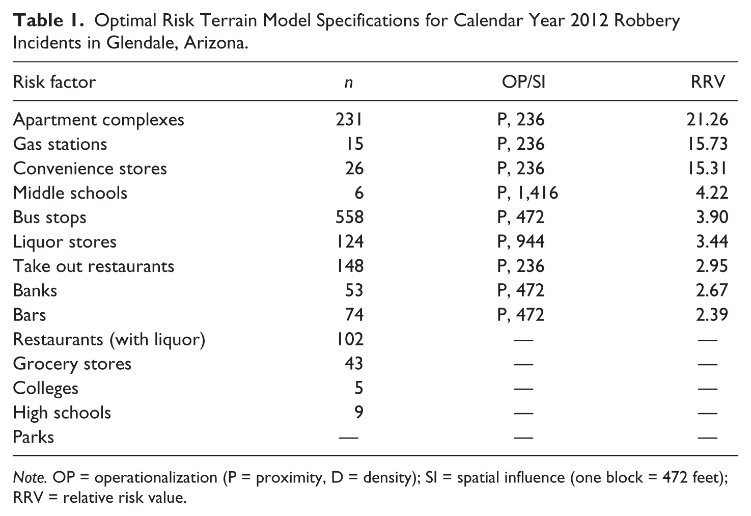
Note. OP = operationalization (P = proximity, D = density); SI = spatial influence (one block = 472 feet); RRV = relative risk value.

Table 1 also presents each risk factor’s relative risk value (RRV),⁵ which represents the weight of influence for each factor relative to one another. For example, a place influenced by convenience stores has an expected rate of robbery that is about 5 times higher than a place influenced by take-out restaurants (RRVs: 15.31 / 2.95 = 5.19). The most problematic risk factor for robbery is apartment complexes; that is, being within proximity of 236 feet (i.e., half a block) of apartment complexes increases the risk of being robbed by a factor of 21.26, relative to places absent any risk factors’ spatial influence. Accordingly, all places may pose a risk of robbery in Glendale, but because of the spatial influence of certain features of the landscape, some places are riskier than others.

Conjunctive Analysis

Crime vulnerability is higher at places influenced by criminogenic features of the environment and increases as these features collocate. RTM identifies these environmental features and the resulting places that are highly vulnerable to illegal behavior. However, additional tools are required to explore specific combinations, or interactions, of risk factors’ spatial influences and their relative effects on crime. For this purpose, we use CACC. Because CACC is described in detail by another author in this issue (see Hart, Rennison, & Miethe, 2017), it is only discussed here within the context of the current approach.

The first step was to prepare the RTM outputs for the conjunctive analysis. This involved coding the spatial influence of each risk factor as a dichotomous variable representing the presence (1) or absence (0) at each micro place (i.e., 236 × 236 raster cell) in Glendale. This resulted in a set of nine standardized raster grids that were spatially joined together to produce a final grid (n = 31,034). Robbery counts for each cell were also joined to this grid (n = 576).⁶ The final data set was imported into SPSS 22 (Statistical Packages for the Social Sciences) to perform a conjunctive analysis using the following code provided by Miethe et al. (2008):

AGGREGATE

/OUTFILE = ’CA_Matrix_file’

/BREAK = A B C D

/Crime = SUM

/N_Cases = N

This produced a data matrix displaying all possible configurations of the aggregated compilation of risk factors’ spatial influences (i.e., behavior settings). Miethe et al. (2008) explained that, “conjunctive analysis involves visual representations of case configurations that convey important information about their nature, diversity, and distribution” (p. 229).

Results of the Conjunctive Analysis

Given nine binary independent variables, the total number of possible case configurations was 512 (2⁹ = 512), of which 61 configurations were observed at least once in Glendale. Miethe et al. (2008) explained that it is important to establish rules about minimum cell frequencies in CACC to accurately interpret patterns of case concentration. Following their lead, we considered case configurations to be dominant if they were observed at least 10 times.⁷ There were 25 dominant case configurations, which are displayed in Table 2, the CACC data matrix. Each row represents a distinct, dominant, case configuration with a unique set of attributes. These attributes reflect the presence (1) or absence (0) of risk factors’ spatial influences as part of each case configuration. Collectively, the particular attributes in each row can be conceptualized as a unique behavior setting for robbery in Glendale (case configuration and behavior setting are used here interchangeably). For example, Case Configuration 6 is characterized by the presence of spatial influences of bus stops and liquor stores and the absence of the spatial influences of apartment complexes, gas stations, convenience stores, middle schools, take-out restaurants, banks, and bars. There were 719 observed instances (i.e., cells) of Case Configuration 6, which represented 2.32% of the study setting. Case Configuration 6 was responsible for 26.90% (n = 155) of robbery incidents, the largest raw share of robberies that occurred in Glendale in 2012.

Table 2.

Conjunctive Analysis Data Matrix of Dominant Case Configurations for Calendar Year 2012 Robbery Risk Factors in Glendale, Arizona.

Case configuration	Apartment complexes	Gas stations	Convenience stores	Middle schools	Bus stops	Liquor stores	Take out restaurants	Banks	Bars	Crime count	Percent crime	Cell count	Percent area	Relative frequency of crime
1	0	0	1	0	1	1	0	0	0	8	1.39	10	0.03	80
2	0	0	0	0	1	1	0	1	1	13	2.26	25	0.08	52
3	0	0	0	0	1	1	0	0	1	22	3.82	96	0.31	22.92
4	0	0	0	0	1	1	0	1	0	21	3.65	92	0.30	22.83
5	1	0	0	0	0	1	0	0	0	9	1.56	41	0.13	21.95
6	0	0	0	0	1	1	0	0	0	155	26.91	719	2.32	21.56
7	0	0	0	0	1	1	1	0	0	3	0.52	17	0.05	17.65
8	0	0	0	0	1	0	0	1	0	6	1.04	40	0.13	15
Mean RFC										237	41.15	1,040	3.35	—
9	0	0	0	0	0	1	0	1	1	2	0.35	16	0.05	12.5
10	1	0	0	0	1	0	0	0	0	3	0.52	26	0.08	11.54
11	0	0	0	0	1	1	1	0	1	1	0.17	12	0.04	8.33
12	0	0	0	0	0	0	1	0	0	1	0.17	14	0.05	7.14
13	0	0	0	0	0	1	0	1	0	4	0.69	58	0.19	6.9
14	0	0	0	0	0	1	1	0	0	1	0.17	17	0.05	5.88
15	0	0	0	0	0	0	0	0	1	9	1.56	173	0.56	5.2
16	0	0	0	0	1	0	0	0	1	3	0.52	66	0.21	4.55
17	0	0	0	0	0	1	0	0	0	85	14.76	2,007	6.47	4.24
18	0	0	0	0	1	0	0	0	0	57	9.90	1,608	5.18	3.54
19	0	0	0	1	0	0	0	0	0	15	2.60	537	1.73	2.79
20	1	0	0	0	0	0	0	0	0	2	0.35	82	0.26	2.44
21	0	0	0	0	0	1	0	0	1	2	0.35	88	0.28	2.27
22	0	0	0	0	0	0	0	1	0	1	0.17	47	0.15	2.13
23	0	0	0	0	0	0	0	0	0	139	24.13	25,091	80.85	0.55
24	0	0	0	1	0	1	0	0	0	0	0.00	33	0.11	0
25	1	0	0	0	1	1	0	0	0	0	0.00	20	0.06	0

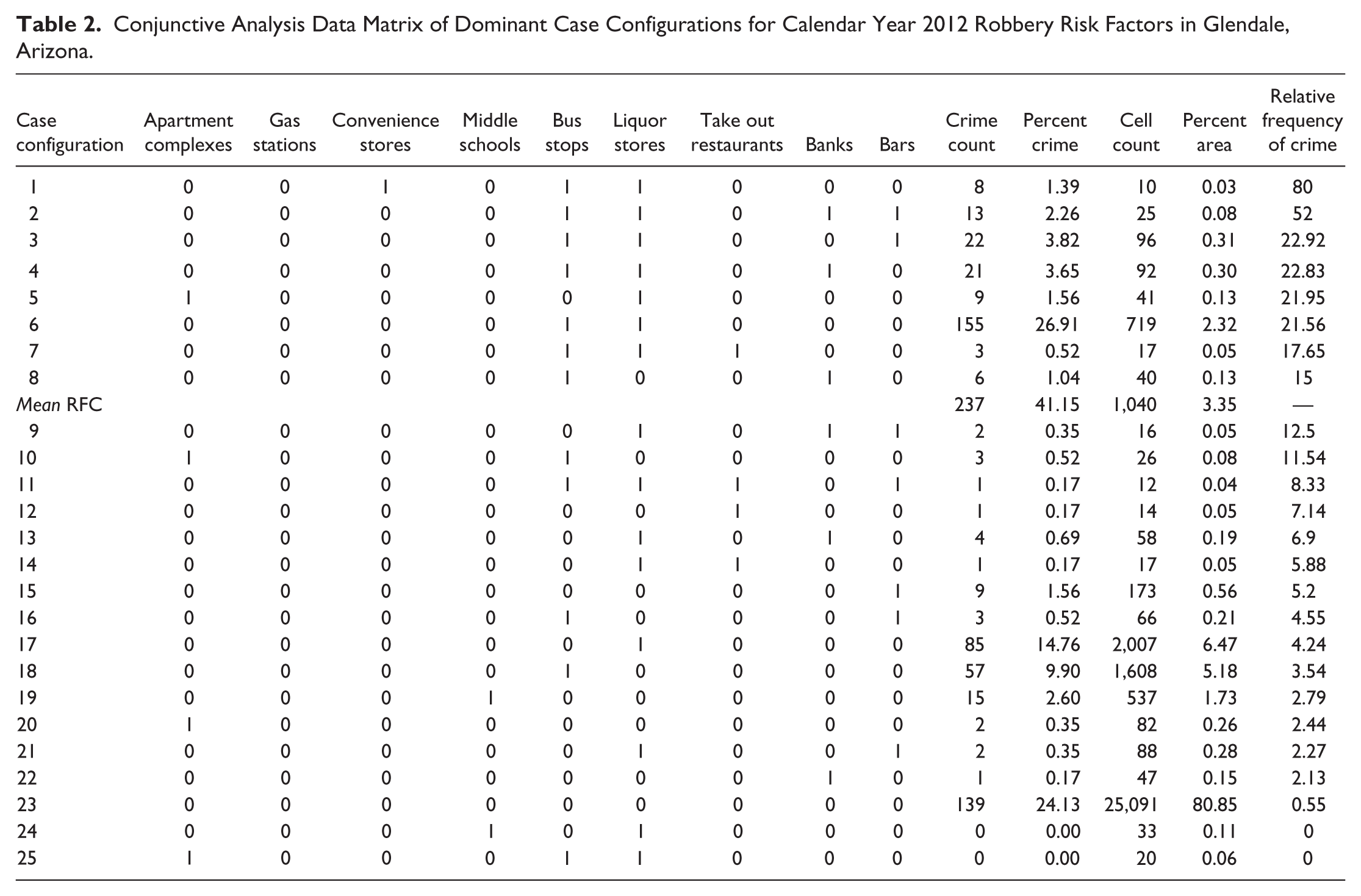
Certain configurations were observed more frequently than others and, as such, were more likely to experience robbery given their larger geographic area. To control for this, the relative frequency of crime (RFC) was calculated as a proportion of robbery incidents per the number of times that behavior setting was observed (i.e., cell count). Dominant case configurations in Table 2 are sorted from highest RFC (Case Configuration 1) to lowest RFC (Case Configuration 25). The RFC of Case Configuration 1 is 80, which makes it the most problematic of the dominant case configurations with regard to the rate of robbery per area.⁸ It is characterized by the spatial influences of convenience stores, bus stops, and liquor stores.

Table 2 also denotes eight dominant case configurations with an above average RFC. It appears that these dominant case configurations above the mean RFC are very often influenced by bus stops and liquor stores. For example, the spatial influence of bus stops is present in all dominant case configurations above the mean RFC, with the exception of Case Configuration 5. Similarly, the spatial influence of liquor stores is in all dominant case configurations above the mean RFC, with the exception of Case Configuration 8. Bus stops and liquor stores appear to be “aggravating” risks of robbery, in that when they interact with other features of the landscape, robbery is most likely, compared with when their spatial influences are absent.

The dominant case configurations with above average RFC are visually represented in Figure 1. Collectively, these eight case configurations were observed 1,040 times, which represents about 3.35% of the entire study setting. However, these case configurations were responsible for 41.15% (n = 237) of robbery incidents in 2012. When considering all dominant behavior settings (with the exception of Case Configuration 23, which was absent the spatial influence of any risk factors), 73.44% of crimes were captured within 18.83% of the entire study area. Thus, few behavior settings—that is, the spatial interactions of specific significant risk factors identified by the risk terrain model—represented a small portion of Glendale’s overall geography but accounted for a substantial share of robbery incident locations. Figure 1 also identifies behavior settings that intersected with robbery hot spots, as determined by kernel density estimation (Hart & Zandbergen, 2014). Overall, nearly two in three behavior settings were also considered hot spots for robbery. Although one in three behavior settings did not directly intersect with a hot spot, Figure 1 shows that many bordered or were otherwise spatially near robbery hot spots.⁹

Figure 1.

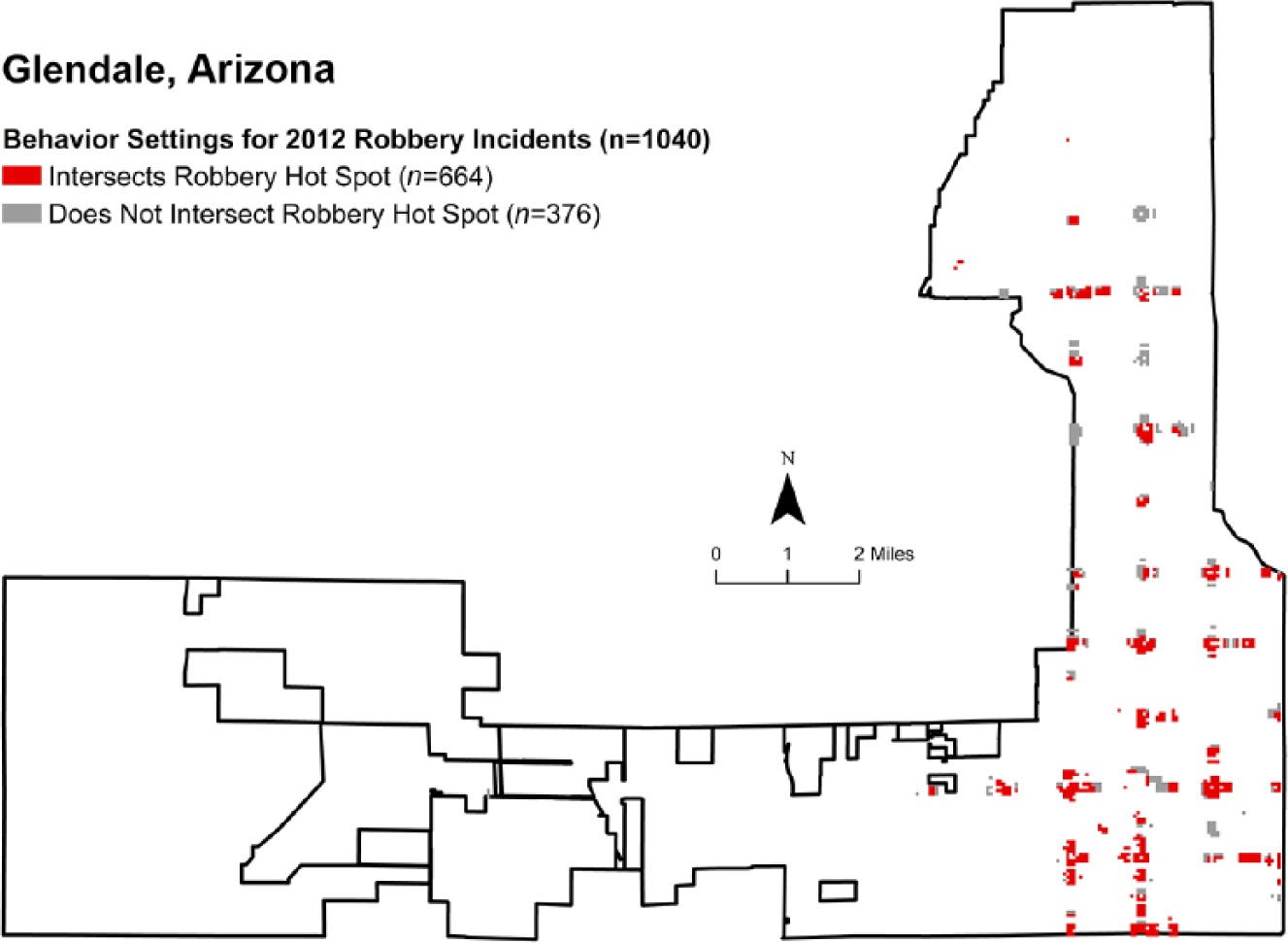
Behavior settings for calendar year 2012 robbery in Glendale, Arizona.

Discussion

We demonstrated how CACC can be used with RTM to explore interactions of risk factors’ spatial influences at places and their relative effects on robbery occurrence. Upon testing 14 environmental features in a risk terrain model, we identified nine significant risk factors for robbery. Given these risk factors, there were 512 possible combinations of risk factors’ spatial influences, or unique behavior settings for robbery, in Glendale, Arizona. Using CACC, we determined that 61 unique behavior settings were present throughout Glendale, and we highlighted 25 dominant behavior settings. The behavior setting that accounted for the largest raw number of robbery incidents was characterized by the presence of two risk factors’ spatial influences: bus stops and liquor stores (i.e., Case Configuration 6). The combined spatial influence of bus stops, liquor stores, and convenience stores constituted the most influential behavior setting (i.e., Case Configuration 1). For example, although Case Configuration 6 accounted for 26.91% of robbery incidents, it was observed a total of 719 times throughout Glendale. On the contrary, Case Configuration 1 was observed 10 times and accounted for 1.39% of robbery incidents. The RFC was computed to account for differences in the geographic area of each behavior setting. When comparing the RFC, it is clear that Case Configuration 1 exerted nearly 4 times the spatial influence of Case Configuration 6. The data matrix produced by the CACC provides a visual tool that highlights the collocation of risk factors’ spatial influences at places throughout a particular environment, which results in unique behavior settings that have varying implications for illegal behavior.

These behavior settings can be mapped in a GIS for analytic purposes or resource allocation. Effective and efficient resource deployment involves maximizing crime prevention through a focus on the smallest number of targets, and the results of this study suggest that police can utilize the information produced by the current methods to great benefit. For example, by focusing on all dominant behavior settings, the GPD would be required to concern themselves with less than one fifth of their entire jurisdiction to address three fourths of their robbery incidents. Moreover, by focusing on dominant behavior settings with above average RFC, the GPD would need to target just 3.35% of places to address more than 41% of robbery incidents. This is demonstrated visually in Figure 1, which displays the dominant behavior settings with above average RFC. The GPD could focus their resources and efforts at the few criminogenic behavior settings shown in Figure 1 to address a substantial share of robbery incidents, an approach that is supported by a large and growing body of literature (Braga, Papachristos, & Hureau, 2014; Kennedy, Caplan, & Piza, 2015). The GPD could address behavior settings that are vulnerable for robbery without removing resources from the places that are already exposed to robbery hot spots. In fact, by targeting behavior settings that are exposed to robbery, and also nearby vulnerable behavior settings, police may be able to effectively guard against spatial displacement because the vulnerable locations are likely the logical next location to carry out an offense. Although research suggests that geographic displacement is often not the result of successful place-based policing efforts (Bowers, Johnson, Guerette, Summers, & Poynton, 2011; Guerette & Bowers, 2009), it is far from nonexistent and can be a threat when a target area is surrounded by nearby criminogenic environments (see Piza & O’Hara, 2014). Therefore, the identification of at-risk behavior settings adjacent to hot spots can heighten crime prevention efforts of the police. Such an approach also accounts for the natural tendency of police officers to stray from their assigned hot spots into adjacent areas in an attempt to disrupt additional street-level crime opportunities (Sorg, Wood, Groff, & Ratcliffe, 2016). Police commanders can allow such activities in hot spots surrounded by at-risk behavior settings, whereas officer discretion can be curtailed more readily at hot spots absent any adjacent at-risk places.

An additional benefit of the current methods is that they provide important insights about the components of criminogenic behavior settings. Specifically, RTM diagnosed environmental risk factors for robbery, and CACC determined where those risk factors’ spatial influences interacted to create ideal contexts for offending. In addition, the CACC enabled a better understanding of the interrelationships between risk factors and how they worked together to yield varying levels of crime. One possible result of these interactions are “risky facilities,” or a small number of facilities, such as bars, within a larger group of those same environmental features that account for a majority of crimes experienced by the entire group of features (Eck, Clarke, & Guerette, 2007). According to Eck et al. (2007), the causes of risky facilities are varied and include such things as the attractiveness of targets or quantity of offenders that visit those facilities or the quality and degree of place management proffered by individuals who are responsible for the well-being of the facilities. This concept is important here because the current methods suggest how different types of features may interact with one another to produce the conditions that make specific facilities within those larger groups of features problematic. Thus, even within groups of risk factors, certain risky facilities may emerge given the presence of other qualities in their surrounding context.

This information could help police to prioritize the risk factors and, moreover, the specific facilities within those broader groups of risk factors that should be addressed. For example, the CACC suggested that bus stops and liquor stores often interacted with other risk factors to aggravate robbery occurrence, but knowing the dynamics among these and other risk factors at places can help police to further determine the particular facilities within these groups of features that come together and create criminogenic behavior settings that require intervention. This is illustrated, for example, when comparing Case Configurations 4 and 9. Both configurations are similar to the extent that they are influenced by three risk factors, and that both configurations are influenced by banks and liquor stores. However, whereas Configuration 4 is also influenced by bus stops, Configuration 9 is also influenced by bars. Although these configurations vary with regard to just one risk factor, Case Configuration 4 has nearly twice the RFC as Case Configuration 9. Moreover, Case Configuration 4 experienced more than 10 times the number of robbery incidents than Case Configuration 9. Furthermore, not all bus stops or bars should be treated equally; those next to banks and/or liquor stores present a nuanced and heightened risk compared with other similar entities. From a practical perspective, CACC highlights important risk factor interactions, allowing police to make better decisions regarding the most effective allocation of resources to address the most influential behavior settings, and risk factors within them, and to therefore achieve the greatest reductions in crime. The current methods can also aid in the development of police practices that are tailored to each place’s unique environmental dynamics. More specifically, RTM and CACC contribute to a better understanding of each location’s unique environmental context and the ways in which the spatial influence of criminogenic environmental features effectively create behavior settings for illegal behavior. RTM identifies environmental risk factors, and CACC enables the assessment of the relative combination of risk factors’ spatial influences and their differential effects on crime at places. Identifying the dynamics among environmental features and their particular crime outcomes helps to develop a sense of what to expect at different places and informs approaches to policing that are place-based and focused on altering the conditions across the environmental landscape that create opportunities for crime.

RTM and CACC could be integrated into the existing administrative structures of police agencies to allow for ongoing assessments and evaluations of various police activities that are intended to reduce and prevent crime. For example, criminogenic behavior settings can be identified, and specific police responses can be deployed to the most problematic settings to address the spatial influences of criminogenic environmental features. Crime occurrence at these behavior settings can be examined at future time periods to determine whether crime prevention was achieved. Moreover, different locations that are otherwise considered a behavior settings of the same type can be compared with regard to the particular type of response they received (if any at all) to determine what works, what works best, and what is ineffective in preventing crime at very specific settings, that is, perhaps allowing for a scalpel rather than axe approach to place-based policing. Based on these evaluations, interventions can be updated and redeployed so that ineffective responses are rejected and the most effective strategies, at specific behavior settings, are retained. The goal is a systematic approach to policing that culminates in a “playbook” of strategies that are known to work in addressing the dynamics among features of the environment that create conditions that are conducive to crime.

Conclusion

RTM is a crime analysis tool that guides place-based approaches to policing through theoretically grounded empirical analysis that diagnoses environmental risk factors for crime and determines the places where their spatial influences are collocated to produce vulnerability for illegal behavior. However, the collocation of certain risk factors’ spatial influences may result in more crimes than the collocation of a different set of risk factors’ spatial influences. Absent from existing RTM outputs and methods is a straightforward method to compare these relative interactions and their effects on crime. However, CACC can enable such assessments. As a multivariate method for the analysis of discrete categorical data, it can describe the interrelationships between the spatial influence of risk factors and their varying effects on crime occurrence. Therefore, we incorporated the outputs of a risk terrain model into a CACC to explore the dynamics among certain risk factors’ spatial influences and how they create unique environmental contexts, or behavior settings, for crime across microlevel places. We demonstrated that most crime takes place within a few dominant behavior settings that cover a small geographic area and, further, that some behavior settings were more influential on crime than others. Moreover, we identified particular environmental risk factors that aggravated the influence of other risk factors. By focusing on these microlevel environmental crime contexts, police can more efficiently target their resources. In addition, the methods in the current study could be used to further enhance place-based approaches to policing that fundamentally address the dynamics among environmental features that produce opportunities for crime.

Footnotes

Authors’ Note

The views presented as those of the authors and do not necessarily represent the position of the National Institute of Justice.

Declaration of Conflicting Interests

The author(s) declared no potential conflicts of interest with respect to the research, authorship, and/or publication of this article.

Funding

The author(s) disclosed receipt of the following financial support for the research, authorship, and/or publication of this article: This research was supported in part by a grant from the National Institute of Justice (Award #2013-IJ-CX-0053).

Notes

Author Biographies

Joel M. Caplan is associate professor at Rutgers University School of Criminal Justice and Deputy Director of the Rutgers Center on Public Security. He earned a PhD in social welfare policy from the University of Pennsylvania and has professional experiences as a police officer, 9-1-1 dispatcher, and emergency medical technician, which give him a unique and practical research perspective. He specializes in applying geospatial technology to actionable scholarship and is currently leading cutting-edge research on policing, crime control, and risk management, while he advises agencies in the United States and around the world on matters of public safety and security.

Leslie W. Kennedy is currently university professor of criminal justice at Rutgers University and director of the Rutgers Center on Public Security. In his most recent research, he extends his interest in risk assessment, focusing on crime mapping and the development (with Joel Caplan) of risk terrain modeling (RTM) for use by police in preventing crime. He has published in major journals in criminology and criminal justice, including Criminology, Justice Quarterly, and Journal of Quantitative Criminology.

Jeremy D. Barnum is a doctoral student at School of Criminal Justice, Rutgers University–Newark, and a project manager in the Rutgers Center on Public Security. His research interests include geographic information science and spatial analysis, policing, and crime prevention.

Eric L. Piza is an associate professor at John Jay College of Criminal Justice, City University of New York. His research focuses on the spatial analysis of crime patterns, crime control technology, and the integration of academic research and police practice. His scholarship has appeared in outlets, including Criminology, Journal of Experimental Criminology, Journal of Research in Crime and Delinquency, Journal of Quantitative Criminology, and Justice Quarterly.

References

Barker

R. G.

(1968). Ecological psychology: Concepts and methods for studying the environment of human behavior. Stanford, CA: Stanford University Press.

Barker

R. G.

Wright

H. F.

(1951). One boy’s day: A specimen record of behavior. New York, NY: Harper & Row.

Barnum

J. D.

Caplan

J. M.

Kennedy

L. W.

Piza

E. L.

(2016). The crime kaleidoscope: A cross-jurisdictional analysis of place features and crime in three urban environments. Applied Geography. Advance online publication. doi: 10.1016/j.apgeog.2016.12.011.

Bernasco

Block

(2009). Where offenders choose to attack: A discrete choice model of robberies in Chicago. Criminology, 47, 93-130.

Bernasco

Block

(2011). Robberies in Chicago: A block-level analysis of the influence of crime generators, crime attractors, and offender anchor points. Journal of Research in Crime & Delinquency, 48, 33-57.

Bernasco

Bruinsma

G. J.

Pauwels

L. J.

Weerman

F. M.

(2013). Adolescent delinquency and diversity in behavior settings. Australian & New Zealand Journal of Criminology, 46, 357-378.

Bowers

Johnson

Guerette

Summers

Poynton

(2011). Spatial displacement and diffusion of benefits among geographically focused policing initiatives: A meta-analytical review. Journal of Experimental Criminology, 7, 347-374.

Braga

A. A.

Hureau

D. M.

Papachristos

A. V.

(2011). The relevance of micro places to citywide robbery trends: A Longitudinal analysis of robbery incidents at street corners and block faces in Boston. Journal of Research in Crime & Delinquency, 48, 7-32.

Braga

A. A.

Papachristos

A. V.

Hureau

D. M.

(2014). The effects of hot spots policing on crime: An updated systematic review and meta-analysis. Justice Quarterly, 31, 633-663.

10.

Brantingham

(1995). Criminality of place: Crime generators and crime attractors. European Journal on Criminal Policy and Research, 3, 5-26.

11.

Caplan

J. M.

(2011). Mapping the spatial influence of crime correlates: A comparison of operationalization schemes and implications for crime analysis and criminal justice practice. Cityscape, 13, 57-83.

12.

Caplan

J. M.

Kennedy

L. W.

(2016). Risk Terrain Modeling: Crime prediction and risk reduction. Oakland: University of California Press.

13.

Caplan

J. M.

Kennedy

L. W.

Miller

(2011). Risk terrain modeling: Brokering criminological theory and GIS methods for crime forecasting. Justice Quarterly, 28, 360-381.

14.

Caplan

J. M.

Kennedy

L. W.

Piza

E. L.

(2013). Risk Terrain Modeling Diagnostics Utility user manual (Version 1.0). Newark, NJ: Rutgers Center on Public Security.

15.

Drawve

Thomas

S. A.

Walker

J. T.

(2016). Bringing the physical environment back into neighborhood research: The utility of RTM for developing an aggregate neighborhood risk of crime measure. Journal of Criminal Justice, 44, 21-29.

16.

Eck

J. E.

Clarke

R. V.

Guerette

R. T.

(2007). Risky facilities: Crime concentration in homogeneous sets of establishments and facilities. Crime Prevention Studies, 21, 225-264.

17.

Federal Bureau of Investigation. (2013). Robbery. In Crime in the United States, 2012. Washington, DC: U.S. Department of Justice.

18.

Groff

E. R.

(2015). Informal social control and crime events. Journal of Contemporary Criminal Justice, 31, 90-106.

19.

Groff

E. R.

Lockwood

(2014). Criminogenic facilities and crime across street segments in Philadelphia: Uncovering evidence about the spatial extent of facility influence. Journal of Research in Crime & Delinquency, 51, 277-314.

20.

Guerette

Bowers

(2009). Assessing the extent of crime displacement and diffusion of benefits: A review of situational crime prevention evaluations. Criminology, 47, 1331-1368.

21.

Hart

T. C.

Miethe

T. D.

(2009). Self-defensive gun use by crime victims: A conjunctive analysis of its situational contexts. Journal of Contemporary Criminal Justice, 25, 6-19.

22.

Hart

T. C.

Miethe

T. D.

(2014). Street robbery and public bus stops: A case study of activity nodes and situational risk. Security Journal, 27, 180-193.

23.

Hart

T. C.

Miethe

T. D.

(2015). Configural behavior settings of crime event locations: Toward an alternative conceptualization of criminogenic microenvironments. Journal of Research in Crime & Delinquency, 52, 373-402.

24.

Hart

T. C.

Rennison

C. M.

Miethe

T. D.

(2017). Identifying patterns of situational clustering and contextual variability in criminological data: An overview of conjunctive analysis of case configurations. Journal of Contemporary Criminal Justice, 33, 112-120.

25.

Hart

T. C.

Zandbergen

P. A.

(2014). Kernel density estimation and hotspot mapping: Examining the influence of interpolation method, grid cell size, and bandwidth on crime forecasting. Policing: An International Journal of Police Strategies & Management, 37, 305-323.

26.

Heffner

(2013). Statistics of the RTMDx Utility. In Caplan

J. M.

Kennedy

L. W.

Piza

E. L.

(Eds.), Risk terrain modeling diagnostics utility user manual, Version 1.0 (pp. 35-39). Newark, NJ: Rutgers Center on Public Security.

27.

Kennedy

L. W.

Caplan

J. M.

Piza

E. L.

(2011). Risk clusters, hotspots, and spatial intelligence: Risk terrain modeling as an algorithm for police resource allocation strategies. Journal of Quantitative Criminology, 27, 339-362.

28.

Kennedy

L. W.

Caplan

J. M.

Piza

E. L.

(2015). A multi-jurisdictional test of risk terrain modeling and place-based evaluation of environmental risk-based patrol deployment strategies. Newark, NJ: Rutgers Center on Public Security.

29.

Kennedy

L. W.

Caplan

J. M.

Piza

E. L.

Buccine-Schraeder

(2016). Vulnerability and exposure to crime: Applying risk terrain modeling to the study of assault in Chicago. Applied Spatial Analysis and Policy, 9, 529-548.

30.

McGloin

J. M.

Sullivan

C. J.

Kennedy

L. W.

(2012). When crime appears: The role of emergence. New York, NY: Routledge.

31.

Miethe

T. D.

Hart

T. C.

Regoeczi

W. C.

(2008). The conjunctive analysis of case configurations: An exploratory method for discrete multivariate analyses of crime data. Journal of Quantitative Criminology, 24, 227-241.

32.

Piza

Feng

Kennedy

Caplan

(2016). Place-based correlates of motor vehicle theft and recovery: Measuring spatial influence across neighborhood context. Urban Studies. Advance online publication. doi:10.1177/0042098016664299

33.

Piza

O’Hara

(2014). Saturation foot-patrol in a high-violence area: A quasi-experimental evaluation. Justice Quarterly, 31, 693-718.

34.

Popov

Chopalov

(2012). Crossing over: The interdisciplinary meaning of behavior setting theory. International Journal of Humanities and Social Science, 2, 18-27.

35.

Rice

K. J.

Smith

W. R.

(2002). Socioecological models of automotive theft: Integrating routine activity and social disorganization approaches. Journal of Research in Crime & Delinquency, 39, 304-336.

36.

Roncek

D. W.

Bell

(1981). Bars, blocks, and crimes. Journal of Environmental Systems, 11, 35-47.

37.

Roncek

D. W.

Faggiani

(1985). High schools and crime: A replication. The Sociological Quarterly, 26, 491-505.

38.

Roncek

D. W.

Maier

P. A.

(1991). Bars, blocks, and crimes revisited: Linking the theory of routine activities to the empiricism of “hot spots.” Criminology, 29, 725-753.

39.

Sampson

R. J.

Groves

W. B.

(1989). Community structure and crime: Testing social-disorganization theory. American Journal of Sociology, 94, 774-802.

40.

Schoggen

(1989). Behavior settings: A revision and extension of Roger G. Barker’s ecological psychology. Stanford, CA: Stanford University Press.

41.

Shaw

C. R.

McKay

H. D.

(1942). Juvenile delinquency in urban areas. Chicago, IL: University of Chicago Press.

42.

Sherman

L. W.

(1995). Hot spots of crime and criminal careers of places. In Eck

J. E.

Weisburd

(Eds.), Crime and place: Crime prevention studies (pp. 13-52). Monsey, NY: Criminal Justice Press.

43.

Sherman

L. W.

Gartin

P. R.

Buerger

M. E.

(1989). Hot spots of predatory crime: Routine activities and the criminology of place. Criminology, 27, 27-56.

44.

Shevky

Bell

(1955). Social area analysis: Theory, illustrative application, and computational procedures. Stanford, CA: Stanford University Press.

45.

Smith

W. R.

Frazee

S. G.

Davison

E. L.

(2000). Furthering the integration of routine activity and social disorganization theories: Small units of analysis and the study of street robbery as a diffusion process. Criminology, 38, 489-524.

46.

Sorg

Wood

Groff

Ratcliffe

(2016). Explaining dosage diffusion during hot spot patrols: An application of optimal foraging theory to police officer behavior. Justice Quarterly. Advance online publication. doi:10.1080/07418825.2016.1244286

47.

St. Jean

P. K. B.

(2007). Pockets of crime: Broken windows, collective efficacy, and the criminal point of view. Chicago, IL: University of Chicago Press.

48.

Taylor

R. B.

(1997). Social order and disorder of street-blocks and neighborhood: Ecology, microecology and the systemic model of social disorganization. Journal of Research in Crime & Delinquency, 34, 113-155.

49.

Wicker

A. W.

(1979). An introduction to ecological psychology. Monterey, CA: Brooks Cole.

50.

Wright

R. T.

Decker

S. H.

(1997). Armed robbers in action: Stickups and street culture. Lebanon, NH: Northeastern University Press.