On the performance of a dual-mode non-linear vibration energy harvesting device

Abstract

The research trend for harvesting energy from the ambient vibration sources has moved from using a linear resonant generator to a non-linear generator in order to improve on the performance of a linear generator; for example, the relatively small bandwidth, intolerance to mistune and the suitability of the device for low-frequency applications. This article presents experimental results to illustrate the dynamic behaviour of a dual-mode non-linear energy-harvesting device operating in hardening and bi-stable modes under harmonic excitation. The device is able to change from one mode to another by altering the negative magnetic stiffness by adjusting the separation gap between the magnets and the iron core. Results for the device operating in both modes are presented. They show that there is a larger bandwidth for the device operating in the hardening mode compared to the equivalent linear device. However, the maximum power transfer theory is less applicable for the hardening mode due to occurrence of the maximum power at different frequencies, which depends on the non-linearity and the damping in the system. The results for the bi-stable mode show that the device is insensitive to a range of excitation frequencies depending upon the input level, damping and non-linearity.

Keywords

non-linear energy harvesting hardening bi-stable Duffing oscillator

Introduction

Harvesting energy from ambient sources has become an area of increasing interest within the last decade. Among the sources, ambient vibration has been considered as a potential source to power wireless sensors in remote and hostile environments.

Vibration-based energy-harvesting devices are often modelled mechanically as a base-excited linear single-degree-of-freedom mass–spring–damper system. In this case, the maximum power that can be harvested occurs when the device is excited at its natural frequency (Williams and Yates, 1996). However, the ambient frequency may not be tonal and could vary with time, which can degrade the performance of the device drastically. To overcome this limitation, ways have been suggested to alter the natural frequency of the device, so that it tracks the ambient frequency either actively or passively (Tang et al., 2010; Zhu et al., 2010). The power that can be harvested by such a device is, however, small and the tuning schemes are complex. Thus, passive tuning is often more desirable than the active tuning due to power requirements. Cammarano et al. (2010), on the other hand, improved the bandwidth of a linear resonant generator by modifying the reactive component of the electrical load impedance.

Low-frequency applications are also another challenge for the linear devices, since for a given excitation displacement, power harvested is proportional to the cube of the ambient frequency (Williams and Yates, 1996). To overcome this, Külah and Najafi (2008) suggested a method to convert a low ambient frequency to a much higher frequency. Using another approach, Bowers and Arnold (2009) studied a non-resonant device consisting of a magnetic ball with no spring element. When excited, the ball moves freely in a spherical enclosure which has a copper coil wrapped around it to capture the energy from low ambient frequency such as human walking.

An alternative approach is to use stiffness non-linearity to overcome the sensitivity due to mistuning and poor performance at low frequency. The most common configuration consists of a cubic stiffness in addition to a linear stiffness, which together with the inertial mass forms a Duffing oscillator. The Duffing oscillator can be further divided into three common modes of operation, which are called hardening, bi-stable and softening. The first two modes are used most frequently in the design of an energy harvester.

The theoretical studies on the hardening mode have been conducted by Ramlan et al. (2010) and Quinn et al. (2011) and the experimental studies by Mann and Sims (2009) and Barton et al. (2010). Because it generally has a broader bandwidth than a linear system, a tuning mechanism embedded in the device to broaden the frequency range is not necessary.

The bi-stable mode of operation has also been widely studied, including theoretical work (Litak et al., 2010; McInnes et al., 2008; Ramlan et al., 2008) and experimental work (Andò et al., 2010; Arrieta et al., 2010; Cammarano et al., 2011; Erturk and Inman, 2011; Mann and Owens, 2010; Stanton et al., 2010). This device is particularly useful at low frequency. A negative stiffness is used in conjunction with a linear positive stiffness to convert the low frequency ambient motion to a much higher frequency motion.

This article presents experimental results on the dual-mode non-linear energy harvesting device which has the capability to operate in both the hardening mode and the bi-stable mode by simply adjusting the distance between a set of magnets and an iron core. The results on the dynamic response of the device operating in both modes are presented. The particular device presented in this article show that, in its two modes, it demonstrates two ways of increasing the bandwidth. The results on the power harvested by the device involving both modes are also presented.

The content of the article is organized as follows. The next section describes the equation of motion that represents the Duffing oscillator. This is followed by the experimental investigation section which describes the device and the setup of the experiment which includes both quasi-static and dynamic measurements. The following section presents the experimental results of the hardening mode covering the dynamics and power-harvested aspects of the device which validates the modelling work in the study by Ramlan et al. (2010). This is followed by the section presenting the experimental results of the bi-stable mode which covers both the dynamics and power-harvested aspects of the device. This article is then concluded with some final remarks.

Equation of motion of the non-linear system

The equations of motion for both the hardening and bi-stable systems are given in the study by Ramlan et al. (2010), to which the reader is referred. Accordingly, only a brief description of the theory is given here.

The system of interest consists of a mass connected in series with a parallel combination of a damper and a non-linear spring whose spring force is of the form $k_{1} x + k_{3} x^{3}$ , where $k_{1}$ is the linear spring constant, $k_{3}$ is the non-linear spring constant and $x$ is the displacement of the seismic mass. The equation of motion for a base-excited hardening Duffing oscillator is given by (Kovacic and Brennan, 2011)

m \overset{\cdot\cdot}{z} + c \overset{\cdot}{z} + k_{1} z + k_{3} z^{3} = - m \overset{\cdot\cdot}{y}

(1)

where $z = x - y$ is the relative displacement between the seismic mass $x$ and the base displacement $y$ . If it is assumed that the excitation is harmonic at frequency $ω$ , such that $y = Y \cos (ω t)$ , equation (1) can be expressed in non-dimensional form as

u ″ + 2 ζ u' + u + γ u^{3} = Ω^{2} \cos (Ω τ + ϕ)

(2)

where $ω_{n} = \sqrt{k_{1} / m}$ , $Ω = ω / ω_{n}$ , $u = z / Y$ , $γ = (k_{3} / k_{1}) Y^{2}$ , $τ = ω_{n} t$ , $ζ = c / 2 m ω_{n}$ , $(•)' = d / d τ$ and $ϕ$ is the phase angle between the excitation and the response. The degree of non-linearity of the device $γ$ depends on both the physical properties of the device, $k_{1}$ and $k_{3}$ , and the level of the input displacement, $Y$ . Thus, when the amplitude of excitation is small, the system behaves approximately in a linear manner.

The dynamics of the system described by equation (1) varies depending on the linear stiffness $k_{1}$ and non-linear stiffness $k_{3}$ . When $k_{3} > 0$ , the device acts as a hardening system so that the frequency response curve (FRC) bends to the right. The FRC of the hardening system exhibits jump phenomena. As the frequency is slowly increased from zero, the amplitude of the response first increases and then jumps down to a much smaller value. As the frequency is slowly decreased from a high frequency, the amplitude of the response slowly increases and then jumps up to a larger amplitude before decreasing. The system is in softening mode when $k_{3} < 0$ . In this mode, the FRC bends to the left. The dynamics of the hardening and the softening modes have some similarity at least in terms of the jump characteristics (Brennan et al., 2008).

Another type of non-linear behaviour which can be derived from equation (1) is known as the snap-through or bi-stable mode oscillator. This type of non-linear behaviour is realized by setting $k_{1} < 0$ and $k_{3} > 0$ . The dynamics of such a system is completely different from the hardening and softening modes (Ramlan et al., 2010). The bi-stable mechanism has a double-well potential which is composed of two stable static equilibrium positions and one unstable static equilibrium position. The motion of such a system can be categorized into two distinct types. The first is a local oscillation about one of the two stable equilibrium positions. This occurs when the input is small such that the potential barrier is too large for the mass to snap from one stable equilibrium position to another. The global oscillation is induced when the input is of much larger value such that the oscillation can overcome the potential barrier.

Experimental investigation

Device configuration

Figure 1(a) shows the device used in the experimental work. It consists of two main parts. The first part consists of a beam fixed at one end with a mass and four magnets attached at the other end. The second part is made up of an iron core with a copper coil wrapped around it. Figure 1(b) depicts the arrangement of the magnets on the beam. This arrangement allows the continuous flow of magnetic flux between the magnets and the iron core. As the beam oscillates, a voltage is induced in the coil and energy can be harvested by attaching a suitable electrical circuit.

Figure 1.

Photographs showing the device: (a) full view and (b) the arrangement of the magnets. Device parameters: beam width b = 38.21 mm, beam thickness t = 0.5 mm, length (various beam lengths L = 42.70 and 47.30 mm), Young’s modulus E = 200 GPa, tip mass m = 115 g and gap (various gaps, d = 1.50 mm (hardening mode), d = 0.6 and 0.8 mm (bi-stable mode))

The total stiffness of the system is the combination of the positive stiffness from the beam and the negative stiffness from the magnets resulting in a non-linear stiffness characteristic. The two main parts of the device are separated by a gap $d$ which controls the degree of non-linearity. When the gap is large, the system behaves as a hardening system, and when the gap is small, the system behaves as a bi-stable system. The words ‘large’ and ‘small’ are used for relative comparison between the two systems only. In practice, the total stiffness is very sensitive to the gap $d$ as the system can change from being a hardening system to a bi-stable system when the gap is decreased by only 1 mm. The device behaved as a linear system for a small or moderate deflection when the coil was removed as the stiffness of the system was then due to the stiffness of the beam only. Representative force–deflection curves for linear, hardening and bi-stable systems are plotted in Figure 2 to illustrate the differences between the three systems.

Figure 2.

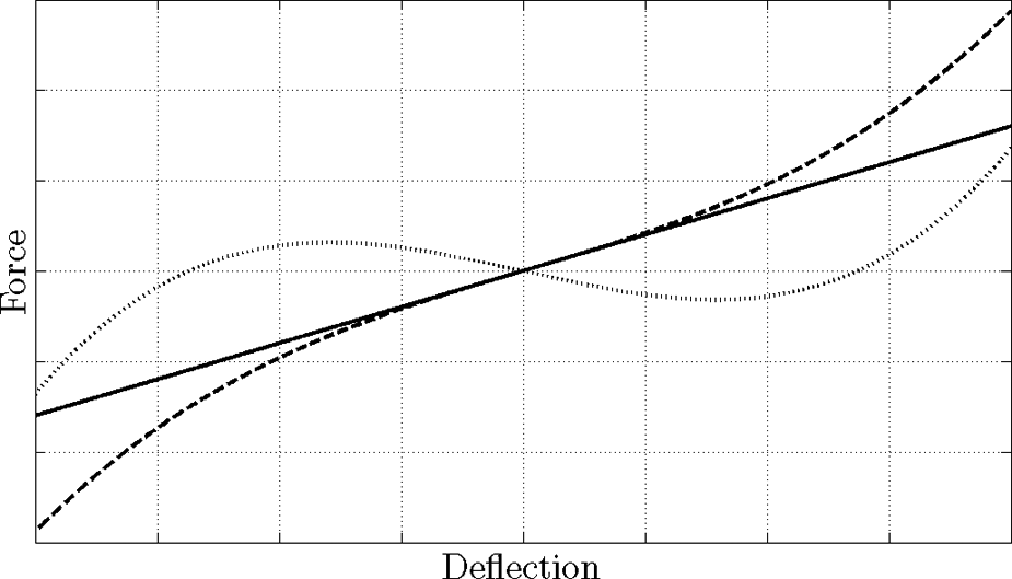
Representative theoretical force–deflection curves: linear (when the coil part is removed) (solid), hardening (when the gap is large) (dashed) and bi-stable (when the gap is small) (dotted).

Some of the studies on this device have been previously published in the studies by Burrow and Clare (2007), Ramlan et al. (2009), Ramlan (2009), Barton et al. (2010), and Cammarano et al. (2011). This article adds to the literature by validating the previously published modelling work on both hardening and bi-stable modes. It also includes the feasibility study on the maximum power transfer theorem on the device operating in the hardening mode.

Experimental setup

The experiment had two parts. The first part was the quasi-static measurement of the deflection of the beam and the restoring force of the beam. The second part was the dynamic measurement of the acceleration of the mass.

In the quasi-static measurement, the stiffness of the system was measured to determine the stiffness characteristic together with the strength of the non-linearity. A force gauge was used to measure the restoring force of the beam as the mass attached to the beam was driven by a shaker with a high amplitude displacement at a very low frequency, that is, 0.5 Hz. The force gauge was connected to the beam using a connecting arm and the deflection of the tip of the beam was measured using a linear variable differential transformer (LVDT).

In the dynamic measurement, the whole device was placed onto a shaker so that the system was base-excited rather than force excited. The frequency was increased from 10 to 40 Hz in 1 Hz steps and then decreased from 40 to 10 Hz with the same frequency increment. Since the system was non-linear, the amplitude of the input displacement had to be kept constant for all frequencies, which was achieved by a feedback controller connected to the shaker.

The damping in the system was altered by changing the external electrical resistance connected to the coil using a resistor box. The electrical damping is inversely proportional to the resistance, so the larger the resistance, the smaller the damping. A PCB accelerometer was used to measure the acceleration of the tip mass, which was recorded together with the input displacement and the voltage across the load resistance at each frequency using a Data Physics signal analyser. The experimental setup for the dynamic measurement is shown in Figure 3.

Figure 3.

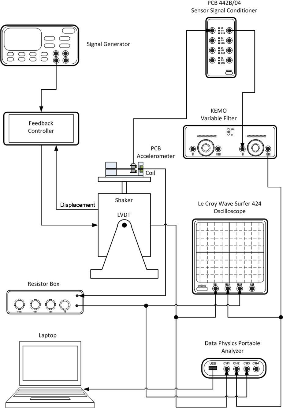
Experimental setup for the dynamic measurements.

Experimental results of the hardening mode

Response of the device with respect to non-linearity and damping

The dynamics of the system were first observed by investigating the response of the system with differing degrees of non-linearity and damping. It can be seen in equation (2) that the non-linearity of the systems depends on the stiffness $k_{1}$ and $k_{3}$ as well as on the amplitude of the input displacement, $Y$ , that is, $γ = \frac{k_{3}}{k_{1}} Y^{2}$ .

Figure 4 shows the fitted curve of the measured force–deflection for two configurations which have different length while the gap $d$ for both cases was maintained at 1.50 mm. The relationship between the force and the deflection for both configurations are, respectively, given by

F (x) \approx 1495 x + 4.26 \times 10^{7} x^{3} for L = 42.70 mm

(3)

F (x) \approx 946 x + 3.30 \times 10^{7} x^{3} for L = 47.30 mm

(4)

Figure 4.

Force–deflection curves for the hardening mode for L = 42.70 mm (solid) and L = 47.30 mm (dashed) with d = 1.50 mm for both configurations.

For these two configurations, the negative stiffness due to the magnets is similar for both cases due to the gap being the same. Thus, the total stiffness is strongly determined by the linear stiffness from the beam given by $k_{beam} = 3 EI / L^{3}$ , where $E$ is the Young’s modulus and $I$ is the second moment of area of the beam, respectively. The linear stiffness increases as the length of the beam decreases, the system with L = 42.70 mm has a larger linear stiffness as well as a larger non-linearity compared to that with L = 47.30 mm. The dynamic responses for both configurations, for an input amplitude of 0.1 mm at each frequency, are shown in Figure 5. It can be seen that the system with a shorter beam jumps up and jumps down at higher frequencies because of the larger linear stiffness and the non-linearity.

Figure 5.

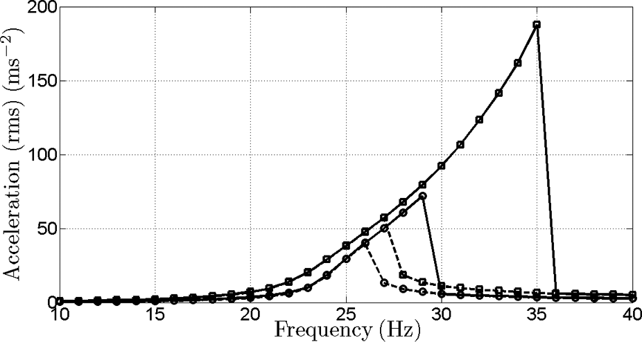
Measured rms acceleration of the mass of the hardening mode with different beam length for the open-circuit system while the gap d = 1.50 mm and the amplitude of the input Y = 0.1 mm are fixed; L= 42.70 mm [sweep-up (――Δ――), sweep-down (──Δ──)] and L = 47.30 mm [sweep-up (――o――), sweep-down (──o──)].

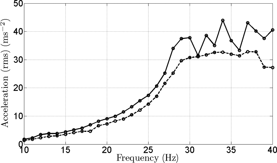
The dependence of the non-linearity on the amplitude of the input displacement was investigated by setting different levels of input displacement, that is, 0.1 and 0.2 mm for each frequency sweep. The measured responses of both configurations are shown in Figure 6. It can be seen that in the configuration with a larger input, the non-linearity has a greater effect, which is shown by the higher jump-up and jump-down frequencies.

Figure 6.

Measured rms acceleration of the mass of the hardening mode with different input level for the open-circuit system while the gap d = 1.50 mm and the length L = 42.70 mm are fixed; Y = 0.1 mm [sweep-up (――o――), sweep-down (── o──)] and Y = 0.2 mm [sweep-up (――――), sweep-down (────)].

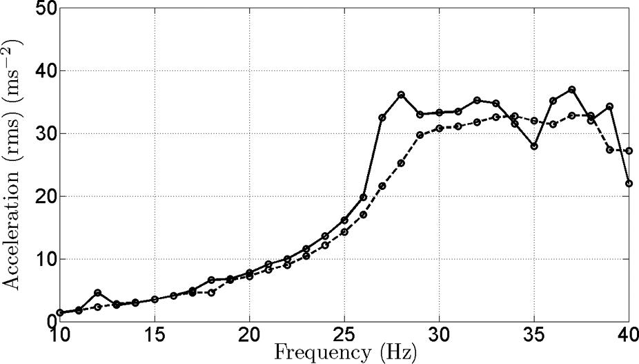
The jump-up frequency depends only on the non-linearity, while the jump-down frequency depends on both the damping and the non-linearity (Brennan et al., 2008; Ramlan et al., 2009). Figure 7 shows the measured response of the open-circuit system and that with a 200 Ω resistance for different configurations. From this figure, it is confirmed that the jump-up frequency for all configurations depends strongly on the non-linearity and not on the damping as the response for each configuration jumps up at the same frequency for both systems. The figure also shows that the jump-down frequency depends on both the damping and the non-linearity. For a given non-linearity, the jump-down frequency is inversely proportional to the damping. In all cases, the jump-down frequency for the open-circuit system is much larger than that with the 200 Ω resistance attached.

Figure 7.

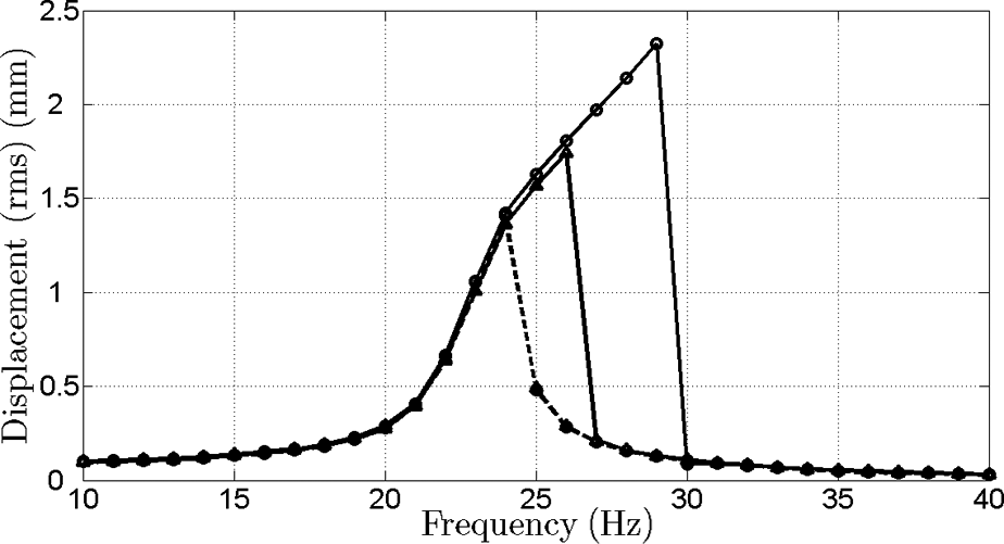
Measured rms displacement response for the open-circuit system [sweep-up (――o――), sweep-down (── o ──)] and 200 Ω load [sweep-up (――Δ――), sweep-down (──Δ──)] for the system with L = 42.70 mm, d = 1.50 mm and Y = 0.1 mm.

Power harvested by a resistive load

The maximum potential power harvested by the hardening mode is now compared to that harvested using the linear mode in this section. The maximum power harvested by the hardening mode is determined by measuring the voltage across the resistance at a frequency of 1 Hz below the jump-down frequency. This is because it is not possible to measure a large steady-state response at the jump-down point since the change in the response, from a larger amplitude to a lower amplitude, is very rapid and the response is only in steady state when it converges to the lower amplitude oscillation.

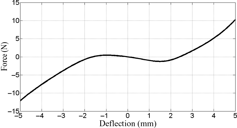
The maximum power harvested by the equivalent linear mechanism could not be measured exactly using the same input as the hardening mechanism. This was because the region in which the device behaves linearly was small and limited to a small input only. For a fair comparison, the linear mechanism was assumed to have the same stiffness as the linear stiffness in the hardening mechanism. This was done by assuming that there is only the linear stiffness component of the hardening mechanism acting across the whole range of the deflection, −5 to 5 mm, as shown by the dashed line in Figure 8. The voltage generated across the resistance is first determined using the transmissibility plot as shown in Figure 9 for a very small random input displacement (e.g. 0.0054 mm (root mean square, rms)), so that the system still operates in the linear region. Since the system is linear, the ratio between the input displacement and the generated voltage is always constant. Thus, the generated voltage due to the same input as applied to the hardening system can be computed using this ratio.

Figure 8.

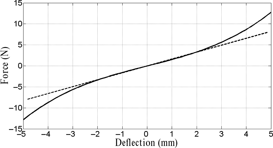
Force–deflection curves for the hardening mode (solid) and the equivalent linear system (dashed) with L = 42.70 mm, d = 1.50 mm and Y = 0.1 mm.

Figure 9.

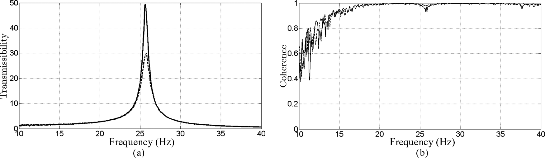
(a) Transmissibility and (b) coherence plots when the device is excited with a low level of random input displacement, that is, 0.0054 mm (rms); open-circuit (solid) and 200 Ω (dashed).

The trend of the power-harvested curve for hardening devices follows a similar trend as discussed in the previous sub-section which depends on the non-linearity and the amount of damping in the system. Figure 10 shows the maximum powers harvested by both mechanisms by the load resistance under similar excitation level, that is, Y = 0.2 mm. It can be seen that for the linear system, the optimal resistance for maximum power transfer is around 150 Ω and 90 Ω for the hardening system.

Figure 10.

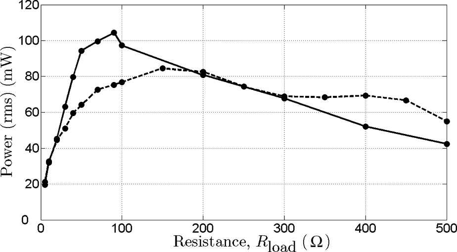
The maximum power harvested as a function of the load resistance, $R_{load}$ , for both hardening (solid) and linear (dashed) modes for the system with L = 42.70 mm, d = 1.50 mm and Y = 0.2 mm.

The condition for maximum power transfer for the linear system employing electromagnetic transduction has already been established (Stephen, 2006), while the study on the maximum power transfer of the hardening system is not yet available. However, the interpretation of this optimum power harvested by the hardening system has to be done carefully. For the linear system, the maximum power occurs at approximately the same frequency for all resistances. For a given non-linearity, the maximum power harvested by the hardening mechanism occurs at different frequency (i.e. the jump-down frequency) depending on the amount of damping (i.e. the resistance) in the system. Thus, the interpretation of the optimal resistance and frequency is not as straightforward as the linear system and the tuning maybe more complicated. In the experiment, the jump-down point can be reached easily by sweeping the frequency up. In a practical application with a tonal input frequency, it may not be easy to drive the system on the resonant branch in the region between the jump-up and jump-down points without applying the appropriate initial conditions.

Estimation of the bandwidth of the hardening mode

One significant advantage of the non-linear hardening mechanism over the linear mechanism is that the non-linear mechanism can provide a wider bandwidth over which the device can be useful (Barton et al., 2010; Mann and Sims, 2009; Ramlan et al., 2010). This is due to the capability of the mechanism to bend the FRC to the right. The maximum shift of the resonance frequency (i.e. the jump-down frequency) depends on the non-linearity and the amplitude of excitation. The amount of damping in the system also plays an important role in shifting this resonance frequency; for a given non-linearity, the smaller the damping the higher the jump-down frequency.

The estimates of the non-linearity and the damping ratio discussed in the study by Ramlan et al. (2009) allows a reliable estimate of the bandwidth to be made using the expression derived in the study by Ramlan et al. (2010) by just using the jump-up and the jump-down frequencies. Figure 11 shows a comparison between the bandwidth of the linear and the hardening mechanisms as a function of the load resistance (i.e. damping). The damping of the linear device was determined using the log decrement method. The damping contributes to half of the bandwidth of the linear device. It can be seen that the bandwidth of the hardening system is greater than the linear system even when the non-linearity is relatively small, as shown by the dashed line. It can also be seen that the bandwidth is greater when the damping in the system is small (i.e. large resistance). The bandwidth of the hardening system also depends strongly on the non-linearity. The bandwidth of the system with a stronger non-linearity is shown by the dotted line which represents the same system when the input displacement is doubled at 0.2 mm.

Figure 11.

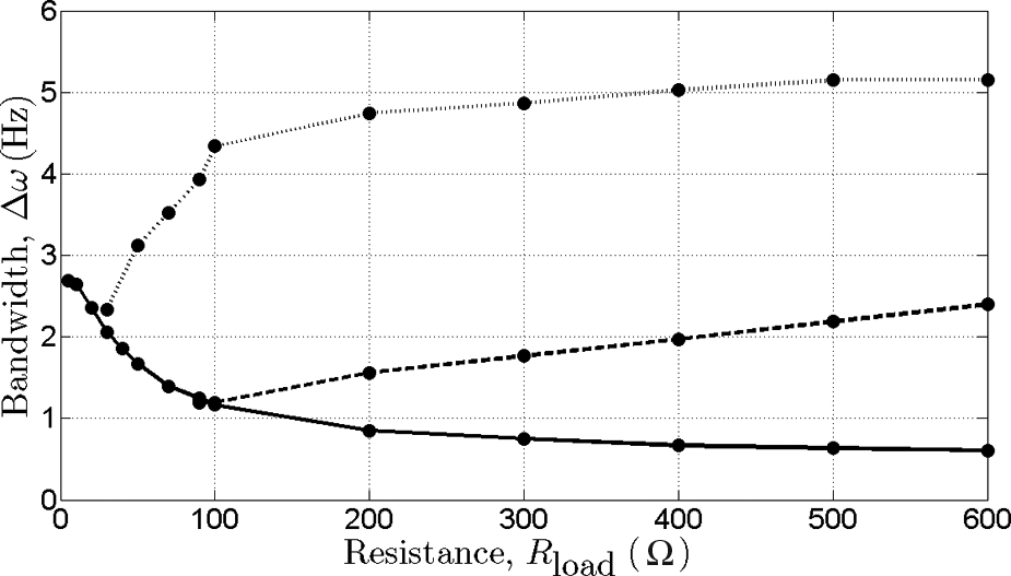
Estimate of the bandwidth of the linear and hardening modes; linear (solid), hardening (input = 0.1 mm, dashed) and hardening (input = 0.2 mm, dotted) for the system with L = 42.70 mm and d = 1.50 mm.

Thus, the device could be useful over a wide frequency range by having a large non-linearity and a small damping in the system. However, the performance of the hardening mechanism may be reduced due to the response not being on the resonant branch (upper branch) in the region between the jump-up and jump-down frequencies if inappropriate initial conditions are applied to the system.

Experimental results of the bi-stable mode

The device can be configured to behave in the bi-stable mode using a smaller gap d. The system then has two stable equilibrium positions and one unstable equilibrium position. Depending on the input level, non-linearity, damping and the initial conditions, the mass will either oscillate about one of the stable positions or across the two potential wells overcoming the central potential barrier. A comparison of the performance between the hardening and bi-stable modes of the device is not possible because the input level used in the hardening mode was not high enough to throw the mass between the two stable positions in the bi-stable mode.

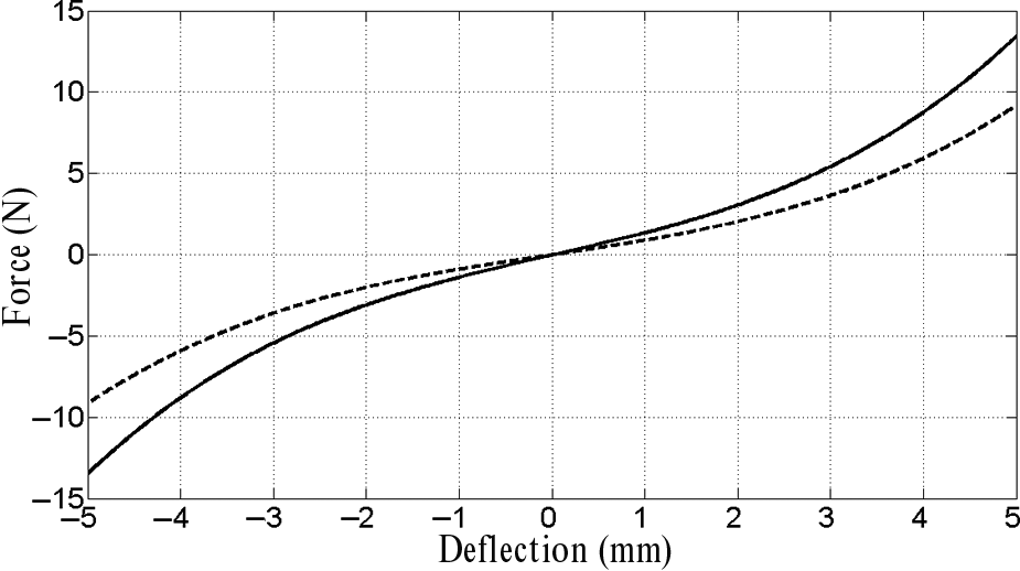
The experimental results for the bi-stable mode are presented in this section. The aim of the experiment was to investigate how the dynamics of such a system is affected by the non-linearity, input level and the damping. For the bi-stable mode, the smaller the gap $d$ results in a higher non-linearity, and the larger the non-linearity, the more difficult it is to throw the mass from one stable position to another. It is important to note that the results presented in this section may not be comparable to the results reported in the study by Cammarano et al. (2011) due to different configurations used during the experiment since this particular device is very sensitive to the input level, damping, gap and the length of the beam.

Figure 12 shows the fitted curve of the measured force–deflection when the gap was 0.6 mm. It can be seen that the system behaves completely different by having a small change in length $L$ and the gap $d$ . This figure also shows that the stiffness of the system changes from positive to negative between the two turning points of this curve.

Figure 12.

Measured force–deflection curve for device in bi-stable mode when the gap d = 0.6 mm.

Effect of input displacement, damping and the gap on the response and the power harvested

The response of the bi-stable mode comprises both periodic and chaotic responses depending on the frequency and amplitude of excitation and the damping. When the mass oscillates about one of the stable equilibriums, the response is mainly periodic. However, when the mass oscillates between the two stable equilibria, the response can be either chaotic or periodic. Figures 13 to 15 show the effect of the input level, damping and the non-linearity (i.e. the gap) on the response of the bi-stable mode device. Due to possible chaotic behaviour, the rms values of the response are measured over 20 excitation periods.

Figure 13.

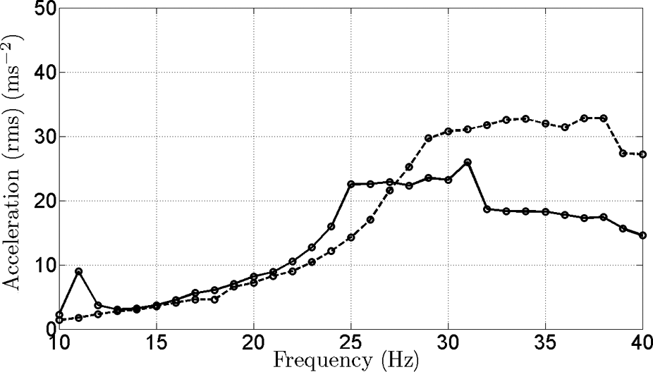
The measured response of the rms acceleration when R_load = 200 Ω using different levels of input displacement; 0.4 mm (dashed) and 0.5 mm (solid).

Figure 14.

The measured response of the rms acceleration when the gap d = 0.6 mm and 0.4 mm input displacement for different resistances; open-circuit (solid) and R_load = 200 Ω (dashed).

Figure 15.

The measured response of the rms acceleration when R_load = 200 Ω and 0.4 mm input displacement for different gaps; 0.8 mm (solid) and 0.6 mm (dashed).

Figure 13 shows the measured rms acceleration response of the bi-stable mode for different input levels, that is, 0.4 and 0.5 mm. It can be seen that the response is initially very small at low frequencies, which means that the mass oscillates in one of the potential wells only as discussed in the study by Ramlan (2009). When the frequency is increased, the amplitude of the response increases suddenly which shows that the oscillation of the mass is between the two potential wells. The frequency where the mass starts to oscillate between the two potential wells depends on the level of input, the amount of damping and the gap, that is, the non-linearity. It is shown in Figure 13 that the cross-well motion is initiated in the system with a larger input at a lower frequency than the one with a smaller input since the one with the larger input can overcome the potential barrier even at a lower frequency.

The effect of damping (i.e. resistance) on the response is shown in Figure 14. With the same input level, the one with a smaller damping jumps between the two equilibrium positions at a lower frequency than the one with a larger damping. This is because there is less resistance to motion in the system with smaller damping.

Figure 15 compares the response for the system with different gaps under the same level of input displacement. It can be seen that the larger the non-linearity, the more difficult it is for the mass to oscillate across the two potential wells (Ramlan et al., 2010). The response for the system with d = 0.8 mm starts to cross between the two potential wells at a lower frequency than the one when the gap is 0.6 mm. It can also be seen that after the jump occurs, the responses start to oscillate at an approximately constant level for a certain frequency region and then start to vibrate about one of the equilibrium position again when the frequency is further increased. This behaviour is probably due to the increase in the impedance of the mass which makes it more difficult for the mass to move at high frequencies (Gardonio and Brennan, 2004).

The dynamic response of the bi-stable device under different conditions shows that it is insensitive to a range of excitation frequencies depending upon the degree of non-linearity, damping and input level. From the energy-harvesting point of view, this is an advantage since the device can operate over a range of frequencies without having significant degradation in the performance as shown in Figure 16. It can be seen that the trend of power harvested across the load resistor follows similar trends as the FRCs shown in Figures 13 to 15. In this mode, the average power is almost flat for a range of excitation frequency. The maximum power transfer theory is less feasible here since the device with this mode contributes more towards the bandwidth rather the maximum power as shown in Figure 16. This figure shows that the bi-stable mode may provide a better bandwidth but a relatively small amount of power.

Figure 16.

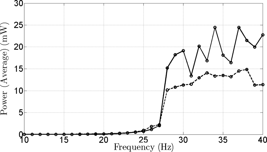
The measured average power harvested across load resistance R_load = 200 Ω using different levels of input displacement; 0.4 mm (dashed) and 0.5 mm (solid).

Conclusion

This article has presented experimental results for a dual-mode non-linear energy harvesting device. The device is capable of operating in hardening and bi-stable modes. The change from one mode to another is made possible by altering the negative stiffness produced by the magnets. This is done by adjusting the separation gap between the magnets and the iron core.

The dynamic response of the device in the hardening mode showed that the performance of the device depends on the linear and non-linear stiffness, the excitation level and the damping. It was also shown that the bandwidth of the device can be wider than the equivalent linear device.

The maximum power transfer concept for both hardening and linear devices was also investigated. It was found that the maximum power transfer to the load for a hardening mode occurred at different frequency depending upon the non-linearity and the damping. Thus, finding a suitable condition for maximum power transfer to the load is not as easy as the linear device in which the maximum power transfer occurs at almost the same frequency.

The effect of the non-linearity (i.e. gap), damping and the input level on the dynamics of the system was also investigated for the bi-stable mode. It was found that the response of the device was insensitive to a range of excitation frequencies, which shows the benefits of this device in increasing the bandwidth of operation.

Footnotes

Funding

This study was supported by the Government of Malaysia through the Ministry of Higher Education Malaysia and the Universiti Teknikal Malaysia Melaka (UTeM) under the Bumiputera Academic Training Scheme (SLAB) scholarship award.

References

Andò

Baglio

Trigona

. (2010) Nonlinear mechanism in MEMS devices for energy harvesting applications. Journal of Micromechanics and Microengineering 20(12): 125020-1–125020-12.

Arrieta

Hagedorn

Erturk

. (2010) A piezoelectric bistable plate for nonlinear broadband energy harvesting. Applied Physics Letters 97(10): 104102-1–104102-3.

Barton

DAW

Burrow

Clare

(2010) Energy harvesting from vibrations with a nonlinear oscillator. Journal of Vibration and Acoustics 132: 021009-1–021009-7.

Bowers

Arnold

(2009) Spherical, rolling magnet generators for passive energy harvesting from human motion. Journal of Micromechanics and Microengineering 19: 094008.

Brennan

Kovacic

Carella

. (2008) On the jump-up and jump-down frequencies of the Duffing oscillator. Journal of Sound and Vibration 318(4–5): 1250–1261.

Burrow

Clare

(2007) A resonant generator with nonlinear compliance for energy harvesting in high vibrational environments. In: IEEE international conference on electric machines and drives, Antalya, Turkey, 3–5 May 2007.

Cammarano

Burrow

Barton

DAW

(2011) Modelling and experimental characterization of an energy harvester with bi-stable compliance characteristics. Proceedings of IMechE, Part I: Journal of Systems and Control Engineering 225: 475–484.

Cammarano

Burrow

Barton

DAW

. (2010) Tuning a resonant energy harvester using a generalized electrical load. Smart Materials and Structures 19(5): 055003.

Erturk

Inman

(2011) Broadband piezoelectric power generation on high-energy orbits of the bistable Duffing oscillator with electromechanical coupling. Journal of Sound and Vibration 330(10): 2339–2353.

10.

Gardonio

Brennan

(2004) Advanced applications in acoustics, noise and vibration. In: Fahy

Walker

(eds) Mobility and Impedance Methods. Ch. 9. London and New York, NY: Spon Press. Page: 389–447

11.

Kovacic

Brennan

(2011) The Duffing Equation: Nonlinear Oscillators and their Behaviour. Chichester: John Wiley and Sons, Ltd.

12.

Külah

Najafi

(2008) Energy scavenging from low-frequency vibrations by using frequency up-conversion for wireless sensor applications. IEEE Sensors Journal 8(3): 261–268.

13.

Litak

Friswell

Adhikari

(2010) Magnetopiezoelastic energy harvesting driven by random excitations. Applied Physics Letters 96(21): 214103.

14.

McInnes

Gorman

Cartmell

(2008) Enhanced vibrational energy harvesting using nonlinear stochastic resonance. Journal of Sound and Vibration 318(4–5): 655–662.

15.

Mann

Owens

(2010) Investigations of a nonlinear energy harvester with a bistable potential well. Journal of Sound and Vibration 329(9): 1215–1226.

16.

Mann

Sims

(2009) Energy harvesting from the nonlinear oscillations of magnetic levitation. Journal of Sound and Vibration 319(1–2): 515–530.

17.

Quinn

Triplett

Bergman

. (2011) Comparing linear and essentially nonlinear vibration-based energy harvesting. Journal of Vibration and Acoustics-Transactions of the ASME 133(1): 011001-1–011001-8.

18.

Ramlan

(2009) Effects of non-linear stiffness on performance of an energy harvesting device. PhD Thesis, University of Southampton, UK.

19.

Ramlan

Brennan

Mace

(2008) Nonlinear bistable mechanism for energy harvesting devices. In: 7th European conference on structural dynamics (Eurodyn 2008), Southampton, UK, 7–9 July 2008.

20.

Ramlan

Brennan

Mace

. (2009) On the estimation of linear viscous damping in the Duffing oscillator. In: Proceedings of the 16th international congress on sound and vibration, Krakow, Poland, 5–9 July 2009.

21.

Ramlan

Brennan

Mace

. (2010) Potential benefits of a non-linear stiffness in an energy harvesting device. Nonlinear Dynamics 59(4): 545–558.

22.

Stanton

McGehee

Mann

(2010) Nonlinear dynamics for broadband energy harvesting: investigation of a bistable piezoelectric inertial generator. Physica D: Nonlinear Phenomena 239(10): 640–653.

23.

Stephen

(2006) On the maximum power transfer theorem within electromechanical systems. Proceedings of the Institution of Mechanical Engineers, Part C: Journal of Mechanical Engineering Science 220: 1261–1267.

24.

Tang

Yang

Soh

(2010) Toward broadband vibration-based energy harvesting. Journal of Intelligent Material Systems and Structures 21(18): 1867–1897.

25.

Williams

Yates

(1996) Analysis of a micro-generator for microsystems. Sensors and Actuators A: Physical 52: 8–11.

26.

Zhu

Tudor

Beeby

(2010) Strategies for increasing the operating frequency range of vibration energy harvesters: a review. Measurement Science and Technology 21(2): 1–29.