Physical modeling and design method of the hysteretic behavior of magnetorheological dampers

Abstract

This study aims to get a deep insight of the inherent hysteresis behavior of magnetorheological fluid dampers and to develop the method of designing such hysteresis. Taking into account the compressibility of magnetorheological fluid, a physical model of magnetorheological dampers is developed by establishing the flow rate equations for two chambers. The model is validated by a set of the experimental data from a literature. As a special case of the proposed physical model, a lumped parameter physical model which can explain the hysteresis in a more straightforward way is derived and validated too. The fact that the viscous force can be ignored compared to the Coulomb force reduces the lumped parameter physical model to its simplest form, that is, a friction element representing the Coulomb force is connected in series with a spring element representing the compressibility of fluid. It is this simple two-element physical model that captures the essence of the hysteresis behavior, on the basis of which, the mechanism of the hysteresis generation is explored in great detail, and the formula is also derived for calculating the hysteresis width. Finally, the design method of the hysteresis behavior is illustrated by a specific example.

Keywords

Magnetorheological damper compressibility hysteresis physical modeling design method

Introduction

Possessing advantages of large damping force, high reliable operation, and low power requirements, magnetorheological (MR) fluid dampers have become one of the most promising semi-active control devices for civil structures (Ali and Ramaswamy, 2009; Dyke et al., 1999), automobiles (Giorgetti et al., 2010; Gordaninejad and Kelso, 2000; Sassi et al., 2005), and aircrafts (Batterbee et al., 2007a, 2007b; Lee et al., 2009).

A typical configuration of MR dampers is shown in Figure 1. When excited by a certain constant input electric current, the steady damping forces of an MR damper operated at constant piston velocities monotonously increases with the piston velocity, as shown in Figure 2. This one-to-one relationship between the damping force and piston velocity is a fundamental damping capacity index of a damper and can be predicted by the quasi-static models in great accuracy. Actually, the quasi-static models have been the main tool in designing dampers, and the Bingham model is the one most widely used due to its simplicity.

Figure 1.

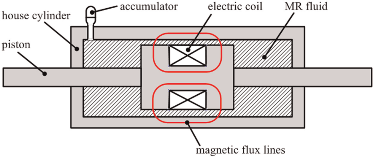
Typical configuration of an MR damper.

Figure 2.

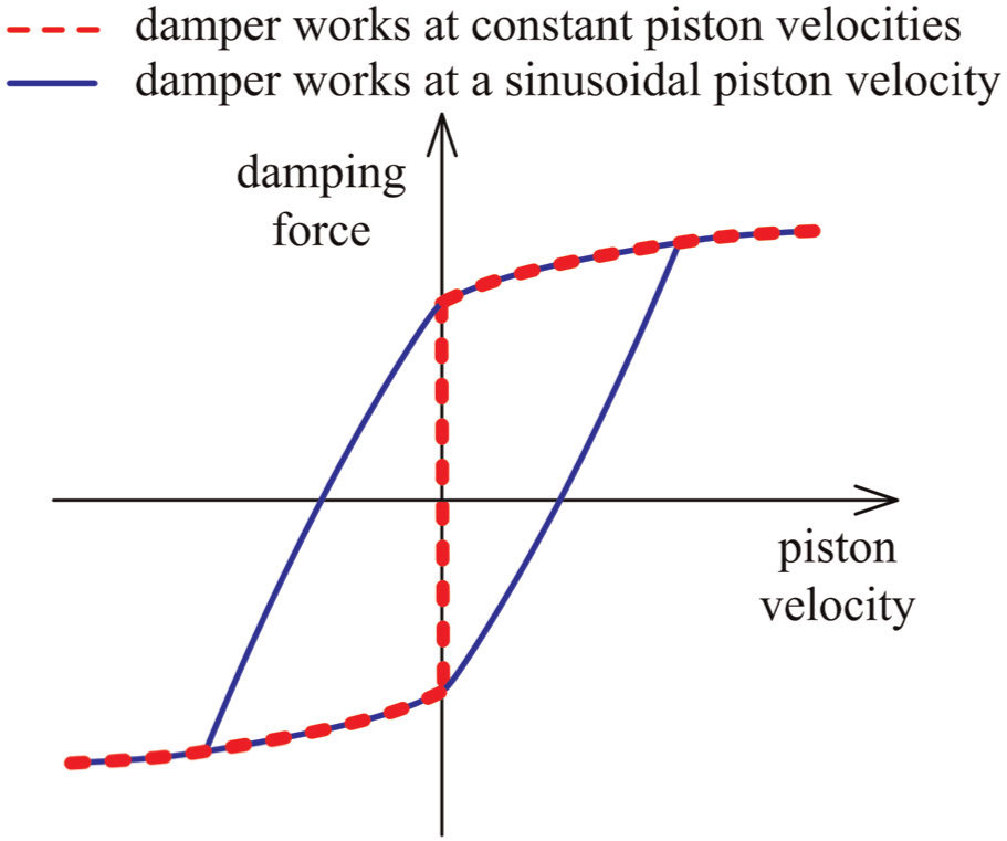
Monotonously varied damping force when the piston is operated at constant velocities versus hysteretic damping force at a sinusoidal velocity. The input electric current is fixed.

Different from the above one-to-one force–velocity relationship, the hysteretic behavior as shown in Figure 2 is observed when a damper is operated at a sinusoidal piston velocity. Many dynamic models have been developed to study this hysteresis behavior and show satisfying predicting accuracies with many of them having been used in practical MR-based vibration control engineering. These models, comprehensively summarized and compared by Şahin et al. (2010) and Wang and Liao (2011), can be classified into two main categories as parametric and nonparametric ones. The former is more favored because the model parameters have physical meanings, and it includes the hysteretic Bingham plastic model (Spencer et al., 1997), the hysteretic Biviscous model (Wereley et al., 1998), the nonlinear viscoelastic plastic model (Kamath and Wereley, 1997), the Bouc–Wen model (Spencer et al., 1997), and the Dahl model (Zhou et al., 2006). The nonparametric models usually completely disregard the physical meanings of the model parameters, and typical ones are the polynomial model (Choi et al., 2001; Gavin et al., 1996), the generalized sigmoid function model (Ma et al., 2002), neural networks (Chang and Roschke, 1998; Chang and Zhou, 2002; Du et al., 2006; Wang and Liao, 2004), and neuro-fuzzy (Schurter and Roschke, 2000; Wilson and Abdullah, 2005).

However, the existing parametric models need experimental data to identify the model parameters, so the prediction abilities not only rely on the dynamic model themselves but also rely on the identification methods (Wang and Liao, 2011). Moreover, there exist artificialities when constructing these models and interpreting the physical meanings of the model parameters, so they are essentially phenomenological models. For example, compared with the Bouc–Wen model (Spencer et al., 1997), the introduction of accumulator stiffness (k₁) and the dashpot (c₁) in the modified Bouc–Wen model (Spencer et al., 1997), as shown in Figure 3, is an attempt to produce the roll-off that was observed in the experimental data at low velocities.

Figure 3.

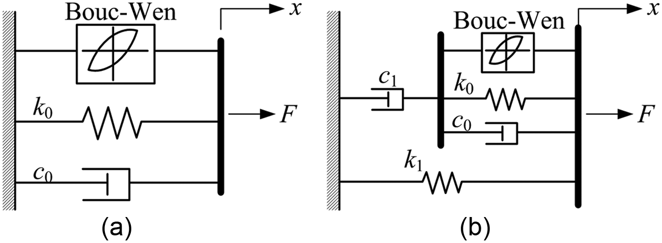
Comparison of (a) the Bouc–Wen model with (b) the voltage-dependent modified Bouc–Wen model.

In addition, these models coexist with certain specific MR dampers, which have been already fabricated and tested with sufficient experimental data acquired. However, it is often more desirable to know the factors affecting the dynamic behavior of an MR damper before it is fabricated, that is, to understand the physical mechanism behind the hysteresis behavior.

Only by a physical model can such essential understanding be achieved, and several efforts have been made to develop the physical models of MR dampers. Notably, phenomenological models close to physical models were developed by Peel et al. (1996), Sims et al. (1999), and Hong et al. (2005), but some key model parameters, such as the stiffness, are still need to be identified using experimental data. Combining the Herschel–Bulkley quasi-static model with the mass flow rate continuity, Wang and Faramarz (2007) derived a physical model of MR dampers, and the hysteresis behavior was found to be contributed by the compressibility of MR fluid. However, the effect of air content was oversimplified by the assumption that the fluid bulk was a pressure-independent constant, while Akkaya’s (2006) study suggested that fluid bulk modulus should be considered as a variable to achieve a more realistic hydraulic model. Recently, by considering high-speed losses, fluid chamber compressibility, cavitations, elastic deformation of cylinder, fluid inertia, and so on, a lumped parameter physical model was developed by Goldasz and Sapinski (2013) to study MR shock absorbers with different piston configurations. It is interesting that the fluid inertia was found to be responsible for the force oscillations occurring when the piston reverses its direction. By applying the combination of Laplace and Weber transforms to the Navier–Stokes equations to obtain the analytical solutions of the velocity and using Duhamel’s superposition integral to include the time-variant piston velocity, a transient physical model of great predicting accuracy for dynamic performances of MR dampers was developed by Bhatnagar (2013), and the hysteresis-like variation of force versus velocity was concluded to be a consequence of the variation of the piston velocity.

In this article, a physical hysteretic model of MR dampers and its equivalent lumped versions will be proposed by basically incorporating a quasi-static model with the consideration of the compressibility of MR fluid, and the models will be validated by the experimental data from a literature. Analysis based on these models will be performed, especially on the lumped ones, to essentially understand the hysteresis behavior of MR dampers. Compared to the available studies, the efforts toward the following contributions are made:

As an extension of the works by Wang and Faramarz (2007) and by Goldasz and Sapinski (2013), a more comprehensive physical hysteretic model is developed in which effect of the air content can be included.

More importantly, the underlying physical process (or the mechanism) of the hysteresis generation of MR dampers is explored in detail.

The formula for calculating the hysteresis is derived, which makes it possible to design the hysteresis, and such design method is also demonstrated.

Quasi-static models: modeling and designing damping force of MR dampers operated at constant piston velocities

Before modeling the hysteresis behavior, it is necessary to introduce the quasi-static models of MR dampers, which also explain the working principles of an MR damper. The governing equation for the MR fluid flowing through the working gap can be derived by the Navier–Stokes equation as

\frac{d τ (y)}{dy} = - p'

(1)

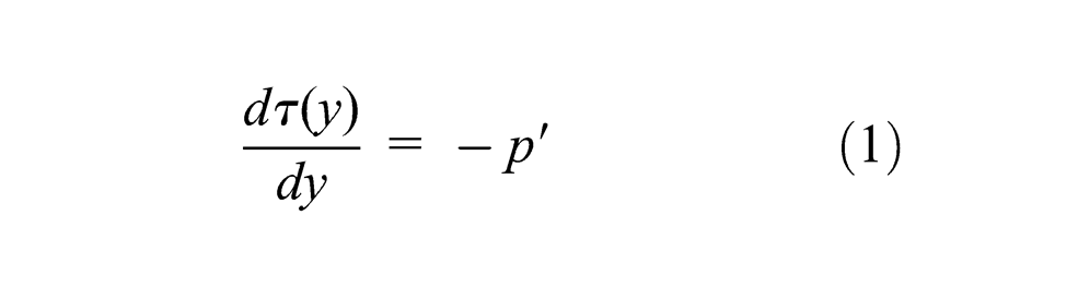
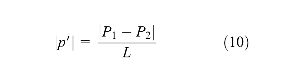
where τ is the shear stress, y is the coordinate measured from the center of the annular gap to the inside wall of the house cylinder, and p′ is the pressure gradient, and p′ = ΔP/L, where L is the effective length of the piston and ΔP is the pressure drop from the flow inlet to the flow outlet, and ΔP = F/A, where F is the damper force and A is the effective area of the piston head.

The shear stress (τ) in equation (1) is related to the piston velocity by the constitutive model (f) of MR fluid as

τ = f (γ) = f (\frac{du}{dy})

(2)

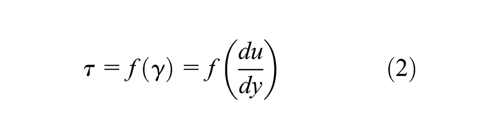
where u and γ are the flow velocity and shear strain, respectively, of MR fluid in the working gap.

Substituting equation (2) into equation (1), a quasi-static model of MR dampers is established as a second-order ordinary differential equation (ODE) for the flow velocity or a system of ODEs when piecewise material models are adopted. Solving these ODEs, the integration of the flow velocity over the gap gives the damping force in terms of the piston velocity. Based on different material models, a number of MR damper models have been developed, including the Bingham model (Phillips, 1969; Yang, 2001), the Herschel–Bulkley model (Lee et al., 2002; Wang and Faramarz, 1999; Wereley, 2008), the Biviscous model (Wereley et al., 2004), and the modified Herschel–Bulkley model (Hong et al., 2008).

With a sufficient engineering accuracy, the fixed parallel plate flow is frequently used to model the axisymmetric flow of MR fluid in MR dampers, and a general solution was derived by Guan and Guo (2011) for such flow problem. As an application of this general solution, a unified quasi-static damper model was proposed with the corresponding constitutive model shown in Figure 4(a). Both the nonlinear yielding process of MR fluid and the shear-thinning effect (Figure 4(b)) are included in this model, and the flow rate (Q) is related to the pressure gradient (p′) by

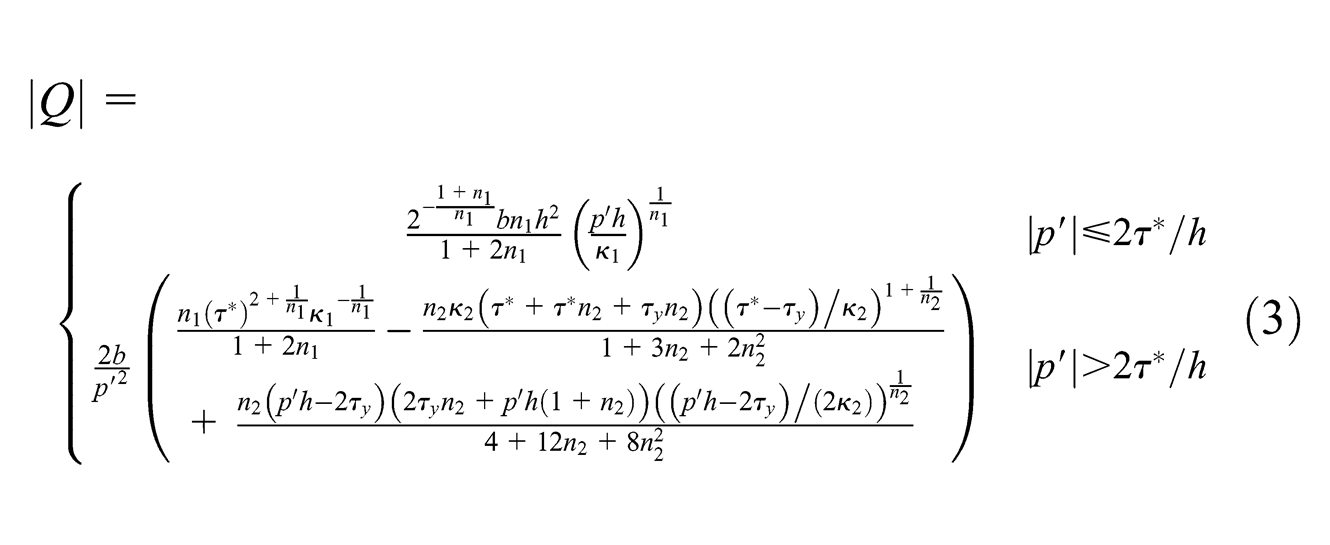
| Q | = {\begin{matrix} \frac{2^{- \frac{1 + n_{1}}{n_{1}}} b n_{1} h^{2}}{1 + 2 n_{1}} {(\frac{p' h}{κ_{1}})}^{\frac{1}{n_{1}}} & | p' | \leq 2 τ^{*} / h \\ \frac{2 b}{{p'}^{2}} (\begin{matrix} \frac{n_{1} {(τ^{*})}^{2 + \frac{1}{n_{1}}} {κ_{1}}^{- \frac{1}{n_{1}}}}{1 + 2 n_{1}} - \frac{n_{2} κ_{2} (τ^{*} + τ^{*} n_{2} + τ_{y} n_{2}) {((τ^{*} - τ_{y}) / κ_{2})}^{1 + \frac{1}{n_{2}}}}{1 + 3 n_{2} + 2 n_{2}^{2}} \\ + \frac{n_{2} (p' h - 2 τ_{y}) (2 τ_{y} n_{2} + p' h (1 + n_{2})) {((p' h - 2 τ_{y}) / (2 κ_{2}))}^{\frac{1}{n_{2}}}}{4 + 12 n_{2} + 8 n_{2}^{2}} \end{matrix}) & | p' | > 2 τ^{*} / h \end{matrix}

(3)

where, as shown in Figure 4(a) and (b), all the parameters but the pre-yield flow index, n₁, have the same physical meanings as those in the modified Herschel–Bulkley model, that is, n₂ is the post-yield flow index and κ₁ and κ₂ are consistencies which are analogous to fluid viscosities and specialize to the pre-yield and post-yield viscosities in the Biviscous model when n₁ = n₂ = 1; τ^* and τ_y are the dynamic and static shear yield stresses of MR fluid, h is the working gap of MR dampers, and b is the average circumstance of the gap.

Figure 4.

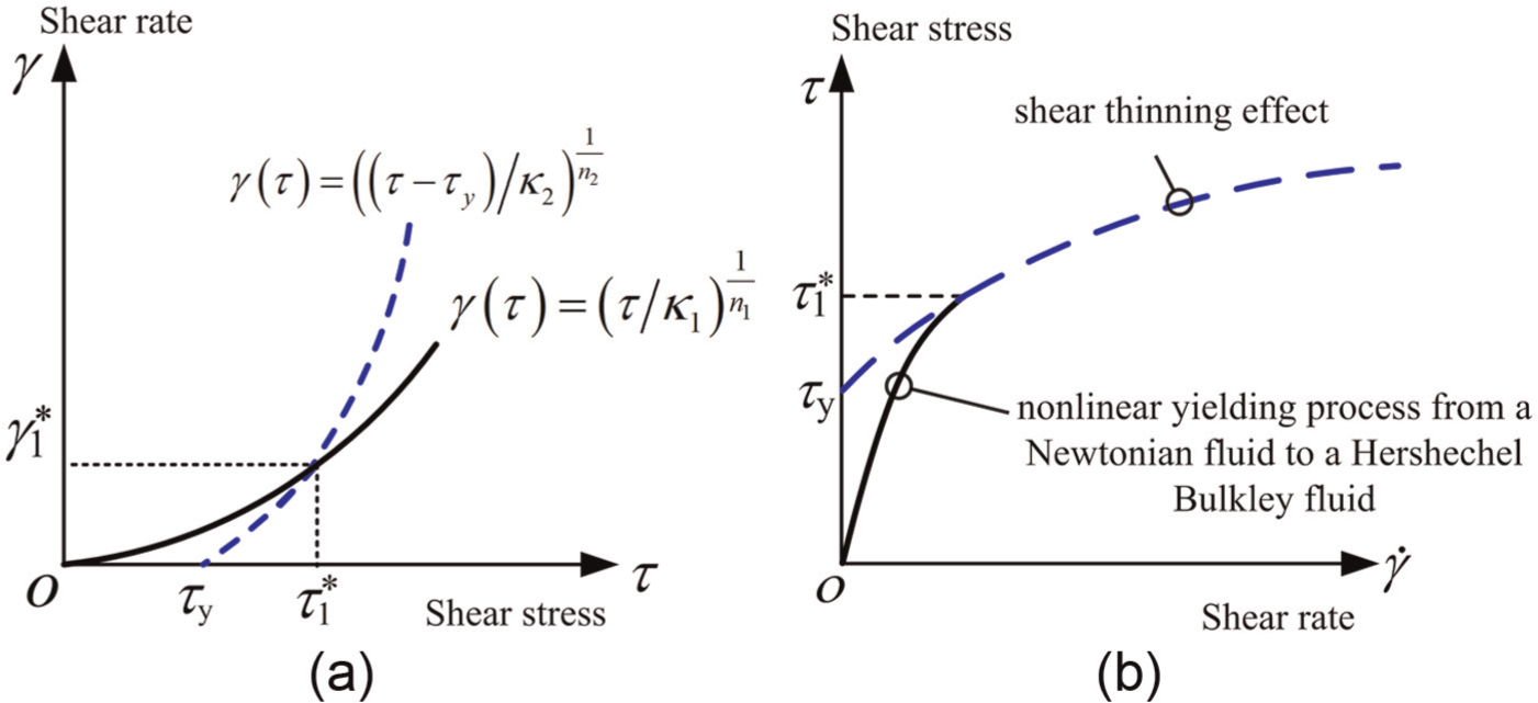
(a) A general quasi-static constitutive model of MR fluid with both (b) the pre- and post-yield material nonlinearities included (Guan and Guo, 2011).

A physical hysteretic model of MR dampers

Flow rate equation based on the compressibility of fluid

Generally, the damping force of a fluid damper is closely related to the volume rate of the working fluid in the gap. However, the compressibility of fluid generally deteriorates a damper’s performance, and the entrapped air bubbles are usually the main factor greatly reducing the bulk modulus of a fluid, thus making the compressibility be no longer ignored. For this reason, the entrapped air is often considered as “pollution” for engineering hydraulic oils.

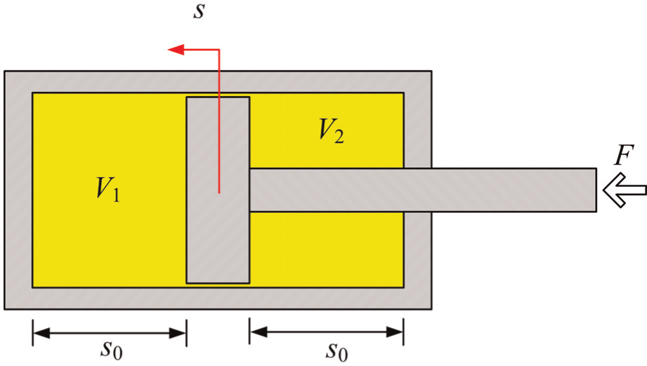
Unfortunately, determination of the time-dependent air content in an MR damper is challenging and greatly complicated by the transportation of air bubbles from one chamber to the other, so several assumptions are made for both the gap and the chambers to simplify the derivation of the volumetric rate of MR fluid. The compressibility of the mixture in the gap is ignored due to its small volume. Normally, the variation of the air volume fraction in each chamber is mainly dominated by the changes of the chamber pressure and chamber volume (with the effect of temperature beyond the scope of this study), so the transportation of air bubbles through the gap is also neglected. Based on these assumptions, air bubbles are entrapped in each chamber as if they were “locked inside,” that is, they cannot escape from one chamber to the other, with the pure (air-free) MR fluid is exchanged by two chambers, as shown in Figure 5. The whole steel part of an MR damper is considered to be a rigid body.

Figure 5.

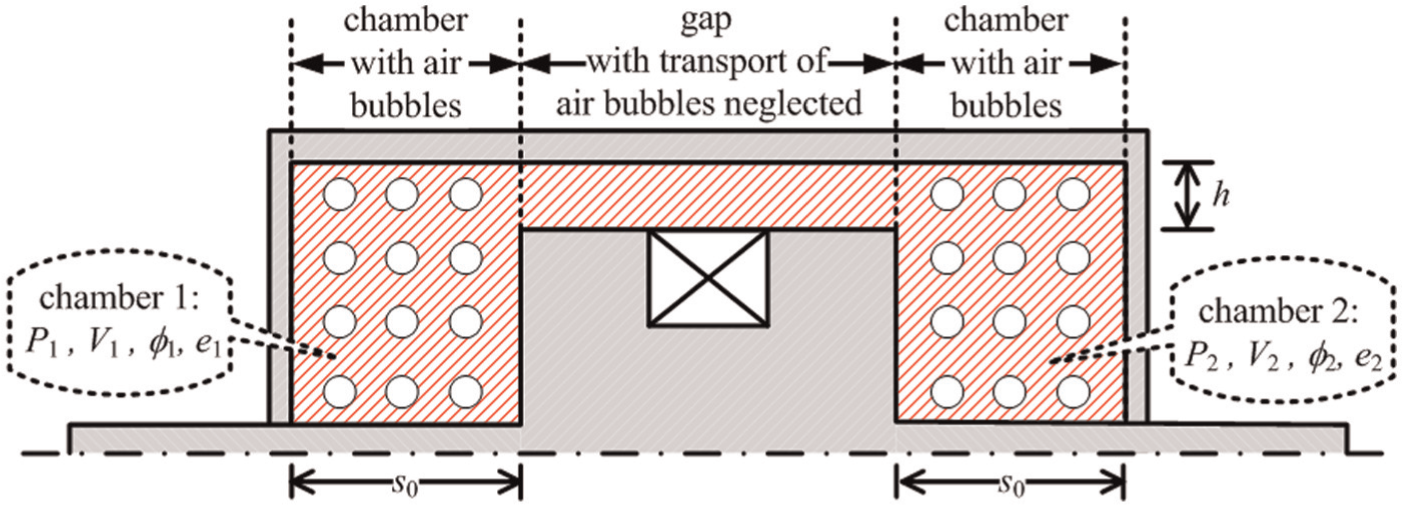
Assumptions made on the chambers and the gap to simplify the physical modeling of MR dampers.

Beside the chamber volume change because of the movement of the piston, the amount of the MR fluid flowing into (or out of) the chamber is also governed, at the same time, by the compression (or expansion) of the mixture. These two simultaneously occurring volume changes can be resolved into an isobaric process with only the chamber volume changed and an isochoric process with only the chamber pressure changed, as shown in Figure 6.

Figure 6.

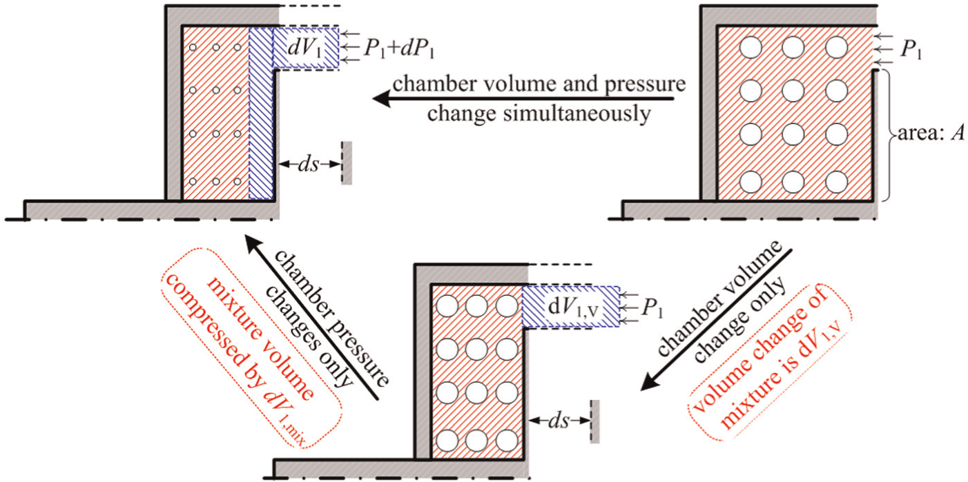
Simultaneous changing of chamber volume and pressure decomposed to an isobaric process and an isochoric process.

It is evident that in the isobaric process, the volume change of the fluid in the chamber equals to that of chamber itself. In the isochoric process, the mixture volume decreases (or increases) with the increasing (or decreasing) chamber pressure, leading to a compensating fluid flowing into (out of) the chamber, as shown in Figure 6. In other words, a positive volume change for the mixture (dV_1,mix > 0), caused by a negative chamber pressure change (dP₁ < 0), results in a negative volume change for the MR fluid in the chamber. To be clear, the volume change of MR fluid in chamber 1 is listed in Table 1 as a consequence of a positive volume change of the chamber or the mixture.

Table 1.

The volume change of MR fluid in chamber 1 arising from the positive volume change of the chamber or the mixture.

Volume changes	dV ₁ > 0	dV _1,mix > 0
Isochoric/isobaric process	Chamber volume change in the isobaric process	Mixture volume change in the isochoric process
Caused by	Piston movement (if moving rightward as shown in Figure 6)	Chamber pressure decreases (if dP₁ < 0 as shown in Figure 6)
Resulting in inward or outward flowing fluid	Inward	Outward
Volume change of MR fluid (dV_1,f) in chamber 1	Increase	Decrease

MR: magnetorheological.

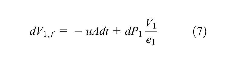
Then, the total volume change of the MR fluid in chamber 1 due to the combination of the two processes, during an infinitesimal time variation, dt, is

d V_{1, f} = d V_{1} - d V_{1, mix}

(4)

where dV_1,f, dV₁, and dV_1,mix are the volume changes of the MR fluid, the chamber, and the mixture, respectively.

Taking leftward (in Figures 5 and 6) as the positive for the piston velocity, then the chamber volume change is

d V_{1} = - uAdt

(5)

where u is the piston velocity and A is the effective area of piston head.

According to the definition of bulk modulus, the amount of the mixture volume compressed or expanded is

d V_{1, mix} = - d P_{1} \frac{V_{1}}{e_{1}}

(6)

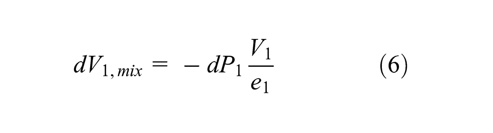
where P₁ is the pressure in chamber 1, V₁ is the volume of chamber 1, and e₁ is the bulk modulus of the mixture in chamber 1.

Consequently, the fluid volume change in chamber 1 takes the form

d V_{1, f} = - uAdt + d P_{1} \frac{V_{1}}{e_{1}}

(7)

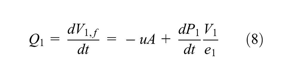
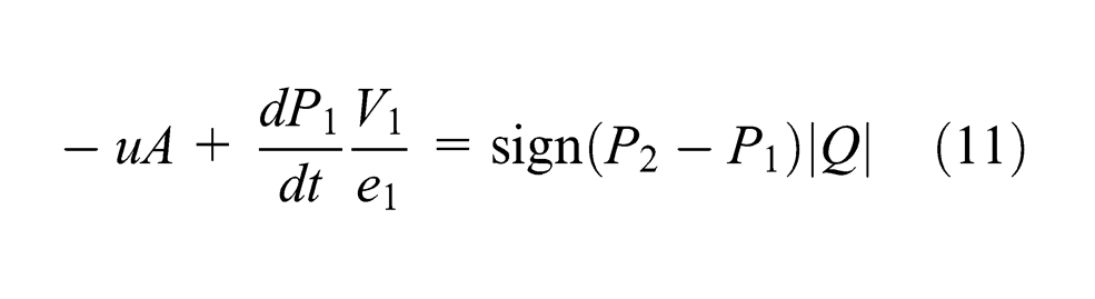
Accordingly, the flow rate for chamber 1 is

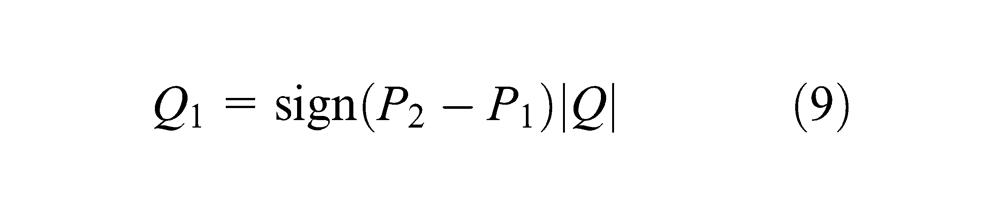
Q_{1} = \frac{d V_{1, f}}{dt} = - uA + \frac{d P_{1}}{dt} \frac{V_{1}}{e_{1}}

(8)

Considering that the sign of the flow rate for chamber 1 is determined by that of the pressure difference, P₂−P₁, that is

Q_{1} = sign (P_{2} - P_{1}) | Q |

(9)

where $| Q |$ is given by equation (3) in which the pressure gradient is expressed as

| p' | = \frac{| P_{1} - P_{2} |}{L}

(10)

It follows that

- uA + \frac{d P_{1}}{dt} \frac{V_{1}}{e_{1}} = sign (P_{2} - P_{1}) | Q |

(11)

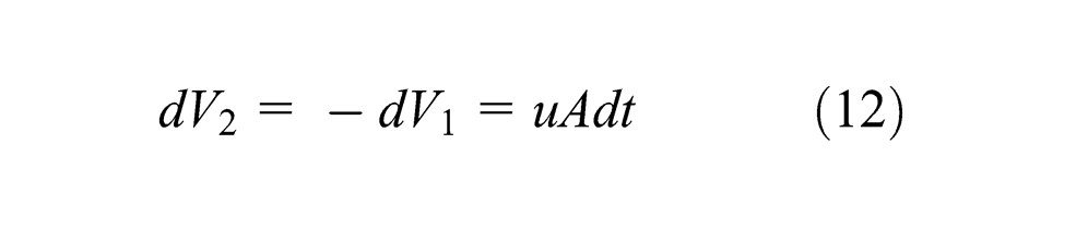
The flow rate equation can be derived similarly for chamber 2. Noting that the movement of the piston leads to an increase in the MR fluid volume in one chamber but a decrease in the other, the chamber volume change for chamber 2 can be expressed as

d V_{2} = - d V_{1} = uAdt

(12)

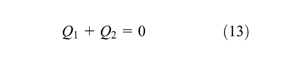
Moreover, the incompressibility assumption of the fluid in the gap yields the following flow rate continuity equation in the gap

Q_{1} + Q_{2} = 0

(13)

Then, the flow rate for chamber 2 becomes

uA + \frac{d P_{2}}{dt} \frac{V_{2}}{e_{2}} = sign (P_{1} - P_{2}) | Q |

(14)

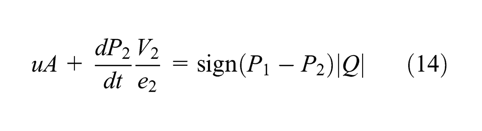
Finally, equations (3), (11), and (14) together constitute the physical model of MR dampers.

Compressibility of air–fluid mixture in the chamber

The bulk modulus of a fluid–air mixture can be estimated by (Akers et al., 2006)

e_{mix} = {(\frac{1}{e_{f}} + \frac{ϕ_{air}}{e_{air}})}^{- 1}

(15)

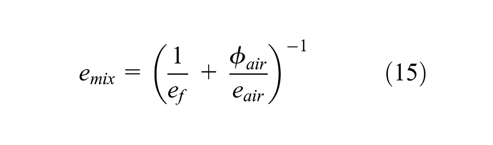
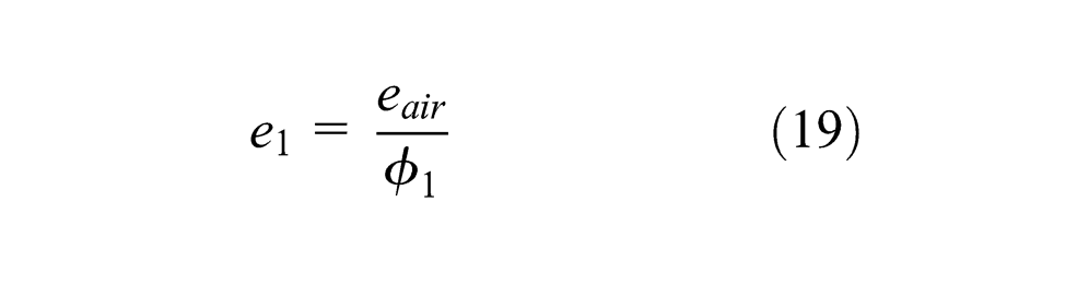
Here, for an MR damper, e_f is the modulus of MR fluid and is believed to be close to that of a standard hydraulic oil, 1.7 GPa (Batterbee et al., 2007b). φ_air is the volume content of air and e_air is the bulk modulus of air and can be computed as (Akers et al., 2006)

e_{air} = P_{air} r

where P_air is the absolute pressure and r is the polytropic exponent.

The following assumptions are made to derive the dependence of the air content on the chamber pressure

1. In both chambers, all bubbles always have the same size and they are undissolved and evenly dispersed. All the air bubbles in each chamber share the same pressure with the fluid.

For example, the gauge pressure and the volume of an arbitrary individual air bubble i in chamber 1 at time t are p_i(t) and v_i(t), equal to P₁(t) and v(t), respectively.

2. The pressures and volumes of air bubbles are governed by the polytropic law for the compression (or expansion) of gas, and for chamber 1, this is expressed as

\frac{v (t)}{v (0)} = {(\frac{P_{1} (0) + P_{atm}}{P_{1} (t) + P_{atm}})}^{1 / r}

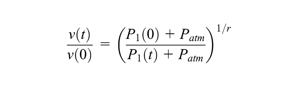
where P_atm is the atmospheric pressure, r is the polytropic exponent, v(0) is the initial volume of the air bubbles, and P₁(0) are the initial pressure of chamber 1.

Based on these assumptions, the volume of air in chamber 1, V_a₁(t), satisfies

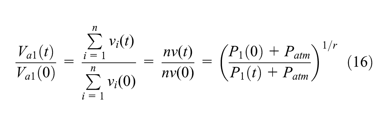
\frac{V_{a 1} (t)}{V_{a 1} (0)} = \frac{\sum_{i = 1}^{n} v_{i} (t)}{\sum_{i = 1}^{n} v_{i} (0)} = \frac{nv (t)}{nv (0)} = {(\frac{P_{1} (0) + P_{atm}}{P_{1} (t) + P_{atm}})}^{1 / r}

(16)

And it leads to

V_{a 1} (t) = {(\frac{P_{1} (0) + P_{atm}}{P_{1} (t) + P_{atm}})}^{1 / r} V_{a 1} (0)

(17)

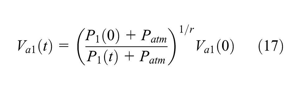
where V_a₁(0) is the initial volume of the air in chamber 1 and n is the number of air bubbles.

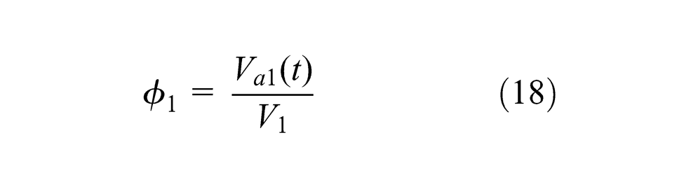
Then, the volume content of air in chamber 1 can be obtained as

ϕ_{1} = \frac{V_{a 1} (t)}{V_{1}}

(18)

However, for simplicity, the fluid in the chamber is also assumed to be incompressible, and the mixture bulk modulus is then reduced to

e_{1} = \frac{e_{air}}{ϕ_{1}}

(19)

Making use of V₁ = (s₀−s)A, the bulk modulus of the mixture in chamber 1 is finally written as

e_{1} = \frac{(P_{1} (t) + P_{atm}) r}{V_{a 1} (t)} (s_{0} - s) A

(20)

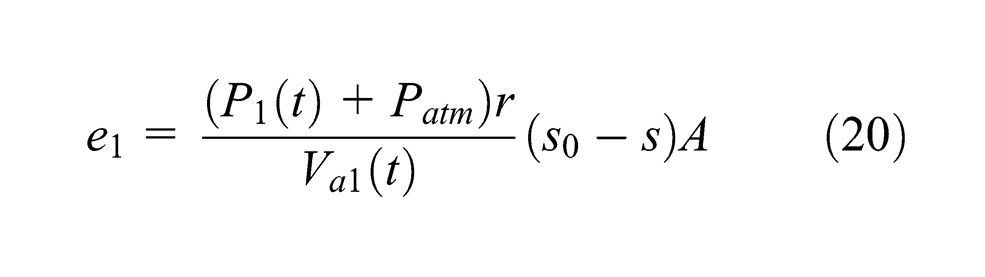
where s₀ is the stroke of a damper and s is the displacement of the piston.

Similarly, the bulk modulus of the mixture in chamber 2 is

e_{2} = \frac{(P_{2} (t) + P_{atm}) r}{V_{a 2} (t)} (s_{0} + s) A

(21)

Up to this point, the physical model of MR dampers, consisting of equations (3), (11), (14), (20), and (21), has been finally established and is ready to simulate the hysteresis behavior of MR dampers.

Validation of the proposed physical model

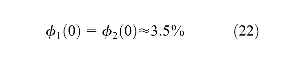
Due to the inevitable entrapped air in a fluid, especially for MR fluid which has a relatively large viscosity, serious force lag was observed in Yang’s (2001) study, and a pre-pressure of 1300 lbf/in² was applied to eliminate the force lag by pumping excessive MR fluid into the damper. The experimental study by Batterbee et al. (2007b) suggested that the modulus of the mixture of MR fluid and air is about 0.3 GPa for an MR damper working without force lag problem, much smaller than that of MR fluid, 1.7 GPa. Based on this information, the initial air content of the damper in Yang’s (2001) study, though not tested by Yang, can be estimated by equation (15) as

ϕ_{1} (0) = ϕ_{2} (0) \approx 3.5 %

(22)

Having this parameter determined, the hysteresis behavior of the damper in Yang’s (2001) study can be predicted by the proposed model and then validated by comparing the model results with his experimental data. The structure parameters of the damper as well as the fluid properties in terms of the Herschel–Bulkley model are listed in Table 2.

Table 2.

The structure of the damper and the MR fluid properties in Yang’s (2001) study.

Damper structure				Herschel–Bulkley model
Stroke (s₀)	Effective length of piston (L)	Gap (h)	Effective area of piston (A)	Post-yield flow index (n₂)	Consistency parameter (κ₂)
8 cm	84.428 cm	2.057 mm	261 cm²	1.6	33 Pa s

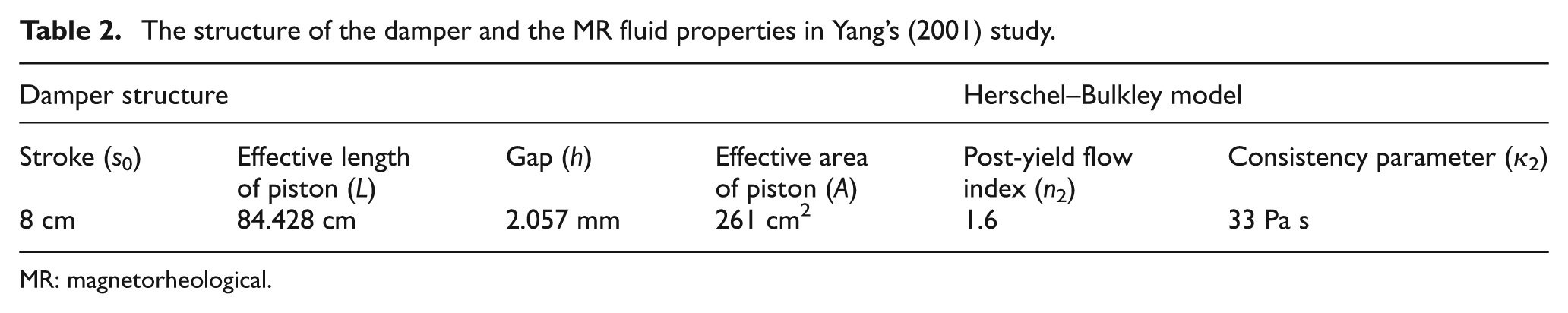
MR: magnetorheological.

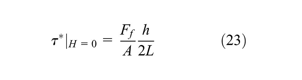
Under the sinusoidal displacement excitations listed in Table 3, the damping forces with the input currents of 0, 0.25, 0.5, 1, and 2 A are simulated. For the quasi-static model, equation (3) with a very large pre-yield viscosity, that is, κ₁ = 10⁵κ₂, instead of the Herschel–Bulkley, is used in simulation, which is expected to have a better convergence performance. The pre-yield flow index is chosen to be 1 for simplicity. It should be noted that the friction force of MR dampers, F_f, which was 3.9 kN in Yang’s (2001) experiment, acts as the shear yield stress of MR fluid, τ^*, in the absence of magnetic field (H), and the conversion relationship can be obtained by the Bingham model as (Yang, 2001)

{τ^{*} |}_{H = 0} = \frac{F_{f}}{A} \frac{h}{2 L}

(23)

Table 3.

Tests of damping force under sinusoidal displacement excitations (Yang, 2001).

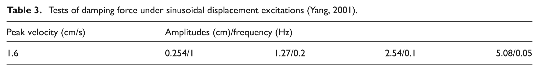
Peak velocity (cm/s)	Amplitudes (cm)/frequency (Hz)
1.6	0.254/1	1.27/0.2	2.54/0.1	5.08/0.05

Figure 7 shows a good overall agreement between the model prediction and the experimental data, so the proposed model is reliable.

Figure 7.

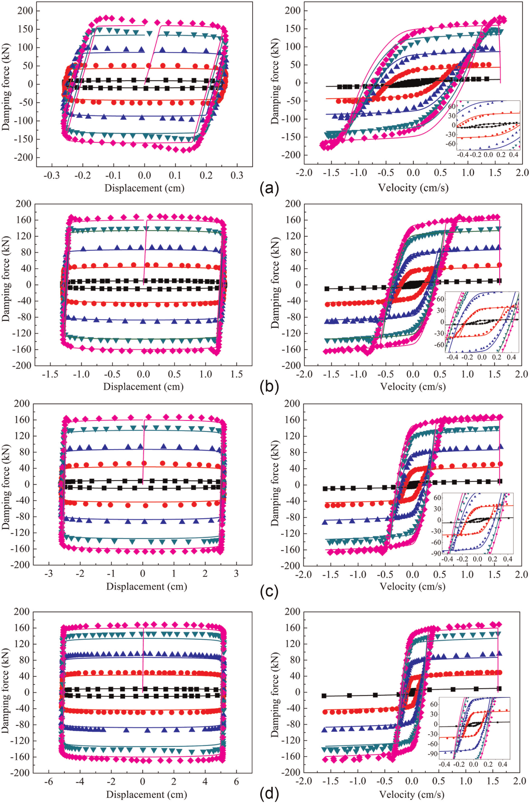
Model predictions (lines) and experimental data (symbols; Yang, 2001) of hysteretic behavior of MR dampers under sinusoidal displacement excitations: (a) 0.254 cm, 1 Hz; (b) 1.27 cm, 0.2 Hz; (c) 2.54 cm, 0.1 Hz; and (d) 5.08 cm, 0.05 Hz.

A feasibility study on modeling the air content effect with the proposed physical model

Before a special MR fluid filling equipment and a pressurized accumulator were used (i.e. P₁(0) = P₂(0) = 0) to reduce the air content, a large air content caused serious force lag in Yang’s (2001) experiment, as shown in Figure 8. Since the proposed model includes the effect of air content, such force lag should be also predicted by the proposed damper model. However, the initial air content before utilizing the pre-pressurized accumulator was not tested in Yang’s (2001) study, so only a qualitative study can be made here on the feasibility of modeling the force lag by a physical model. When a guessed air content of 7% is used, about twice the air content when the chamber is pressurized, the model prediction agrees well with the experimental data in the literature. Thus, the force lag of MR dampers can be captured by including the air content effect in a physical model.

Figure 8.

Model prediction and experimental data (Yang, 2001) of the hysteresis of the damper with unpressurized accumulator (φ₁ = φ₂ = 7%, P₁(0) = P₂(0) = 0, input current = 0.5 A).

A lumped parameter physical model

In fact, if the bulk moduli of the fluid–air mixture in both chambers are assumed to be the same constant independent of the air content and the pressure, that is, e₁ = e₂ = e, then the rate of the change of the damping force can be obtained by subtracting equation (14) from equation (11)

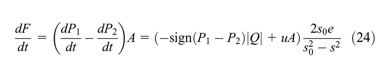
\frac{dF}{dt} = (\frac{d P_{1}}{dt} - \frac{d P_{2}}{dt}) A = (- sign (P_{1} - P_{2}) | Q | + uA) \frac{2 s_{0} e}{s_{0}^{2} - s^{2}}

(24)

After rearrangement, it can be written as

u - \frac{dF / dt}{k} = u_{e}

(25)

where $k = 2 s_{0} eA / (s_{0}^{2} - s^{2}) and u_{e} = sign (P_{1} - P_{2}) | Q | / A$ . It becomes clear that equation (25) is a lumped physical model as shown in Figure 9. The term u_e serves as an effective velocity, which directly generates the flow rate of MR fluid in the gap. The spring (k) represents the compressibility of MR fluid and is equivalent to the oil spring (k_oil) of a hydraulic cylinder (Akers et al., 2006), as shown in Figure 10, which is defined by

k_{oil} = \frac{F_{hydraulic}}{s} = e (\frac{A_{1}^{2}}{V_{1}} + \frac{A_{2}^{2}}{V_{2}}) = e (\frac{A_{1}^{2}}{(s_{0} - s) A_{1}} + \frac{A_{2}^{2}}{(s_{0} + s) A_{2}})

(26)

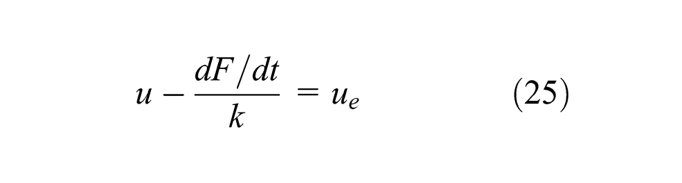
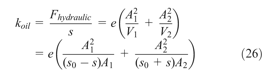
where F_hydraulic is the external driven force, s is the displacement of the piston, e is the bulk modulus of oil–air mixture, A₁ and A₂ are the cross-sectional areas of two chambers, V₁ and V₂ are the volumes of two chambers, and s₀ is the stroke of piston.

Figure 9.

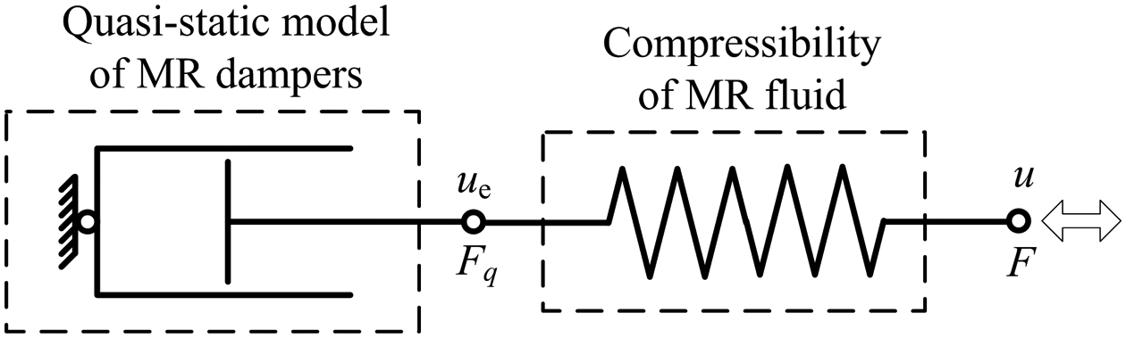
The lumped parameter physical model of MR dampers.

Figure 10.

The oil spring of a hydraulic cylinder.

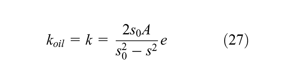
If A₁ = A₂ = A, the hydraulic oil spring (k_oil) is same as the spring (k) in equation (25)

k_{oil} = k = \frac{2 s_{0} A}{s_{0}^{2} - s^{2}} e

(27)

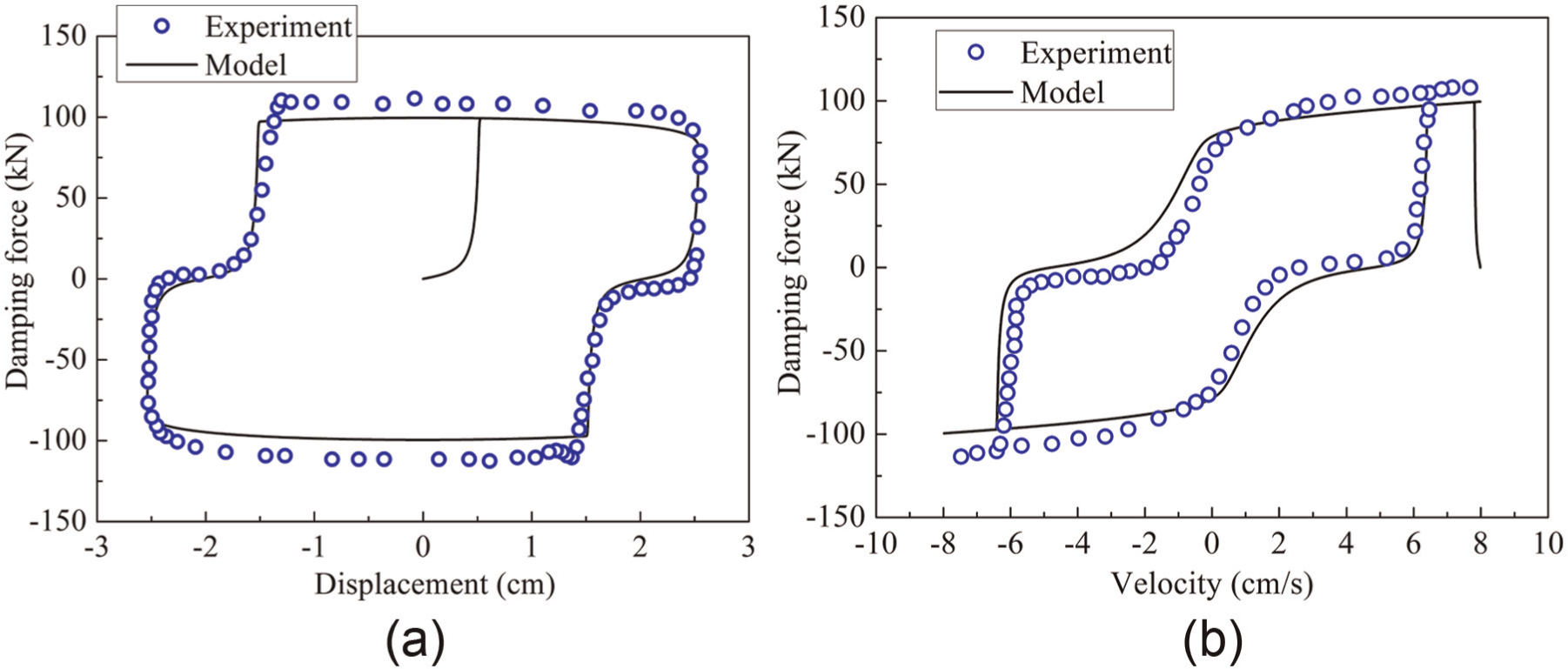
Again, the force–velocity hysteresis of the MR damper in the literature (Yang, 2001) is simulated by the proposed lumped physical model with bulk modulus taken as 0.3 GPa (Batterbee et al., 2007b). The model result shows a good agreement with the testing data, as shown in Figure 11, so the lumped physical model is reliable. It is also worth noting that the value of bulk modulus of the mixture found by Batterbee et al. (2007b), 0.3 GPa, is indeed a good initial estimation for a normally working MR damper, very useful when lacking accurate experimental data.

Figure 11.

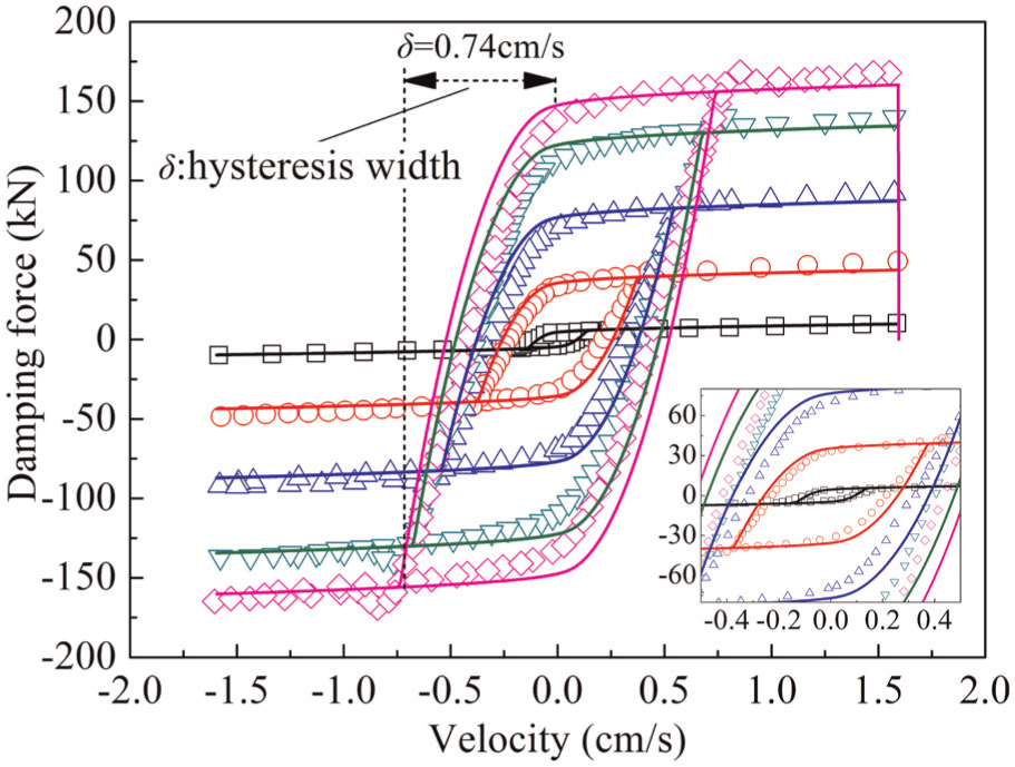
Model prediction and experimental data of the hysteresis behavior of an MR damper (symbols: experimental data (Yang, 2001); lines: prediction; sinusoidal displacement excitation: 1.27 cm and 0.2 Hz; bulk modulus: e = 0.3 GPa).

The most simplified physical model to capture the essence of the hysteresis behavior

Since the damping force of an MR damper is composed of a Coulomb term F_τ and a viscous term F_η, the mechanical model in Figure 9 can be further decomposed to the three basic elements as shown in Figure 12, in which the viscous element and the friction element are connected in parallel, together constituting a quasi-static model.

Figure 12.

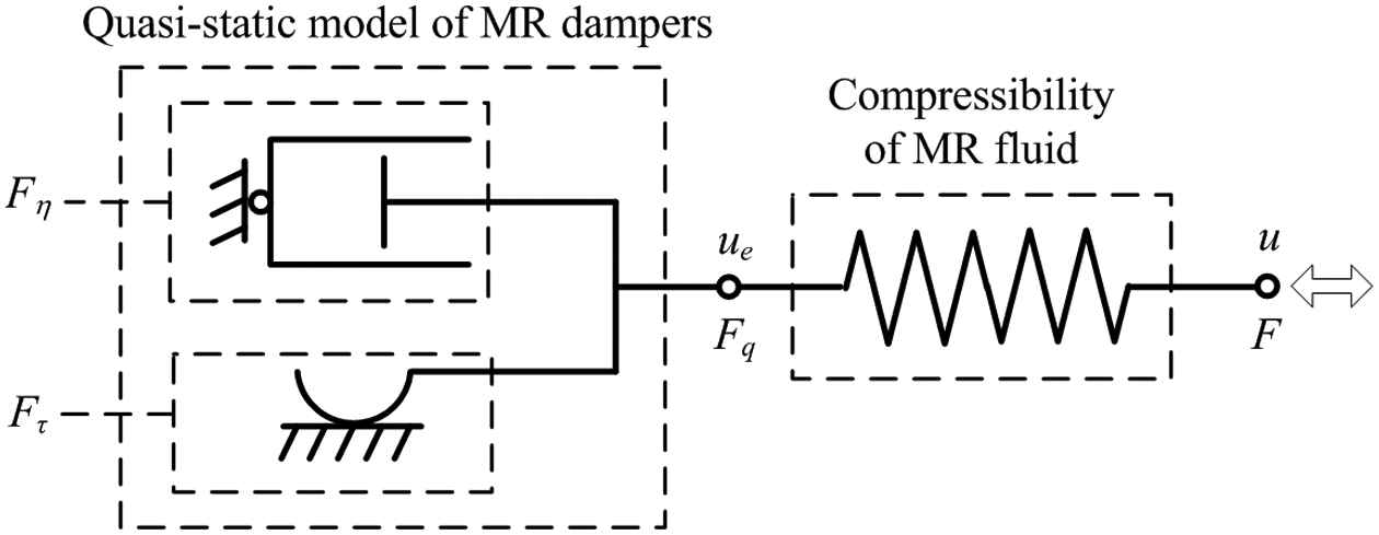
The lumped physical model of MR dampers represented by basic mechanical elements.

A small magnetic field can make freely flowing MR fluid exhibit solid-like characters, and the Coulomb force F_τ of an MR damper is generally several orders of magnitude greater than the viscous force F_η. By ignoring the viscous force term, the lumped physical model would be reduced to its most simplified form as shown in Figure 13.

Figure 13.

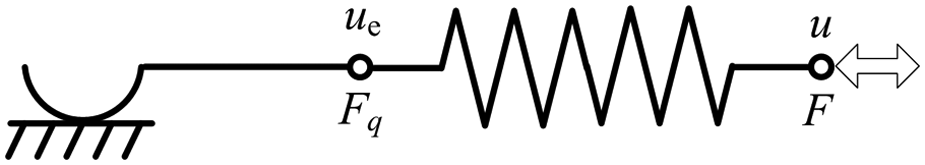
The most simplified lumped parameter physical model of MR dampers.

However, before making this reduction, it is safe to study the viscosity effect on the hysteresis first, and the model in Figure 14 is selected to examine such effect, with the result shown in Figure 15. Apparently, the experimental hysteretic curves in Figure 11 are similar, in shapes, to the curves under low viscosities in Figure 15, so it is reasonable to ignore the viscosity effect. Accordingly, the simplified model should well describe the hysteresis behavior of MR dampers in a more fundamental way, and this is shown in the next section.

Figure 14.

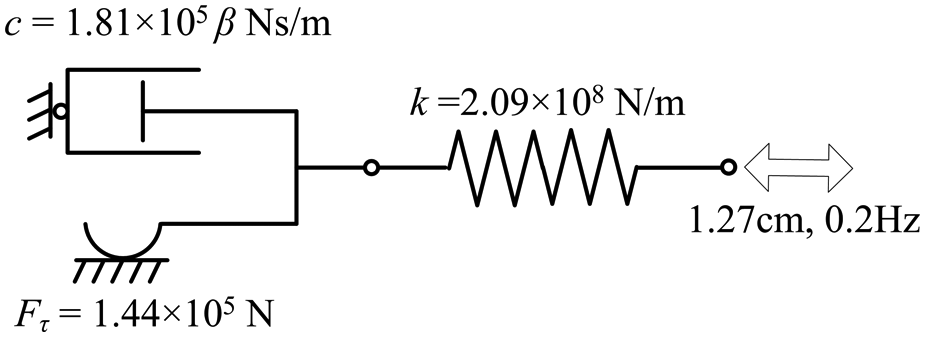
A lumped parameter physical model selected to study the effect of viscosity on the hysteresis.

Figure 15.

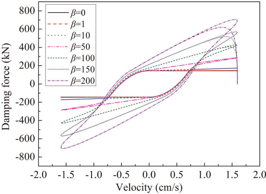
Effect of the viscosity of MR fluid on the force–velocity hysteresis of MR dampers.

The mechanism of the hysteresis generation and the formula for calculating hysteresis width

The mechanism of the hysteresis generation

Undoubtedly, to know the physical process of the hysteresis generation is essential for understanding the dynamic performance of MR dampers, but there has been little such report so far. Utilizing the simplified physical model (Figure 13), the physical process of the hysteresis generation is presented in detail as follows.

In Figure 16, the evolutions of the piston velocity u and the effective velocity u_e are shown together with the corresponding dynamic force F and the quasi-static force F_q during one period of a complete generation process of the hysteresis. The damping force (F) lags far behind the piston velocity (u) when the piston changes its direction, during which the effective velocity (u_e) is even around 0. It is this large force lag that should be responsible for the hysteresis observed in the force–velocity of MR dampers, and a detailed analysis is as below.

Figure 16.

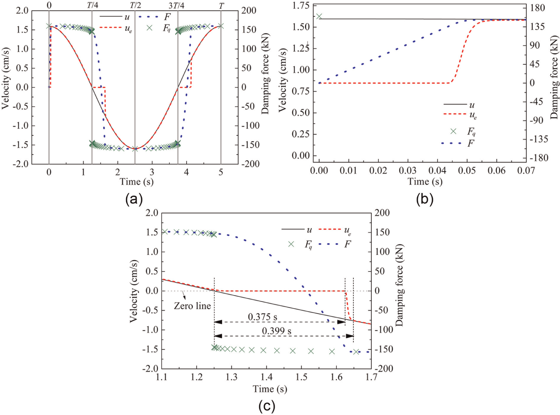
History curves of the piston velocity u, the effective velocity u_e, the dynamic force F, and the quasi-static force F_q during one period of a complete generation process of the hysteresis (1.27 cm, 0.2 Hz, 2 A). (a) Changes of the velocities (u, u_e) and forces (F, F_q) during one whole period, (b) detailed changes of the velocities (u, u_e) and forces (F, F_q) in the first quarter period, and (c) detailed changes of the velocities (u, u_e) and forces (F, F_q) in the second quarter period.

In the first quarter period, the piston starts to move with the maximum velocity, so the damping force F increases to the sliding force F_τ in a relatively short time (about 55 ms, see Figure 16(b)), and the force lag is not evident. During this process, the friction element is kept at rest (u_e = 0), and the damping force is only contributed by the spring force; once the dynamic force exceeds the sliding force, the friction element starts to move and then decelerates together with the spring at nearly the same velocity (u≈u_e) until they stop together.

In the second quarter period, the spring gradually restores to its original length as the piston is returning back from the previous stationary state, and the dynamic force decreases from the sliding force, F_τ, down to 0. The friction element maintains its stationary state all the time in this progress. Then, the further moving back of the piston makes the spring begin to stretch from its original length, and the damping force increases in the opposite direction from 0 up to the sliding force, for example, from 0 to −F_τ. The whole progress, from F_τ to −F_τ, takes a relatively long time (about 400 ms as shown in Figure 16(c)), and the obvious lag of the damping force (F) behind the piston velocity (u) is observed; once the damping force (F) exceeds the friction force (F_τ) in magnitude, the friction element starts to accelerate together with the spring element at the same velocity, until they reach the maximum velocity.

In the whole third quarter period, the friction element and the spring element slow down together, until they stop at the beginning of the next quarter period. In the fourth quarter period, the changes of the velocities and damping force are similar to those in the second quarter period.

The formula for calculating the hysteresis width

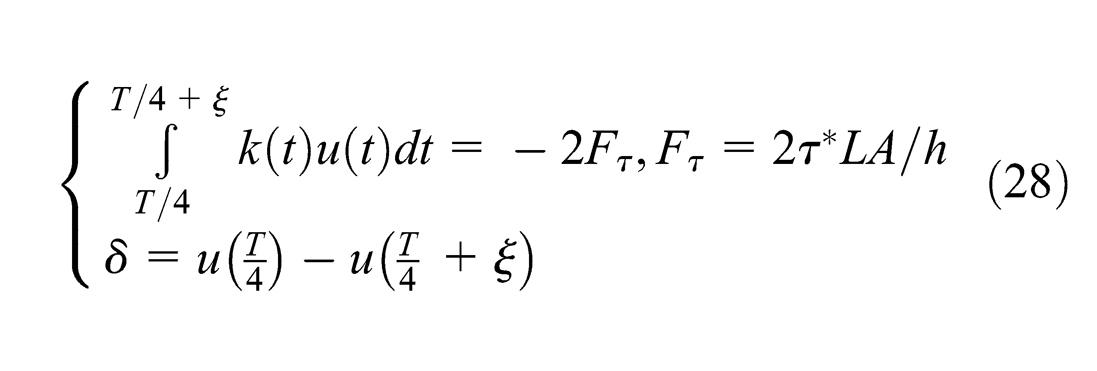
With the understanding of the changes of damping force in the second quarter period of the hysteresis generation, the following equation for calculating the hysteresis width (δ, as shown in Figure 11) is proposed based on the simplified lumped parameter physical model

{\begin{matrix} \int_{T / 4}^{T / 4 + ξ} k (t) u (t) dt = - 2 F_{τ}, F_{τ} = 2 τ^{*} LA / h \\ δ = u (\frac{T}{4}) - u (\frac{T}{4} + ξ) \end{matrix}

(28)

where ξ is the time delay of the damping force behind the piston velocity during the second quarter period of the hysteresis generation.

In the case of 1.27 cm amplitude, 0.2 Hz frequency sinusoidal displacement excitation, and 2 A input current, the time delay (ξ) and the hysteresis width (δ) are obtained by equation (28) as 0.373 s and 0.72 cm/s, which are close to the experimental data 0.375 s in Figure 16(c) and 0.74 cm/s in Figure 11, respectively. Thus, equation (27) is reliable and useful for estimating the hysteresis width.

The hysteresis design of MR dampers

So far, the designs of MR dampers are still the static performance designs based on the quasi-static models in which the damping force and piston velocity always keep synchronous variations, for example, no hysteresis exists. The proposed physical model in this article makes it possible to conduct the hysteresis design of MR dampers, and such design is presented by the following example.

Provided that an MR damper with a stroke of 30 mm (s₀ = 30 mm) is needed, try to design its specific dimensions such that when it works under the sinusoidal displacement excitations of 1 cm and 1 Hz at a constant input current of 1 A, the following design requirements should be fulfilled. For simplicity, the structural parts of this damper can be assumed to be all made of steel with high magnetic permeability.

Static performance requirements. The maximum damping force at the input current of 1 A should be at least 100 kN, and the adjustable ratio when the input current is rising from 0.5 to 1 A should be twice at least.

Dynamic performance requirements. The hysteresis width should be less than the one-fifth of the maximum excitation velocity.

See Figure 17 for the physical meanings of all design variables.

Figure 17.

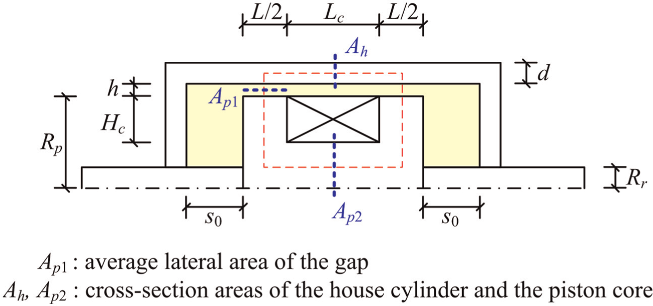
Typical design variables of an MR damper.

As shown in Figure 17, with the stroke (s₀) determined, there are seven other design variables in a typical design of an MR damper, including the thickness of the house cylinder (d), the radius of the piston rod (R_r), the radius of the piston (R_p), the effective length of the piston (L), the gap (h), the coil length (L_c), and the coil height (H_c). The design flow diagram is shown in Figure 18, with the detailed process as follows.

Figure 18.

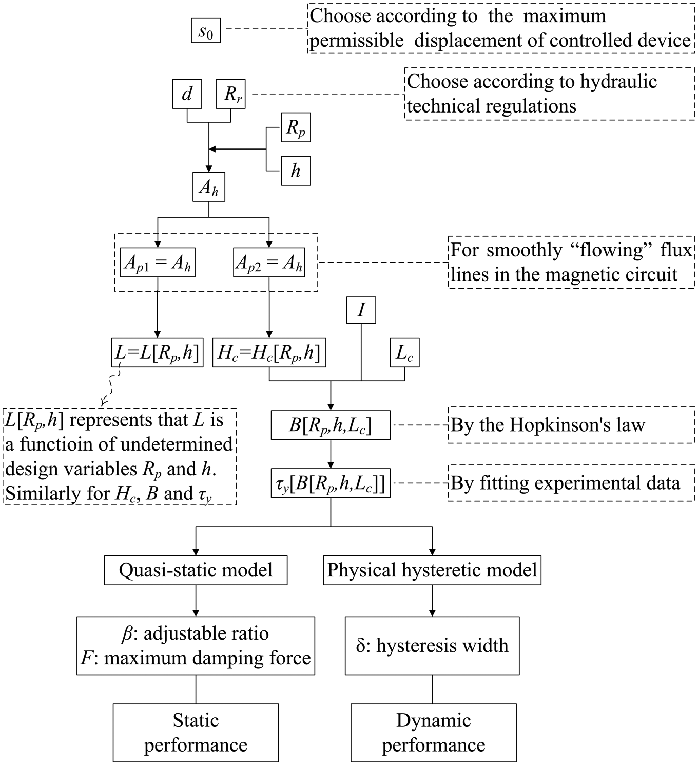
Hysteresis design of MR dampers by fundamentally designing R_p, h, and L_c according to the static and dynamic performance requirements.

The thickness of the house cylinder (d) and the radius of the piston rod (R_r)

Determinations of these two design variables are well documented in hydraulic technical regulations. Basically, the house cylinder should be thick enough so that it can bear the maximum damping force, and the piston rod should have high stability besides the high strength. Here, d and R_r are chosen to be 1 and 2 cm for simplicity.

Magnetic circuit design

The whole magnetic circuit would be saturated, if any part of the circuit gets saturated. Here, the cross-sectional areas of the three major parts of the magnetic circuit (e.g. A_h, A_p₁, and A_p₂ as shown in Figure 17) are chosen to be the same in order to achieve a more smoothly “flowing” flux lines in the circuit

A_{p 1} = A_{p 2} = A_{h}

(29)

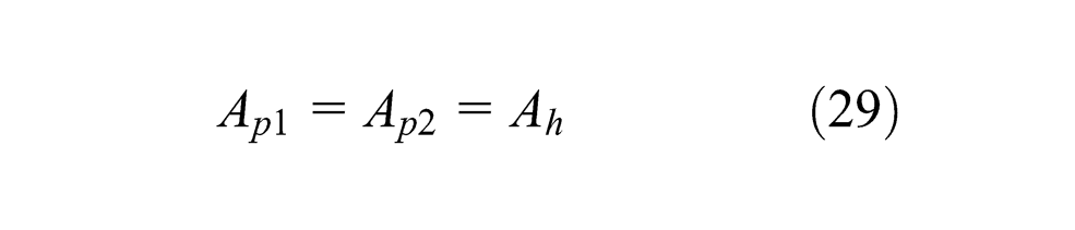
where A_h and A_p₂ are the cross-sectional areas of the house cylinder and the piston core, respectively, and A_p₁ is the average lateral area of the gap, as shown in Figure 17.

In fact, if such choice for design variables is undesirable or impractical, it can still lead to a nontrivial preliminary design and help designers do further modifications. Substituting A_p₁ = 2π(R_p+h/2)(L/2) and A_p₂ = π(R_p−H_c)² into the above equation, then H_c and L are obtained as

{\begin{matrix} H_{c} = R_{p} - \sqrt{\frac{A_{h}}{π}} \\ L = \frac{2 A_{h}}{π (2 R_{p} + h)} \\ A_{h} = π ({(R_{p} + h + d)}^{2} - {(R_{p} + h)}^{2}) \end{matrix}

(30)

Magnetic flux density in the gap

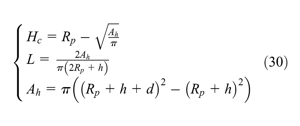
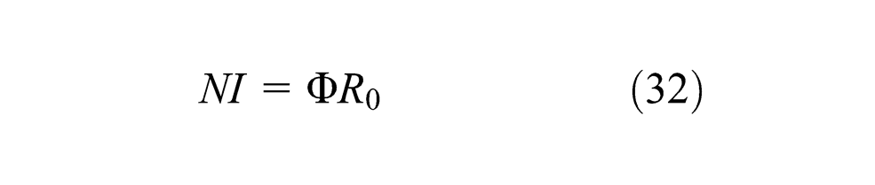
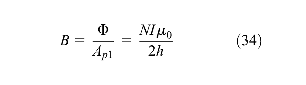
According to Hopkinson’s law, a counterpart to Ohm’s law used in magnetic circuits, the magnetic flux generated in the damper can be related to the coil current by

NI = Φ (R_{0} + R_{m})

(31)

where N is the number of turns of the coil, I is the single-turn current, Φ is the magnetic flux, and R₀ and R_m are, respectively, the magnetic reluctance of the air gap and that of the steel parts constituting the magnetic circuit.

Because $R_{0} >> R_{m}$ , the above equation is reduced to

NI = Φ R_{0}

(32)

As shown in Figure 17, the magnetic reluctance of the gap is

R_{0} = 2 \frac{h}{μ_{0} A_{p 1}}

(33)

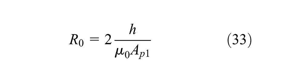
where µ₀ is the magnetic permeability of free space.

By equations (32) and (33), the magnetic flux density in the gap, B, can be written as

B = \frac{Φ}{A_{p 1}} = \frac{NI μ_{0}}{2 h}

(34)

The number of turns of the coil can be estimated according to the dimensions of the coil

N = Floor (k_{N} \frac{L_{c} H_{c}}{π r^{2}})

(35)

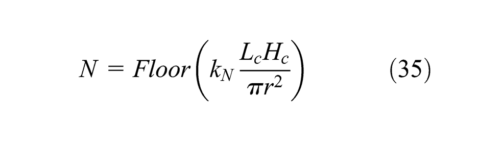
where k_N is the filling factor of the coil and chosen to be 0.97 here and r is the radius of the coil wire and chosen to be 0.5 mm here.

As shown in Figure 19, by fitting the experimental data, the shear yield stress of MR fluid τ is obtained as a function of the magnetic flux density B

τ_{y} = 54830.33 (1 - e^{- 3.14 B^{2.03}})

(36)

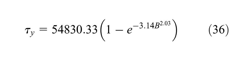
Finally, the shear yield stress actually depends on three design variables, for example, L_c, R_p, and h.

Figure 19.

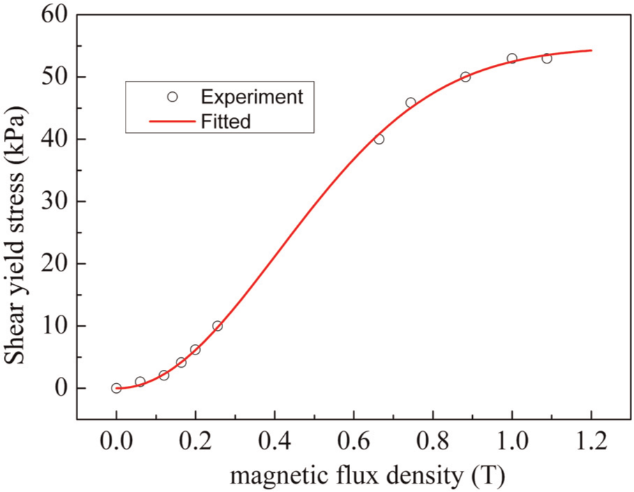
Dependence of shear yield stress of MR fluid on magnetic flux density.

The maximum damping force and the maximum adjustable ratio

The damping force, F, is obtained by numerically solving the following Bingham quasi-static model

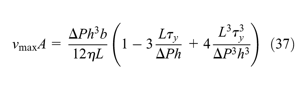
v_{max} A = \frac{Δ P h^{3} b}{12 η L} (1 - 3 \frac{L τ_{y}}{Δ Ph} + 4 \frac{L^{3} τ_{y}^{3}}{Δ P^{3} h^{3}})

(37)

where η is the apparent viscosity of MR fluid and here chosen to be 1.3 Pa s and the maximum velocity, v_max, is 6.28 cm/s in the case of 1 cm and 1 Hz displacement excitation.

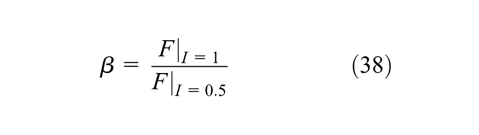
The adjustable ratio can be calculated as the ratio of damping force with 1 A input current to that with 0.5 A current

β = \frac{{F |}_{I = 1}}{{F |}_{I = 0.5}}

(38)

The static performance requirement is mathematically represented by the following inequality system

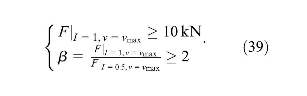
{\begin{cases} {F |}_{I = 1, v = v_{\max}} \geq 10 kN \\ β = \frac{{F |}_{I = 1, v = v_{\max}}}{{F |}_{I = 0.5, v = v_{\max}}} \geq 2 \end{cases} .

(39)

The feasible region represented by equation (39) is numerically solved in Mathematica software, with the result shown in Figure 20(a).

Figure 20.

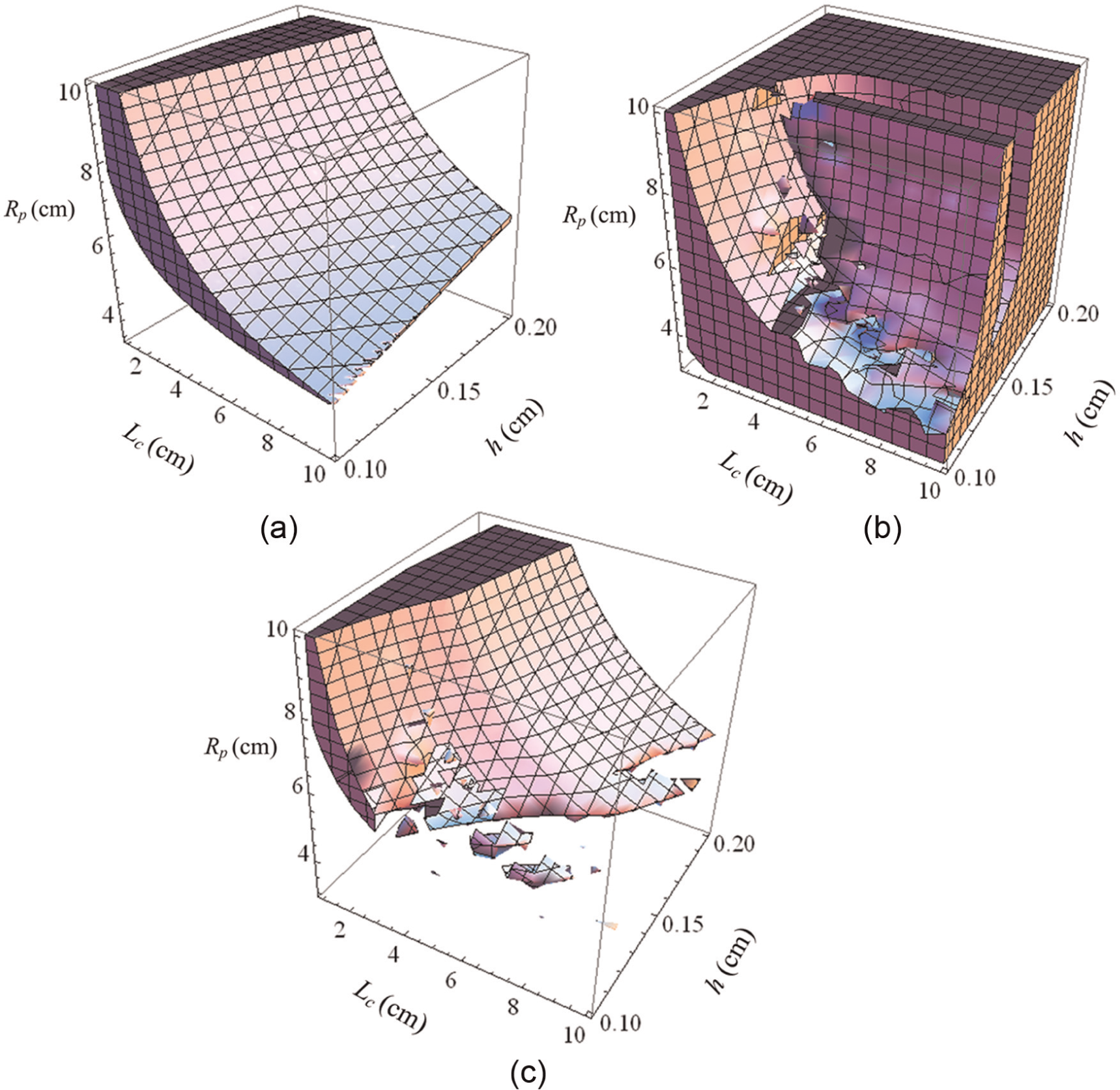
Dynamic design of an MR damper: (a) feasible design region satisfying the damping force requirement, (b) feasible design region satisfying the hysteresis width requirement and (c) feasible design region satisfying both the force demands and the hysteresis width demands.

The hysteresis width

The dynamic performance requirement corresponds to the following inequality

δ \leq \frac{v_{max}}{5}

(40)

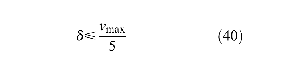
With equation (28), inequality (40) is solved in Mathematica software, and the feasible region is shown in Figure 20(b).

Actually, the inequality system consisting of equations (39) and (40) can be solved together in Mathematica software, but the consumption time is much longer than that of solving inequalities separately. The feasible region of this inequality system is shown in Figure 20(c), which is the intersection of the two regions in Figure 20(a) and (b).

Selection of feasible design variables and design validation

According to the feasible region shown in Figure 20(c), this damper is finally designed as R_p = 80 mm, L_c = 40 mm, and h = 2 mm, and the other design variables L, H_c, B, and τ_y can be calculated as 21.48 mm, 38.29 mm, 0.594 T, and 35.67 kPa. Then, the static and dynamic performances of the designed damper are computed by the Bingham model and the proposed simplified physical model, respectively, with the result shown in Figure 21. The designed maximum damping force is 23 kN, the maximum adjustable ratio is 10.6, and the hysteresis width is about 12% of the maximum velocity for the designed damper, so all the design requirements are satisfied.

Figure 21.

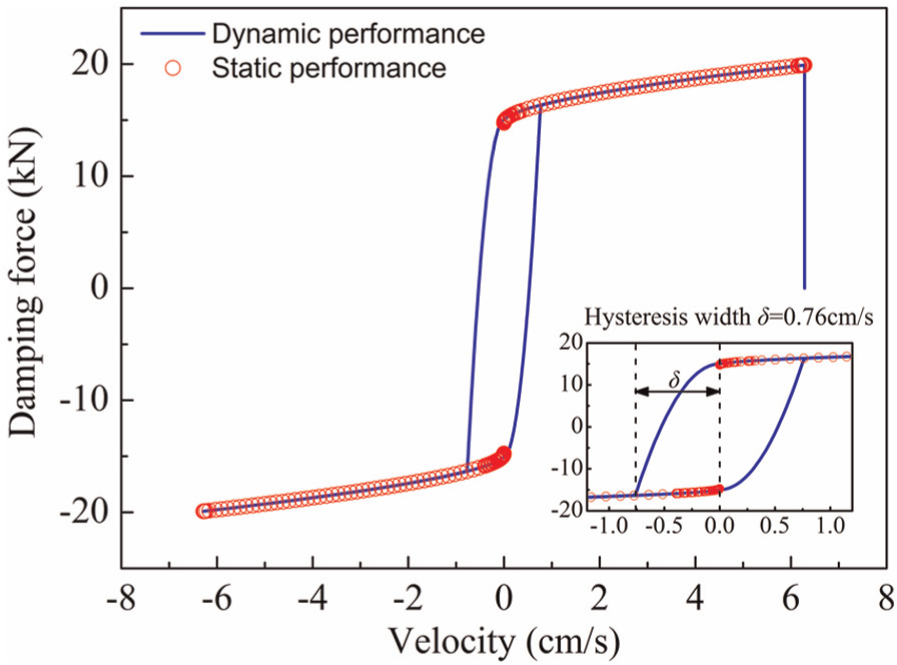
The static and dynamic performances of the designed MR damper.

Conclusion

A physical model is developed by combining the compressibility of MR fluid with a general quasi-static model in this article, which can well describe, in an essential physical way rather than the popular phenomenological way, the hysteresis behavior of MR dampers, and the description becomes more elaborate by including the air content effect. Ignoring such air content and assuming that the compressibility of fluid–air mixture is independent of the pressure, an equivalent lumped parameter physical model with clear physical meaning is derived and also proven to have an equivalent capability of describing the hysteresis behavior. Generally, the viscous force can be ignored in comparison with the Coulomb force, and this fact leads to the most simplified hysteretic physical model in which a friction element representing the Coulomb force is connected in series with a spring element representing the compressibility of fluid. Based on this simplified physical model, the physical process (or the mechanism) of the hysteresis generation is explored in great detail. Besides, the formula for calculating the hysteresis width is proposed, which makes the hysteresis design possible, and such design method is also presented by an example.

Footnotes

Funding

This research is financially supported by the National Natural Science Foundation of China under grant 90815027, Program of Ministry of Transport of China under grant 2011318494180, National Key Technology R&D Program of China under grant 2011BAK02B01, and Program for New Century Excellent Talents in University under grant NCET-10-0056.

References

Akers

Gassman

Smith

(2006) Hydraulic Power System Analysis. New York: Taylor & Francis Group.

Akkaya

(2006) Effect of bulk modulus on performance of a hydrostatic transmission control system. Sadhana 31(5): 543–556.

Ali

Ramaswamy

(2009) Hybrid structural control using magnetorheological dampers for base isolated structures. Smart Materials and Structures 18(5): 1–16.

Batterbee

Sims

Stanway

. (2007a) Magnetorheological landing gear: 1. A design methodology. Smart Materials and Structures 16(6): 2429–2440.

Batterbee

Sims

Stanway

. (2007b) Magnetorheological landing gear: 2. Validation using experimental data. Smart Materials and Structures 16(6): 2441–2452.

Bhatnagar

(2013) Transient effect modelling of magnetorheological fluid-based damper at low speed and its comparison with the existing magnetorheological damper models. Journal of Intelligent Material Systems and Structures. Epub ahead of print 28 January. DOI: 10.1177/1045389X12474355.

Chang

Roschke

(1998) Neural network modeling of a magnetorheological damper. Journal of Intelligent Material Systems and Structures 9(9): 755–764.

Chang

Zhou

(2002) Neural network emulation of inverse dynamics for a magnetorheological damper. Journal of Structural Engineering 128(2): 231–239.

Choi

Lee

Park

(2001) A hysteresis model for the field-dependent damping force of a magnetorheological damper. Journal of Sound Vibration 245(2): 375–383.

10.

Lam

Zhang

(2006) Modelling of a magneto-rheological damper by evolving radial basis function networks. Engineering Applications of Artificial Intelligence 19(8): 869–881.

11.

Dyke

Spencer

Jr Sain

. (1999) Modeling and control of magnetorheological dampers for seismic response reduction. Smart Materials and Structures 5(5): 565–575.

12.

Gavin

Hanson

Filisko

(1996) Electrorheological dampers, part II: testing and modeling. Journal of Applied Mechanics 63(3): 676–682.

13.

Giorgetti

Baldanzini

Biasiotto

. (2010) Design and testing of a MRF rotational damper for vehicle applications. Smart Materials and Structures 19(6): 065006.

14.

Goldasz

Sapinski

(2013) Verification of magnetorheological shock absorber models with various piston configurations. Journal of Intelligent Material Systems and Structures. Epub ahead of print 15 March. DOI: 10.1177/1045389X13479684.

15.

Gordaninejad

Kelso

(2000) Fail-safe magneto-rheological fluid dampers for off-highway, high-payload vehicles. Journal of Intelligent Material Systems and Structures 11(5): 395–406.

16.

Guan

Guo

(2011) Modeling of magnetorheological dampers utilizing a general nonlinear model. Journal of Intelligent Material Systems and Structures 22(5): 435–442.

17.

Hong

Choi

. (2005) A hydro-mechanical model for hysteretic damping force prediction of ER damper: experimental verification. Journal of Sound and Vibration 285(4): 1180–1188.

18.

Hong

John

Wereley

. (2008) A unifying perspective on the quasi-steady analysis of magnetorheological dampers. Journal of Intelligent Material Systems and Structures 19(8): 959–976.

19.

Kamath

Wereley

(1997) Nonlinear viscoelastic-plastic mechanism-based model of an electrorheological damper. Journal of Guidance, Control and Dynamics 20(6): 1125–1132.

20.

Lee

Choi

Wereley

(2002) Performance analysis of ER/MR impact damper systems using Herschel-Bulkley model. Journal of Intelligent Material Systems and Structures 13(7–8): 525–531.

21.

Lee

Nam

Yamane

. (2009) Performance evaluation on vibration control of MR landing gear. Journal of Physics Conference Series 149(1): 012068.

22.

Wang

Rakheja

. (2002) Modeling hysteretic characteristics of MR fluid damper and model validation. In: Proceedings of the 41st IEEE conference on decision and control, vol. 2, Las Vegas, NV, 10–13 December, pp. 1675–1680. New York: IEEE.

23.

Peel

Stanway

Bullough

(1996) Dynamic modeling of an ER vibration damper for vehicle suspension applications. Smart Materials and Structures 5(5): 591–606.

24.

Phillips

(1969) Engineering applications of fluids with a variable yield stress. PhD Thesis, University of California, Berkeley, CA.

25.

Şahin

Engin

Çeşmeci

(2010) Comparison of some existing parametric models for magnetorheological fluid dampers. Smart Materials and Structures 19(3): 035012.

26.

Sassi

Cherif

Mezghani

. (2005) An innovative magnetorheological damper for automotive suspension: from design to experimental characterization. Smart Materials and Structures 14(4): 811–822.

27.

Schurter

Roschke

(2000) Fuzzy modeling of a magnetorheological damper using ANFIS. In: The ninth IEEE international conference on fuzzy systems, vol. 1, San Antonio, TX, 7–10 May, pp. 122–127. New York: IEEE.

28.

Sims

Stanway

Peel

. (1999) Controllable viscous damping: an experimental study of an electrorheological long-stroke damper under proportional feedback control. Smart Materials and Structures 8(5): 601–615.

29.

Spencer

Jr Dyke

Sain

. (1997) Phenomenological model for magnetorheological dampers. Journal of Engineering Mechanics: ASCE 123(3): 230–238.

30.

Wang

Liao

(2004) Modeling and control of magnetorheological fluid dampers using neural networks. Smart Materials and Structures 14(1): 111–126.

31.

Wang

Liao

(2011) Magnetorheological fluid dampers: a review of parametric modelling. Smart Materials and Structures 20(2): 023001.

32.

Wang

Faramarz

(1999) Flow analysis of field-controllable, electro- and magneto-rheological fluids using Herschel-Bulkley model. Journal of Intelligent Material Systems and Structures 10(8): 601–608.

33.

Wang

Faramarz

(2007) Flow analysis and modeling of field-controllable, electro- and magneto-rheological fluid dampers. Journal of Applied Mechanics 74(1): 13–22.

34.

Wereley

(2008) Nondimensional Herschel-Bulkley analysis of magnetorheological and electrorheological dampers. Journal of Intelligent Material Systems and Structures 19(3): 257–268.

35.

Wereley

Lindler

Rosenfeld

. (2004) Biviscous damping behavior in electrorheological shock absorbers. Smart Materials and Structures 13(4): 743–752.

36.

Wereley

Pang

Kamath

(1998) Idealized hysteresis modeling of electrorheological and magnetorheological dampers. Journal of Intelligent Material Systems and Structures 9(8): 642–649.

37.

Wilson

CMD

Abdullah

(2005) Structural Vibration Reduction Using Fuzzy Control of Magnetorheological Dampers. New York: ASCE Structures Congress.

38.

Yang

(2001) Large-scale magnetorheological fluid damper for vibration mitigation: modeling, testing and control. PhD Thesis, University of Notre Dame, Notre Dame, IN.

39.

Zhou

Nielsen

SRK

(2006) Semi-active control of three-dimensional vibrations of an inclined sag cable with magnetorheological dampers. Journal of Sound and Vibration 296(1): 1–22.

Physical modeling and design method of the hysteretic behavior of magnetorheological dampers

Abstract

Keywords

Introduction

Quasi-static models: modeling and designing damping force of MR dampers operated at constant piston velocities

A physical hysteretic model of MR dampers

Flow rate equation based on the compressibility of fluid

Compressibility of air–fluid mixture in the chamber

Validation of the proposed physical model

A feasibility study on modeling the air content effect with the proposed physical model

A lumped parameter physical model

The most simplified physical model to capture the essence of the hysteresis behavior

The mechanism of the hysteresis generation and the formula for calculating hysteresis width

The mechanism of the hysteresis generation

The formula for calculating the hysteresis width

The hysteresis design of MR dampers

The thickness of the house cylinder (d) and the radius of the piston rod (Rr)

Magnetic circuit design

Magnetic flux density in the gap

The maximum damping force and the maximum adjustable ratio

The hysteresis width

Selection of feasible design variables and design validation

Conclusion

Footnotes

Funding

References

The thickness of the house cylinder (d) and the radius of the piston rod (R_r)