
Abstract
We investigate a new approach for characterizing class separability based on topological measures for use with identifying flaw severity in plates. Multi-mode Lamb waves are propagated across a flat-bottom hole of varying depth. Lamb wave tomography reconstructions are first generated to locate and size the flaw at each depth. As the flaw depth increases, scattering and mode conversion effects dominate the raw time-domain signals, obscuring information about flaw severity. Pattern classification provides an alternate means for processing the ultrasonic waveforms to identify flaw severity. High-dimensional feature spaces are generated from the Lamb wave signals using the dynamic wavelet fingerprinting technique. In order to achieve high classification accuracy, an optimal feature space is required. An intelligent feature selection routine is explored here that identifies favorable class distributions in multidimensional feature spaces using computational homology theory. Betti numbers and formal classification accuracies are calculated for each feature space subset to establish a correlation between the topology of the class distribution and the corresponding classification accuracy.
Introduction
Lamb waves are a promising structural health monitoring (SHM) technique due to their through-thickness multi-mode propagation (Raghavan and Cesnik, 2007; Rose, 2002). Lamb waves are confined by a structure’s boundaries, giving sensitivity to material discontinuities at both surfaces and in the interior of thin materials including plates and pipes (Advani et al., 2010; Giurgiutiu and Cuc, 2005; Pruell et al., 2009; Yu and Giurgiutiu, 2008). Lamb waves also propagate long distances (Alleyne et al., 2009; Carandente and Cawley, 2012) and beneath material coatings (Hinders and Bingham, 2010) allowing for rapid inspection of large areas. Lamb waves provide a useful tool for interrogating structural defects in plates because the group velocity of individual Lamb wave modes is determined by the product of material thickness and transducer frequency used. Their multi-mode structure is often too complex for direct interpretation since high-frequency-thickness values give rise to multiple Lamb wave modes, often with overlapping group velocities (Leckey et al., 2012).
Many SHM applications of guided waves sidestep the complexities of multi-mode signals in some manner. Rather than attempting direct interpretation, one popular approach involves signal comparison with a damage-free baseline measurement to identify changes in a material over time (Wang et al., 2010). This approach is often impractical for use in real-world situations, where environmental and operational conditions result in deviations from the baseline data, which require corrections that may be larger than the waveform distortion caused by the flaw. Another common restriction is to use low-frequency-thickness values for inspection, reducing the number of Lamb wave modes that propagate (Raghavan and Cesnik, 2007). Low-frequency-thickness regimes promise easier analysis of mode arrival-time shifts, as lower order modes tend to be spread apart in group velocity (Bingham and Hinders, 2009). Since each mode propagates with a unique displacement/stress profile (Rose, 1999), it is still beneficial to use multi-mode Lamb wave signals where each mode is sensitive to different defects and has different dispersion characteristics (Leonard, 2005).
Using signals that contain higher order Lamb wave modes requires advanced analysis techniques in order to harness the complex multi-modal behavior. Lamb wave tomography (LWT) can produce quantitative maps of flaws using both single-mode and multi-mode Lamb wave signals (Hou et al., 2004; Leonard et al., 2002; Leonard and Hinders, 2005). By extracting Lamb wave mode arrival times, a slowness map is generated that highlights changes in mode speed that relate to material changes in the plate. These LWT reconstructions provide accurate location and sizing of defects (Hinders et al., 2002). Recent work has resulted in several novel reconstruction techniques that reduce the computational requirements and/or number of transducers required to accurately map an area (Morii et al., 2011; Zhao et al., 2011). Due to overlapping group/phase velocities, however, a direct correlation between mode arrival time and material thickness may not always exist for multi-mode Lamb wave signals. Additional complexities are introduced by more severe defects, where scattering and mode conversion effects dominate the received waveforms. Several techniques have been explored to analyze these strongly scattering defects (Cegla et al., 2008; Diligent et al., 2002; Kim et al., 2010; McKeon and Hinders, 1999; Malyarenko and Hinders, 2001; Moreau et al., 2011, 2012), including Mindlin plate theory approximations (Cegla et al., 2008; McKeon and Hinders, 1999), diffraction tomography (Malyarenko and Hinders, 2001), and using specific transducer polarizations to identify mode conversion effects (Kim et al., 2010).
While LWT reconstructions do not always provide information on flaw severity, they are able to locate and size even strongly scattering flaws. This provides a mechanism to automatically identify the subset of waveforms that have interacted with the material defect present. Pattern classification (Bishop, 2006; Duda et al., 2001) then provides an alternative method to associate features of these waveforms with flaw depth. Statistical pattern classification algorithms generate decision boundaries in a multidimensional feature space based on given training data. New data are then assigned class labels based on their position in the feature space relative to these boundaries. In most applications of pattern classification, each set of objects with a common shared quality is grouped into an individual class. High class separability in the feature space is required if unknown data are to be accurately assigned a class label, but the distribution of individual classes within a feature space is often irrelevant.
Corrosion is a continuous gradual destruction of material where the severity increases with time. Discretizing this continuous material loss into individual flaw depth bins allows each depth to be assigned a unique class label. It is not practical to imagine a training set that includes all possible flaw depths, let alone all possible flaw shapes, positions, and so on. It is therefore highly unlikely that any new data will belong to an existing class of a training set. Rather, it will almost always fall between existing classes and should be labeled as one of these existing class bounds. It follows that the class distribution within a feature space should be sequential with respect to flaw severity, where one class borders the next as flaw severity is increased. An interpolation of sequential classes could recreate the continuous class distribution associated with corrosion.
Reducing a large feature space to only those features that result in sequential class distribution is a feature selection problem. Appropriate features are usually unknown a priori, and as a result, many features are generated without any knowledge of their relevancy (Blum and Langley, 1997). There are three general techniques for feature selection: wrapper methods, embedded methods, and filter methods (Saeys et al., 2007). Wrapper methods use formal classification to rank individual feature space subsets, applying an iterative search procedure that trains and tests a classifier using different feature subsets for accuracy comparison. This continues until a given stopping criterion is met (Dash and Liu, 1997). This approach is computationally intensive, and there is often a trade-off among algorithms between computation speed and the quality of results that are produced (Fan and Lv, 2010; Guyon and Elisseeff, 2003; Raymer et al., 2000). Additionally, these methods have a tendency to overtrain themselves, where data in the training set are perfectly fitted and result in poor generalization performance (Romero et al., 2003). Similar to wrapper methods, embedded methods perform feature selection while constructing the classification algorithm itself. The difference is that the feature search is intelligently guided by the learning process itself. Filter methods perform their feature ranking by looking at intrinsic properties of the data, without the input of a formal classification algorithm. Traditionally, these methods are univariate and therefore do not account for multifeature dependencies.
Our research explores a new approach to the problem of intelligent feature space reduction. By constructing a representative data set of waveforms that have interacted with a flaw ranging in severity, we seek to identify a feature space where the class distribution is both well separated and sequential. Our feature selection approach can be most appropriately considered a multivariate filter method, as it considers features in combination with each other and does not directly depend on the classification model used. A main difference here is that we redefine what it means for a feature to be “relevant.” Typically, relevant features are identified by their contribution toward class separability. While still important, we add a requirement that the features in combination must result in sequential class connectedness. Here, optimal subsets of a high-dimensional feature space are selected based on topological measurements of the class distribution within the feature space itself. We explore the topological structure of the class distribution in the feature space using computational homology. Specifically, we are trying to find a correlation between topological connectedness of multiclass feature space distributions and their corresponding classification accuracy.
Computational homology has been previously implemented in a variety of analysis applications. Hyde et al. (1995) generated isosurface reconstructions of the atomic structure of thermally treated alloys, identifying a correlation between the number of cavities in each surface and the amount of thermal aging undergone by the alloy. More recent implementations span a range of applications including image processing and recognition (Allili et al., 2001; Niethammer et al., 2002; Zelawski, 2005; Ziou and Allili, 2002), sensor network analysis (De Silva and Ghrist, 2006), material science (Teramoto and Nishiura, 2010), biomedical analysis (Mrozek et al., 2012), and image-based pattern classification (Gameiro et al., 2005; Gameiro and Pilarczyk, 2007). The majority of current applications of computational homology in the sciences revolve around the analysis of 1-dimensional (1D), 2-dimensional (2D), or 3-dimensional (3D) spaces, most commonly in image analysis. We intend to break this mold by using the same algorithms to analyze high-dimensional data sets for favorable class separability.
Our work builds on that of Leonard et al. (2002), where the inverse problem of LWT is solved to provide a technique used to locate and size flaws in plates. Additionally, we build on the preliminary work of Miller and Hinders (2013), where tomography is used in combination with formal pattern classification techniques to attempt to characterize flaw severity. Our analysis explores the use of powerful computational homology algorithms toward a general solution to the inverse problem of damage characterization, where damage-scattered Lamb waves are used to quantify the flaw severity.
Cubical homology
Computational homology is a field of mathematics involving the application of homology theory to geometric data sets generated from physical measurements. We consider a specific implementation of this theory that requires the topological spaces under consideration to be built out of d-dimensional unit cubes with indices on the integer lattice (Kaczynski et al., 2004). This cubical structure extends neatly to experimental data sets, where d-dimensional data sets can be represented as d-dimensional rectangles whose width is determined by some measure of error bounds in each dimension. Recent algorithm development under this cubical set constraint has led to an increase in the application of computational homology for experimental data analysis (Mrozek and Batko, 2009; Mrozek et al., 2008; Peltier et al., 2007).
We seek to generate a quantitative measure of how much overlap exists for a multiclass distribution in a d-dimensional feature space. Homology theory provides us a definitive measure of n-dimensional connectedness for
The mathematical tools used here are not novel. Rather, we present a unique application of them in the context of feature selection. Several publicly available software packages exist for the computation of homologies and their Betti numbers, including Computational Homology Project (CHomP, 2012), the GAP homology package (Dumas et al., 2008), JavaPlex (Tausz et al., 2011), Dionysus (Morozov, 2012), and the RedHom library (Institute of Computer Science at Jagiellonian University, 2012). In our analysis, we use the software CHomP. This software allows for the rapid computation of homology groups based on input of elementary cubical complexes. Specifically, the algorithm used here computes the homologies over the ring of integers.
A simple example of how Betti numbers correlate to the spatial distribution of classes within a feature space is presented in Figure 1. Here, three objects represented as squares are presented in a 2D space for three different levels of overlap: no overlap, slight overlap, and severe overlap. Each object can be thought of as a bounding box representation of an individual class. Because this space is 2D,
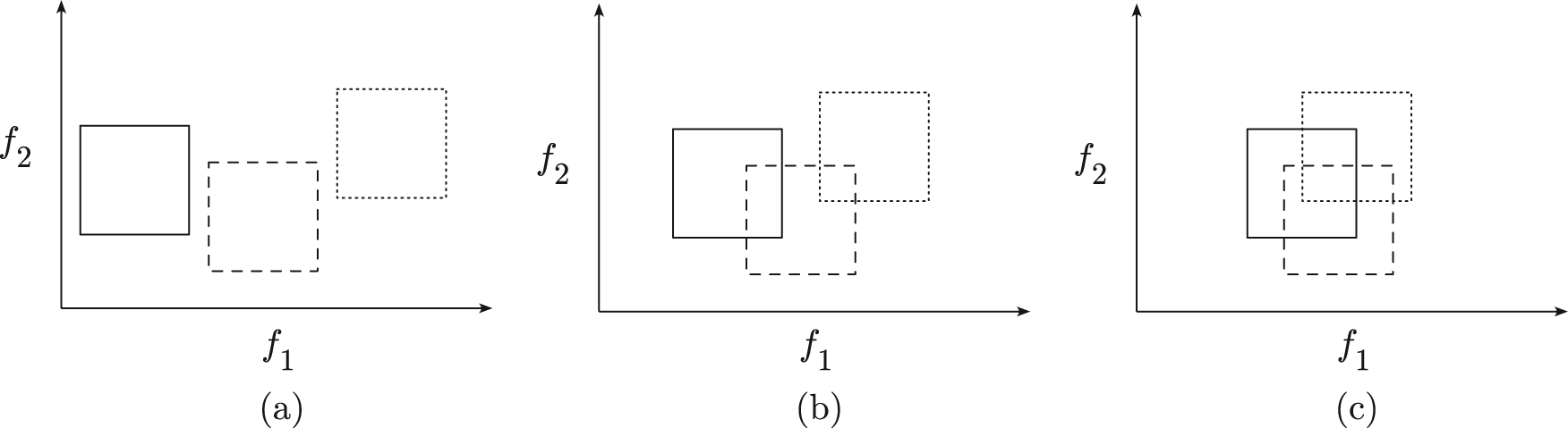
Three objects (classes) in a two-dimensional feature space (
Experimental setup
The data used in this study are collected from a 305 mm × 305 mm × 3.15 mm aluminum plate. A shallow, rounded rectangle void 76 mm in length and 30 mm in width is introduced and then incrementally increased in depth by milling (Miller and Hinders, 2013). Waveforms are transmitted and received using two 2.15-MHz, 6.4-mm-diameter contact transducers in a pitch-catch configuration. The transmitter is excited by a Matec TB1000 tone-burst card, generating a five-cycle sine wave at 2.15 MHz. The received signal is amplified by the Matec card and then digitized using a GaGe CS8012A analog-to-digital (A/D) card. Each transducer is fit with an 11.5-mm-diameter acrylic delay line using a glycerin couplant at both the transducer and the plate surface.
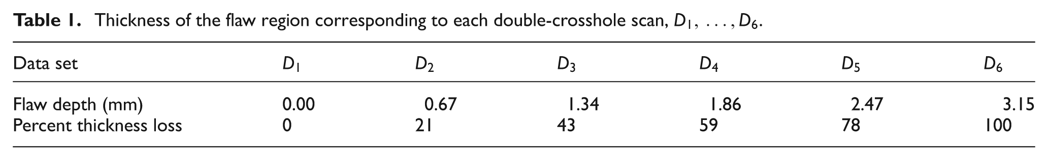
The transducers are stepped individually about the perimeter of a region of interest in a double-crosshole geometry (Leonard et al., 2002), mimicking a four-legged array of transducers surrounding an area of interest. Each transducer is attached to a linear slide, and movement through 100 locations at 2 mm per step is controlled by a Velmex VP9000 motion controller. The transmitter is advanced one position along a particular edge of the region of interest, while the receiver is stepped through all positions on the opposing edge. The transmitter is then advanced to the next position, and the receiver again steps through all positions on the opposing edge. Each projection uses a set of 1002 individual waveforms, with two projections per full scan. A full double-crosshole scan is collected at six flaw depths
Thickness of the flaw region corresponding to each double-crosshole scan,
The group velocity dispersion curve for aluminum is shown in Figure 2, with the frequency–thickness product of the full plate thickness identified by a dotted vertical line at 6.78 MHz mm. Most of the propagating modes at this frequency–thickness have group velocities that are very close together. In addition, the slower
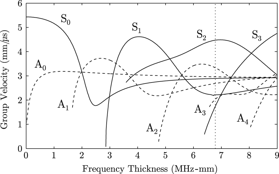
Group velocity dispersion curve for aluminum, with symmetric (solid black line) and antisymmetric (dashed black line) modes shown. Using a 2.15-MHz inspection frequency and a 3.16-mm plate thickness results in a frequency–thickness product of 6.78 MHz mm, highlighted by the black vertical dotted line. This frequency–thickness product is above the cutoff value for multiple modes (
A typical multi-mode waveform is shown in Figure 3, with predicted mode arrival times highlighted. For shallow flaws, changes in the fastest
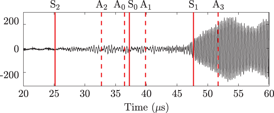
A raw waveform from the unflawed plate is shown here with predicted mode arrival times, indicated for both symmetric (solid vertical lines) and antisymmetric modes (dashed vertical lines). The portion of the signal that is of interest often lies buried in noise (from 25 to 45 µs here), while the higher amplitude portion of the signal (45–60 µs) contains an overlap of both slower, low-velocity modes and faster edge-reflected modes due to the finite size of the plate sample. For the deeper flaw, mode conversion and scattering effects prevent an accurate prediction of arrival times in addition to reducing the signal-to-noise ratio of the waveform.
LWT
Tomographic reconstructions are generated for each class
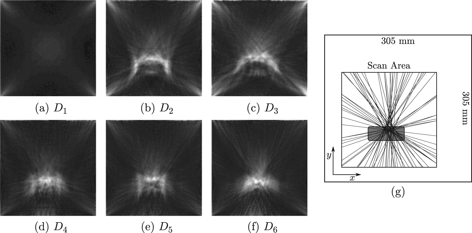
Tomographic reconstructions for classes: (a)
Due to the computation time required to perform feature extraction, the complete set of flaw-only raypaths is reduced further by selecting 50 of these raypaths at random. A visualization of the raypaths selected can be seen overlaid in the scan area seen in Figure 4(g). This random selection is used to minimize geometric bias that could be associated with the shape of the specific flaw used in the training set. Individual waveforms corresponding to these raypaths are identified from each full double-crosshole scan, compiling a data set to use for classification. A total of 300 waveforms are therefore included in the final data set. Individual waveforms are denoted
Feature extraction techniques
Several different methods are used to extract feature values from each of the 300 waveforms: higher order statistics, Mellin transform statistics, wavelet packet decomposition, and dynamic wavelet fingerprinting (DWFP). All these methods provide a specific set of values that have direct physical relation back to the raw data, and each has shown promise in various applications for damage detection (Bertoncini et al., 2012; Bingham and Hinders, 2010; Harley et al., 2012; Mattson and Pandit, 2006; Sun and Chang, 2002). In total, 78 individual features are extracted from each waveform in our data set, resulting in a
Several statistical features commonly used in ultrasonic signal analysis are generated from the raw waveforms (Cox and Hinkley, 1979). Standard time-domain features include the mean of the raw waveform, the variance, the Shannon entropy, the second central moment, the skewness, and the kurtosis of each waveform. Statistical moments provide insight by highlighting outliers due to any specific flaw-type signatures found in the data.
The Mellin transform is an integral transform closely related to the Fourier transform that can represent a signal in terms of a physical attribute similar to frequency known as scale. This transform has the key property of scale invariance. Small variations in mode velocity due to environmental changes, such as temperature fluctuations or applied strain, can be approximated as a uniform time-scaling effect on the transmitted signals. By considering the Mellin domain, features can be compared that are robust to environmental effects. While there are complexities associated with discretizing the fast Mellin transform algorithm, a MATLAB-based implementation is used (De Sena and Rocchesso, 2007). Once the Mellin transform is computed, features are extracted from the resulting Mellin domain for classification. These features include the mean of the Mellin transform, as well as the standard deviation (SD), variance, second central moment, Shannon entropy, kurtosis, and skewness of the mean-removed Mellin transform (Harley et al., 2012).
In the DWFP technique (Hou and Hinders, 2002), a continuous wavelet transform is applied to each of the original time-domain waveforms. The resulting coefficients are then used to generate binary time-scale images of fingerprint objects that are coincident in time with the time-domain signal. A variety of measures are then extracted from each object in the DWFP image. These include boundary measurements fitting second- and fourth-order polynomials, area of the on- and off-pixels, solidity, as well as several measures that are generated from an ellipse fitting the second moments of the fingerprint. As these values correspond to individual objects in the image, they are localized in time at each object’s centroid. The measured values are then interpolated in time to create a continuous set of feature values. An example of this process is shown in Figure 5. A distance metric is then used to identify times corresponding to high interclass separation between measurements with low intraclass SD. Measurements at time values for which the largest normalized distance metric values occur are extracted and used as features for classification. Wavelet-based measurements provide the ability to decompose noisy and complex information and patterns into elementary components, making them favorable for multi-mode ultrasonic signal analysis where subtle features can be highlighted with the optimal choice of a mother wavelet.
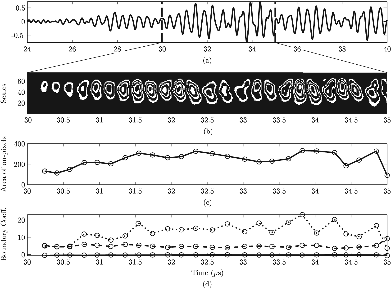
A visual summary of the DWFP (Hou and Hinders, 2002) feature extraction technique. (a) A typical ultrasonic signal and (b) a close-up portion of the DWFP output. From each “fingerprint” object, a variety of measures are extracted and interpolated in time, including (c) the area of the on-pixels for each object and (d) the coefficients of a second-order polynomial (
Another wavelet-based feature used in classification is generated by wavelet packet decomposition (Learned and Willsky, 1995). A wavelet packet transform (WPT) is applied to each low-pass filtered waveform with a specified mother wavelet and number of decomposition levels. This generates a tree of coefficients similar in nature to the wavelet transform. From the WPT tree, a vector is computed containing the percentages of energy corresponding to the terminal nodes of the tree, known as the wavelet packet energy. Because the WPT is an orthonormal transform, the entire energy of the signal is preserved in these terminal nodes (Feng and Schlindwein, 2009). Singular value decomposition is then applied to the energy matrix, returning the eigenvector with the highest energy. The corresponding elements from the WPT are used as features. In the case of multiple nodes being selected, all corresponding WPT elements are included in the feature set. Wavelet packet decomposition uses redundant basis functions and can therefore provide arbitrary time–frequency resolution details, improving upon the wavelet transform when analyzing signals containing close, high-frequency components. Wavelet packet decomposition features are included to provide insight into the generation of high-frequency modes as a result of mode conversion at flaw boundaries.
Utilizing CHomP
Before we can use the CHomP algorithms, we first need to transform our data set from several clusters of points in the feature space into a form that can be read by the computational homology algorithms. The goal is to turn these data into a cubical set, where each class is represented by a hyper-rectangle embedded in the space
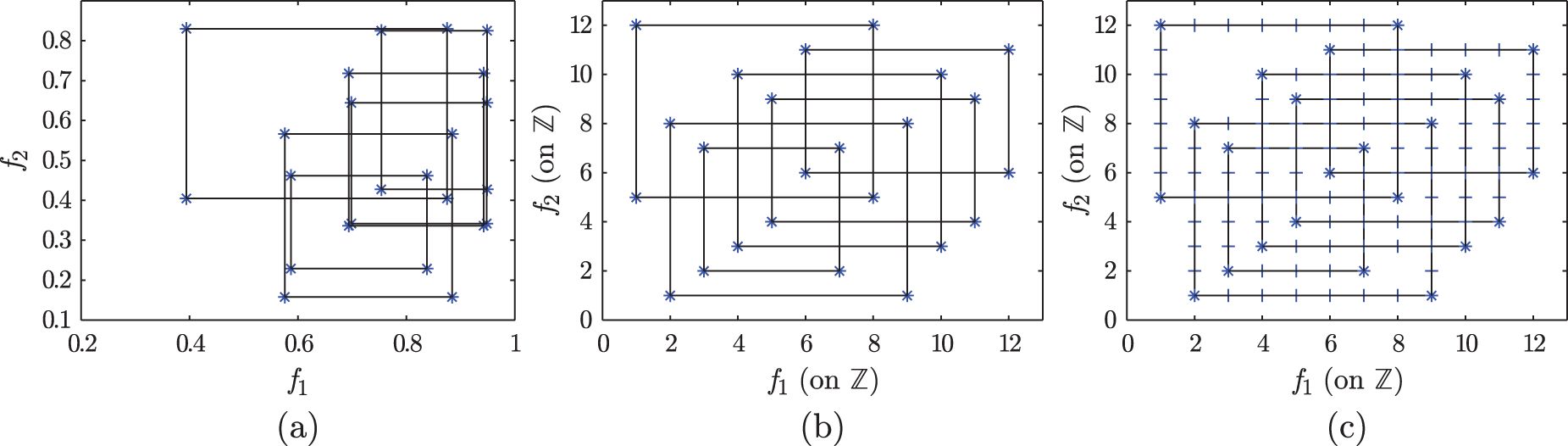
An example of converting a six-class distribution in a two-dimensional feature space into a cubical set. (a) The first step in computing the homology is to establish the class bounds in the feature space, defined here as the standard deviation in each dimension centered at the class centroid. (b) A mapping is then applied that maintains the homology of the space and sets these bounds to the integer lattice
To summarize, each d-rectangle is represented by a set of
For each feature space, the set of elementary intervals defining the hyper-rectangles in
There are computational restrictions that need to be taken into account before the CHomP algorithms are used. For the most part, the restrictions are based on the fact that each class has to be composed of elementary cubes, defined on the set of integers. It follows that a large number of classes results in a large number of elementary components required to build the resulting hyper-rectangles in the feature space. This exponentially increasing number of elementary cubes required to define a higher dimensional feature space translates to an exponential increase in the memory required to define the space. Additionally, the number of elementary cubes required in each dimension depends on number of classes present, which defines the range in each dimension for the feature space. For example, a six-class feature space will have 12 boundaries in each dimensions (an upper and lower bound per class). This further increases the memory required to define a class distribution as a cubical set. It is easy to see how the size of this problem increases drastically as the number of classes and dimensions increase.
Classifier design
We implement a supervised statistical pattern classification routine here, where new patterns are assigned class labels using the natural structure of the training data. By using a statistical approach where each pattern is represented as a point in a multidimensional feature space, we retain the physical interpretation of each feature. That is, while abstract, each feature can be connected directly back to the waveforms themselves. For example, the number of ridges in each fingerprint corresponds to waveform peak height. Since the goal of this analysis is to determine flaw severity, we assign class labels to each of the six flaw depths
There is a generally accepted phenomenon in high-dimensional spaces known as the curse of dimensionality, which identifies the concept that a finite-sized data set becomes sparse when represented in too high of a dimensional space. A rule of thumb commonly used in pattern classification is that the number of training samples per class (n) should be at least 10 times as many dimensions (d) as there are in the feature space (
We have chosen to use a quadratic discriminant classification (QDC) algorithm here because it was shown to perform best in the work performed in preliminary results (Miller and Hinders, 2013), where a more complete exploration of multiple classifier performance was considered for a similar incremental damage analysis. It was shown that the QDC results were among the best in both classifier development and validation testing.
The full six-class data set is split into training (80%) and testing (20%) subsets using random sampling (preserving class distributions) for classification. For each feature subspace under consideration, the waveforms selected as the training set are submitted to the classifier using only the features identified by the feature space. The testing subset is then submitted to the trained classifier, again using only those features defined by the feature space, and the resulting predicted labels are stored in an array. Classification accuracy is then determined to be the number of labels predicted to be within ±1 flaw depth of their actual label, presented here as a percentage of the total waveforms tested.
Results
We first present results from the computational homology analysis to identify trends present between class overlap and corresponding classification accuracy in a given feature space. The Betti numbers for all feature space subsets of dimension
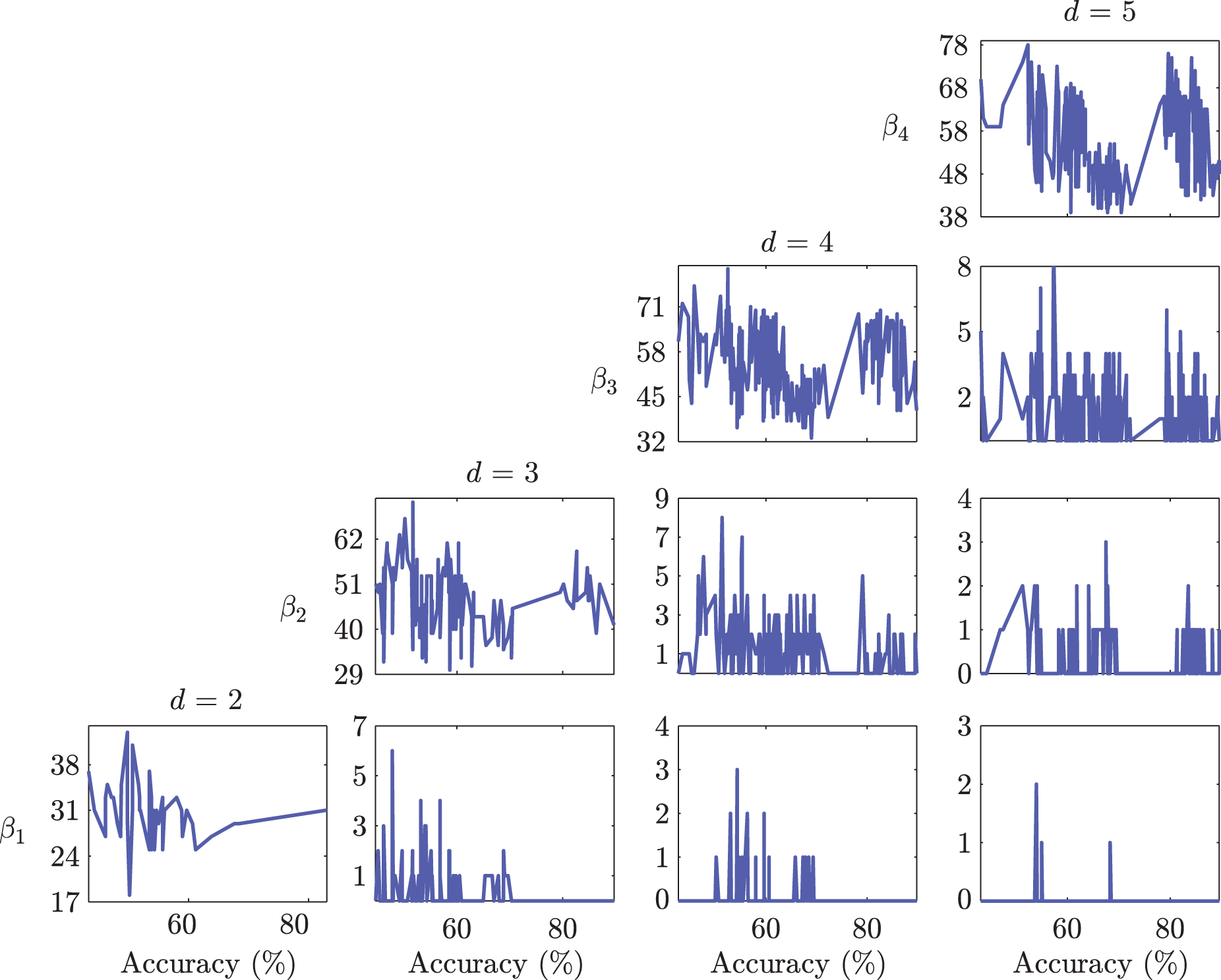
Betti number results sorted using QDC classification accuracy. Each row corresponds to Betti number
Since
For plots of
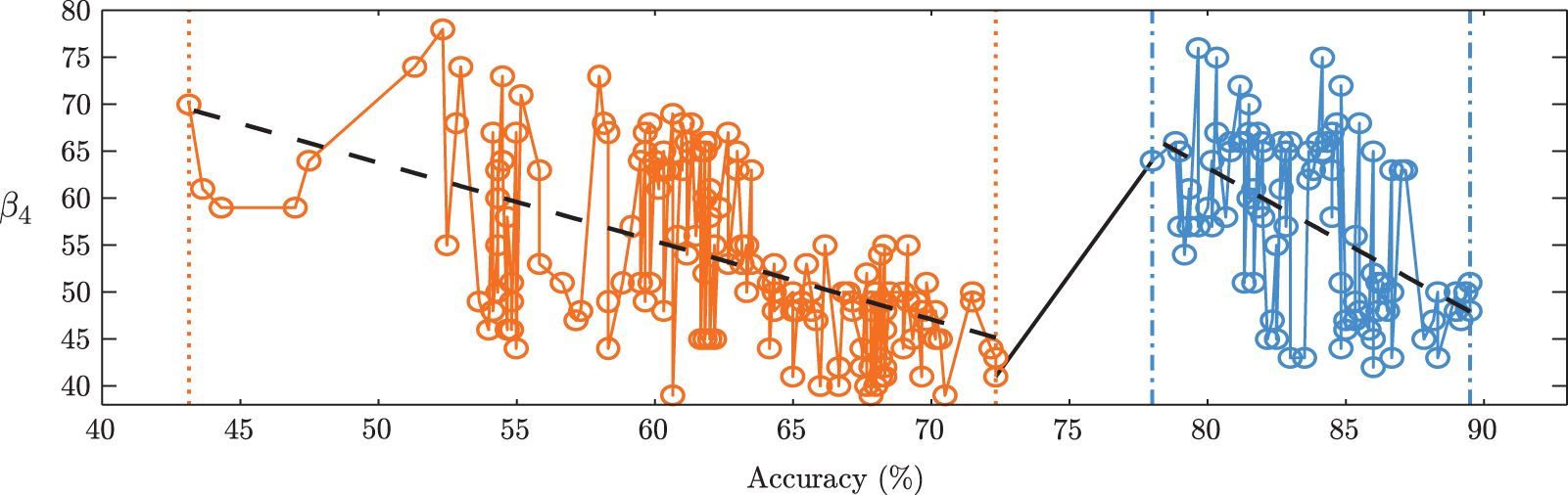
A plot of
The cause of this gap in classification accuracies is unknown, but it may be related to the concept of nested classes in the feature space being topologically identical to disjoint classes. In other words, only classes that overlap each other contribute to the increase in n-holes and therefore Betti number
We have shown that there is no reason to believe that lower Betti numbers will directly correspond to higher classification accuracy. This lack of correlation is possibly due to nested classes within the feature spaces. We therefore require an intermediate step to isolate only the higher accuracy cluster of feature spaces. Isolating this group of feature space subsets would allow us to then utilize the negative correlation between Betti number
We thus explore lower dimensional topological connectedness as well as several geometric measurements of the class distribution from within each feature space. That is, we combine a threshold on
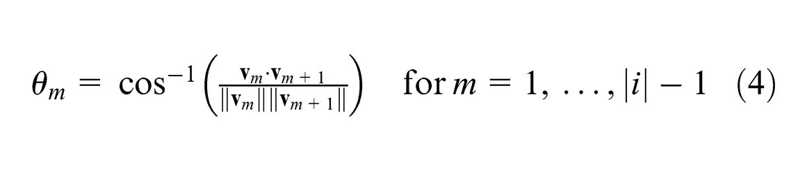
We include the maximum average distance between centroids under the assumption that classes that are spaced far apart from each other in a feature space will be easier to distinguish between, increasing classifier accuracy. We first calculate the corresponding vectors between successive n-dimensional centroids,
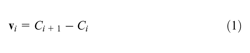
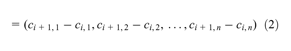
for
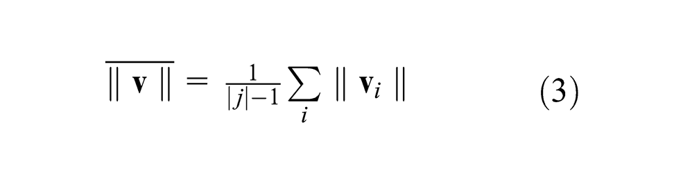
These values are sorted by highest average distance. This technique breaks down when the classes under consideration overlap significantly within the feature space due to larger intraclass spread.
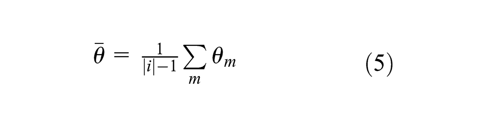
If we construct vectors between successive class centroids, we can calculate the minimum average angle between successive vectors. This measure assumes that a linear spread of classes within a feature space would result in new data of intermediate flaw severity to lie correctly between its bounding classes. For example, if data corresponding to a flaw of 35% thickness loss are introduced to a classifier, it would ideally fall somewhere in the feature space between classes
From these, we calculate the average angle between successive vectors
We sort these values by lowest average angle between class centroids in order to identify a feature space where the classes are most linearly distributed. We also calculate the tortuosity of each class centroid curve, made up of individual vectors between each successive pair of classes. Tortuosity (
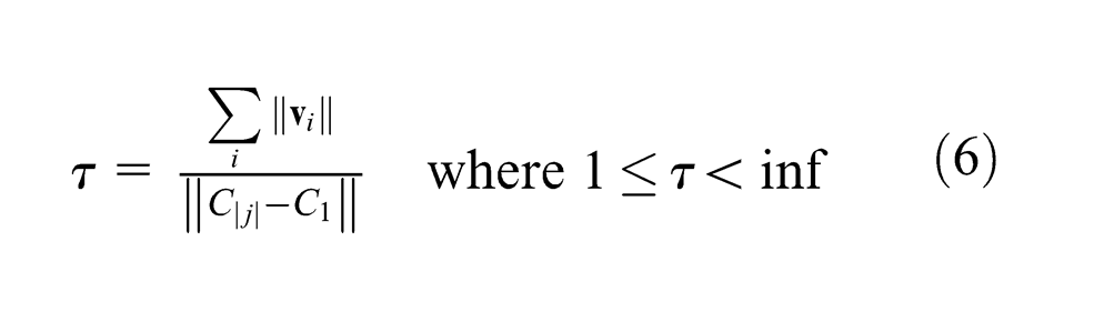
where again we have that

An example of a four-class data distribution in a two-dimensional feature space, with classes
For each feature space of dimension
For brevity, only results for
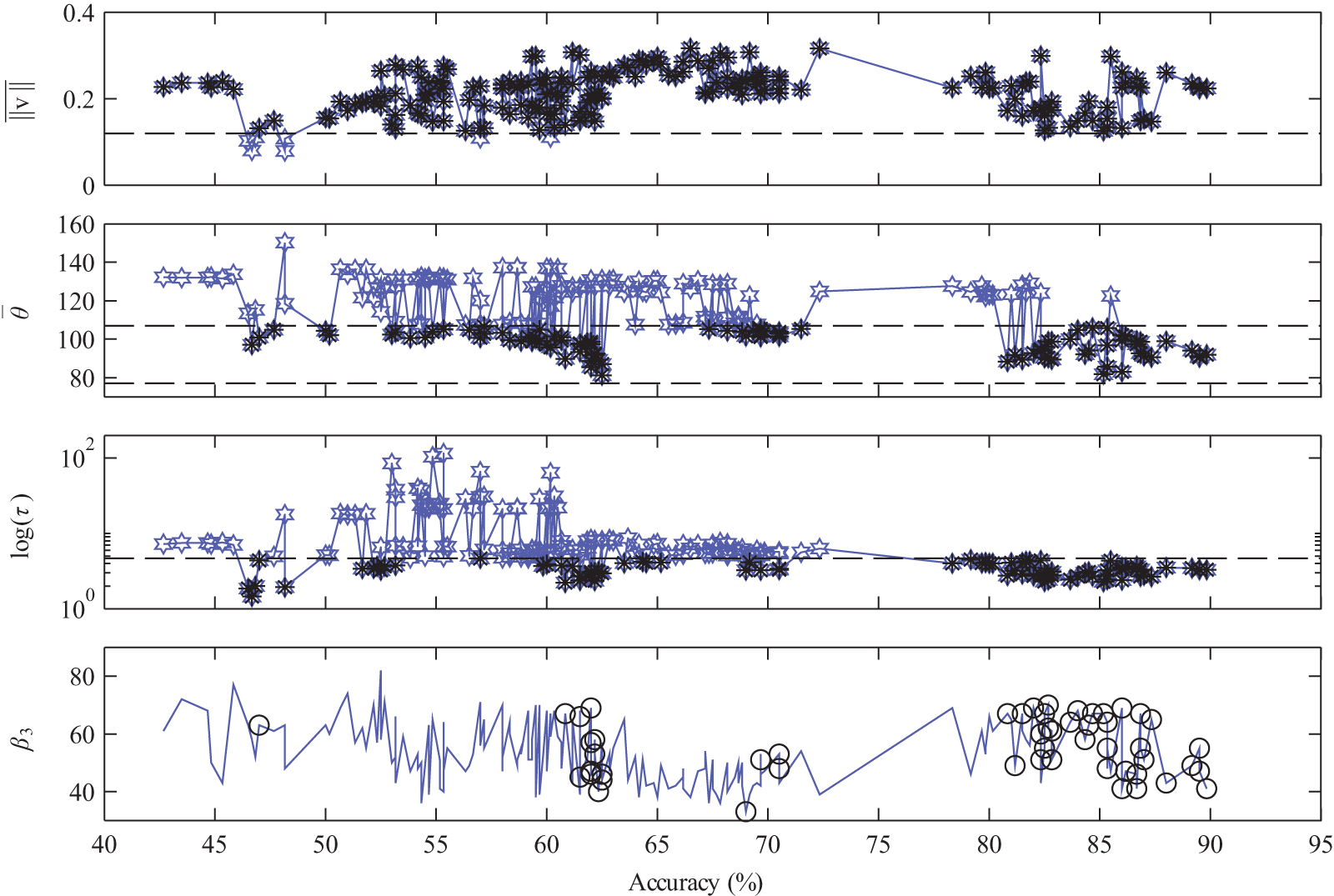
Values of the three geometric feature space versus QDC classification accuracy for all feature space subsets of dimensions
Betti numbers
Plots of
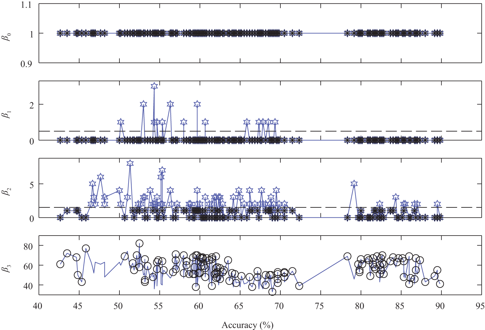
Figure 10 shows the three geometric measures plotted against their QDC accuracy, with applied thresholds represented by black dotted lines. Any data points that meet each threshold are highlighted by a black star. The bottom plot is that of
Several trends are observed in these results that are consistent across all dimensions. For the tortuosity metric, the group of feature spaces that have the highest accuracy are all clustered together below the
The average angle between centroid values also has a trend that is consistent across all dimensions. Most of the feature spaces corresponding to high classification accuracy are clustered within the
The average distance between class centroid values (
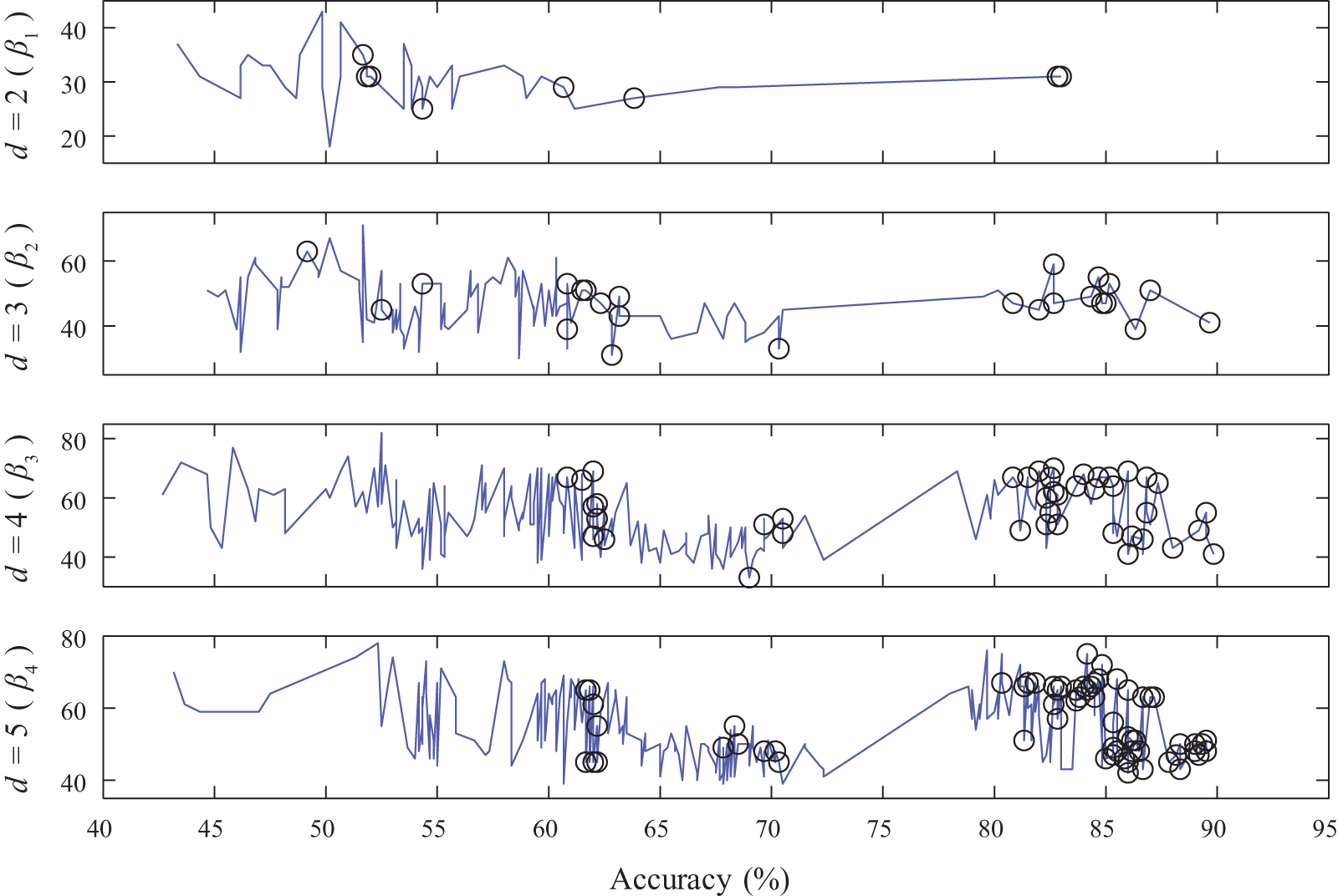
Betti number values are unique to each dimensional space as the number of nonzero
There can also exist a trade-off between how many lower accuracy feature spaces are removed and how many higher accuracy spaces are kept. It can be seen that if the threshold limit in
Feature selection results are summarized in Figure 12 for all dimensions
Conclusion
We have presented a feature selection technique using computational homology for multi-mode Lamb wave damage characterization. We first generated reconstructions of double-crosshole plate scans using LWT to identify and size the flaw at each depth. Waveforms that pass through the flaw region were automatically identified, and a subset was extracted for use with the pattern classification analysis. We generated a large number of features using a variety of signal analysis techniques, including DWFP, wavelet packet decomposition, statistical features, and Mellin domain features. We then introduced a feature selection technique that uses topological measures of the class distribution within the feature space to identify those most appropriate for Lamb wave flaw severity analysis.
We have created a filter-type feature selection routine that is able to identify subsets of a larger feature space that correlate with the highest possible classification accuracies of each subset dimension. We have approached the problem of the sequential ordering associated with a physical process that is a function of time, such as progressive damage in materials. To do this, we have measured the class overlap using a topological measure known as Betti numbers in addition to several geometric measures of the class distribution within each potential feature subspace. We have shown that applying thresholds to these measures allows for the identification of high-accuracy feature subspaces. From these remaining feature spaces, we have shown that a class distribution’s Betti numbers in feature spaces of dimension
Our work provides insight into the potential use of computational homology algorithms for studying the topological structure of class distributions within various feature spaces. For applications where the sequential ordering of classes is important, as it is in Lamb wave SHM, comparing the Betti number
Footnotes
Declaration of conflicting interests
The authors declared no potential conflicts of interest with respect to the research, authorship, and/or publication of this article.
Funding
This work was performed, in part, using computational facilities at the College of William and Mary, which were provided with the assistance of the National Science Foundation, the Virginia Port Authority, Sun Microsystems, and Virginia’s Commonwealth Technology Research Fund.