Active control of parametrically excited systems

Abstract

This article discusses active control of parametrically excited systems. Parametric resonance is observed in a wide range of applications and can lead to high levels of unwanted motion. For example, in cable-stayed bridges, the vibration of the deck excites the cables axially, inducing a periodically time-varying tension. If the frequency of deck vibration is about twice the natural frequency of the cable, a parametric resonance occurs and leads to a large-amplitude swinging motion of the cable. To tackle the consequences of parametric instability, active vibration control employing a piezoelectric actuator is proposed in this article. We consider a beam subjected to an axial harmonic load that represents a parametrically excited system with a periodically varying stiffness. Using both analytical and experimental methods, we assess the stability of the beam and propose active control aimed at relocating the transition curves and hence stabilising the system via velocity feedback and pole placement. Analytical relationship between the transition curves and the poles of the system is derived. Transition curves can be assigned to a prescribed location using appropriate velocity and displacement control gains. Finally, we demonstrate the proposed approach with experiments on a beam equipped with a macro fibre composite patch.

Keywords

Active vibration control parametrically excited systems pole placement

Introduction

Parametrically excited systems include a parameter(s) in their dynamic equations, which varies periodically in time. Parametric resonance is a dynamic instability associated with such systems. It involves interaction between the parametric excitation frequency and the natural frequency of the system, leading modes with negative damping and unstable oscillations. When the parametric excitation frequency is at about twice the natural frequency, the principal parametric resonance occurs and the system exhibits instability, leading to large oscillations and potentially fatigue or failure. One of the most common examples of this scenario is large amplitude of vibrations of cables in cable-stayed bridges. The vibration of the deck introduces a periodic variation in the tension in the cables, which under some conditions can result in parametric resonance and instability (Gonzalez-Buelga et al., 2008; Lilien and Da Costa, 1994; Reynolds and Pavic, 2006). Similar phenomena take place in flexible risers or ships, for which the wave motion can be the source of parametric excitation (Ahmed et al., 2010).

Parametrically excited systems have been the subject of research for decades (Cartmell, 1990; Nayfeh and Mook, 2008). The most simple and widely used equation of parametric excitation is the well-known Mathieu equation with linear, periodic, time-varying stiffness. This rather simple single degree-of-freedom (DOF) mechanical system exhibits complex unstable behaviour, and also interesting stability regions whose location depends on the amplitude and frequency of the time-periodic (harmonic) term. Parametrically excited systems exhibit combination resonances of summed or difference types. When subjected to an external forcing frequency, a periodically time-varying system will be resonant when the external forcing frequency equals the combination of natural frequency and parametric excitation frequency.

Time domain methods such as Floquet theory have been widely used to describe the dynamic behaviour of parametrically excited engineering systems such as helicopters (Peters, 1994), wind turbines or other bladed machines (Bir and Stol, 1999), rotating machinery (Flowers et al., 1998) and actuated microelectromechanical oscillators (Rhoads et al., 2006). Using Floquet transformation, the time-varying periodic dynamic system is transformed to a linear time-invariant system. Frequency domain techniques such as integral operator and harmonic balance have also been used to define the frequency response of parametrically excited systems (Wereley and Hall, 1990). The Fourier series expansion has been used by Allen (2009) and Han et al. (2010) to construct the frequency response function (FRF).

The control of parametrically excited systems received considerable attention; however, there is a little number of experimental results available. The most common control strategy in the literature is the cubic velocity feedback (Jun et al., 2007; Oueini and Nayfeh, 1999), since at the parametric resonance the linear damping does not reduce the amplitude of the oscillation per se (Nayfeh and Mook, 2008). However, nonlinear control involves more effects, such as bifurcation, that need to be accounted for properly. Some experimental results on a combined linear and cubic velocity feedback that include the bifurcation control have been presented in Chen (2006) and Chen et al. (2009). Lacarbonara et al. (2007) employed a perturbation analysis to design a nonlinear controller for a parametrically excited simply supported beam and demonstrated its effectiveness with the experiment. Other researchers investigated the concept of the time-varying control. Sinha and Joseph (1994) used the Lyapunov–Floquet transformation to control periodic-time-varying systems. Montagnier et al. (2001) presented a least-square equivalent controller for time-periodic systems and discussed the pitfalls of the Floquet-based approach.

Recent research emphasises the potential for introducing parametric excitation deliberately to increase system’s capability of suppressing vibration (Dohnal and Mace, 2008; Ecker, 2010). Parametric excitation can also be exploited for energy harvesting. Daqaq et al. (2009) investigated the problem of energy harvesting using a parametrically excited cantilever beam. Jia and Seshia (2013) presented a feasibility study on the use of parametrically excited bi-stable systems to increase the harvested power. The performance of parametric energy harvester was also recently investigated by Zaghari et al. (2014), who studied a piezo-equipped beam with an electromagnetic system for changing the stiffness of the harvester.

In this article, we look at the active control of a parametrically excited system from the perspective of its inherent properties and the location of the stability curves. The approach is somewhat similar to that presented in a recent article by Moreno-Ahedo et al. (2014). We adopted a vertically mounted cantilever beam subjected to a periodic axial excitation as a representative physical model for a parametrically excited system. The stability boundaries for the principle parametric resonance were investigated both analytically and experimentally. In order to tackle large-amplitude vibration at the parametric resonance, two strategies for active control of a time-periodic system, namely, velocity feedback and pole placement, are introduced. The active control proposed in the article aims at relocating stability boundaries, so that the system at given operating conditions is no longer in the unstable region. The control gains required to assign closed-loop transition curves are obtained analytically. Some aspects of the proposed approach are discussed with the aid of numerical simulations. Finally, we demonstrate the active control experimentally stabilising the parametric resonance in a beam equipped with a macro fibre composite (MFC) patch.

Stability of a parametrically excited system

System model

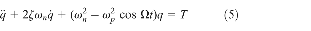
In this article, we consider a vertical cantilever steel beam subjected to an axial time-harmonic acceleration $a (t)$ as a representative physical model for a parametrically excited system. A distributed axial load resulting from the base acceleration is expected to alter the stiffness and hence the natural frequency periodically. It is assumed that the modes of the cantilever are well separated and can be treated as decoupled. Therefore, vibration of an axially loaded cantilever at its first mode can be described using a single DOF system equation with a time-varying natural frequency. We add a damping term to obtain

\overset{\cdot\cdot}{q} + 2 ζ ω_{n} \overset{\cdot}{q} + (ω_{n}^{2} - ω_{p}^{2} \cos Ω t) q = 0

(1)

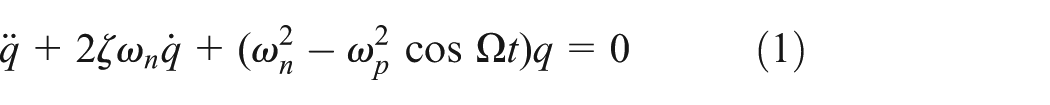
Equation (1) is in the form of the well-known damped Mathieu equation with a periodic time-varying stiffness, where $q (t)$ is the displacement response of the system, $ζ$ is the damping ratio, $ω_{n}$ is the natural frequency with no base acceleration, $ω_{p}$ is the parametric amplitude dependent on the magnitude of the base acceleration $a (t)$ and $Ω$ is the base acceleration frequency.

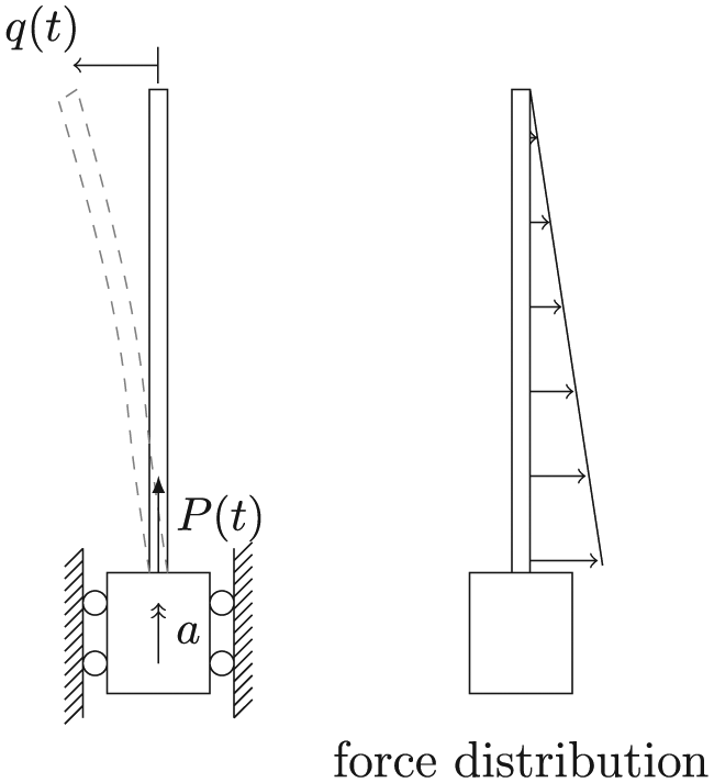
The cantilever beam considered in this article is mounted vertically on an accelerating base. Since the mass is distributed along the beam, the load is not uniform over the length of the beam (see Figure 1), which needs to be accounted for when calculating both the natural frequency $ω_{n}$ (self-weight effect) and the time-varying component of the natural frequency related to $ω_{p}$ . The relationship between the axial load and the natural frequency of a cantilever can be obtained from, for example, Shaker (1975). Modelling of parametric vibration of vertically mounted beams with accelerating bases was discussed in detail by, for example, Crespo da Silva and Glynn (1978) or Zavodney and Nayfeh (1989).

Figure 1.

A physical model of a parametrically excited system – a cantilever beam subject to a harmonic axial load.

Stability using the harmonic balance method

The response of a parametrically excited is approximated using the Fourier series

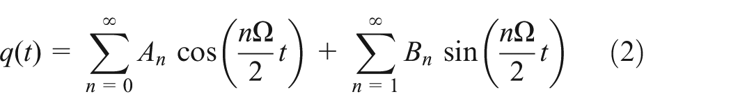
q (t) = \sum_{n = 0}^{\infty} A_{n} \cos (\frac{n Ω}{2} t) + \sum_{n = 1}^{\infty} B_{n} \sin (\frac{n Ω}{2} t)

(2)

Taking derivatives of equation (2), substituting them together with equation (2) into equation (1) and separating the $\sin (n Ω t / 2)$ and $\cos (n Ω t / 2)$ terms lead to a set of equations in terms of the coefficients $A_{n}$ and $B_{n}$ . The equations can be written in a matrix form for odd and even coefficients of $A_{n}$ and $B_{n}$ separately. As an example, the simplest case $(n = 1)$ representing the principal parametric resonance is considered. The system equation becomes

[\begin{matrix} ω_{n}^{2} - \frac{ω_{p}^{2}}{2} - \frac{Ω^{2}}{4} & ζ ω_{n} Ω \\ - ζ ω_{n} Ω & ω_{n}^{2} + \frac{ω_{p}^{2}}{2} - \frac{Ω^{2}}{4} \end{matrix}] (\begin{matrix} A_{1} \\ B_{1} \end{matrix}) = (\begin{matrix} 0 \\ 0 \end{matrix})

(3)

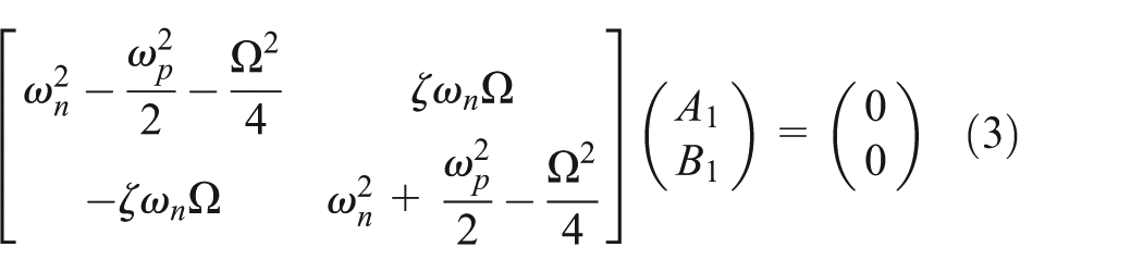
For a non-trivial solution to exist, the determinant of the above matrix must be 0, which leads to the characteristic equation

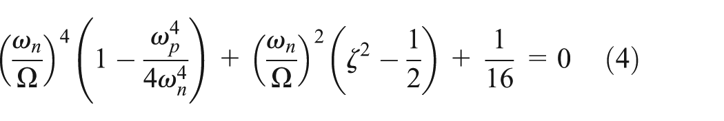
{(\frac{ω_{n}}{Ω})}^{4} (1 - \frac{ω_{p}^{4}}{4 ω_{n}^{4}}) + {(\frac{ω_{n}}{Ω})}^{2} (ζ^{2} - \frac{1}{2}) + \frac{1}{16} = 0

(4)

The roots of equation (4) constitute curves that separate the stable from the unstable regions in the parametric frequency–parametric amplitude plane. These curves are often called transition curves (or stability curves). In this article, we consider the principal parametric resonance only. Whenever the system operates within the stability tongue, its response grows without bound. Conversely, if outside the stability tongue, its response decays freely and is not affected by the parametric excitation. Finally, if the system operates at conditions exactly at the stability curve, it is marginally stable and vibrates at constant amplitude.

An illustrative example is shown for a steel cantilever beam of dimensions and properties as listed in Table 1. The natural frequency associated with the first bending mode accounting for the weight of the beam was found to be $f_{n} = ω_{n} / 2 π = 3.18 Hz$ .

Table 1.

Beam dimensions and material properties.

Property	b (m)	d (m)	L (m)	E (GPa)	$ρ$ (kg/m³)	$ζ$
Value	0.0105	0.00144	0.583	186	7850	0.001

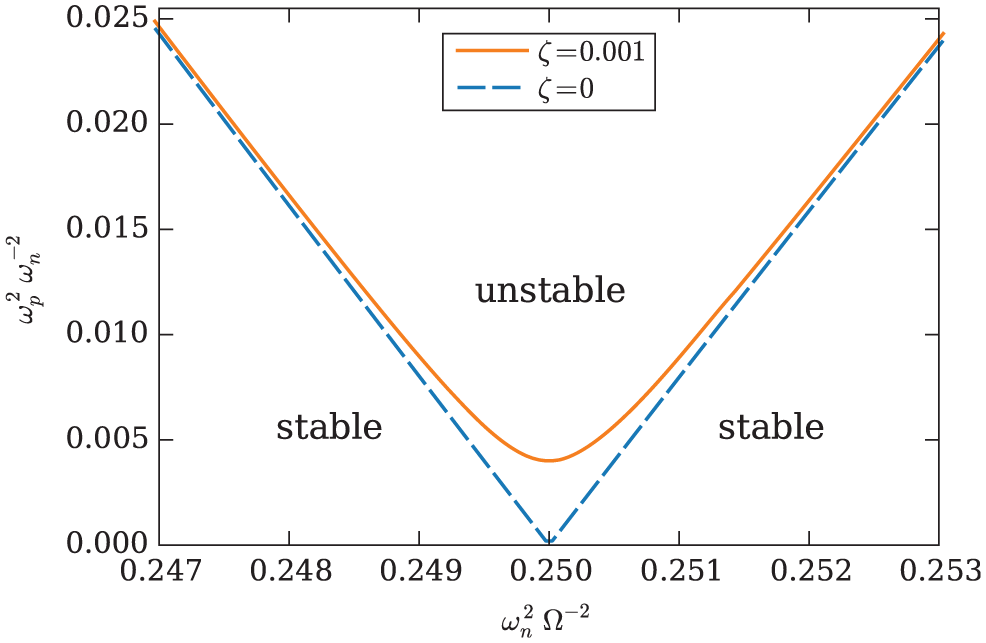
Transition curves for the principal parametric resonance are plotted using the analytical approximation in Figure 2. The two curves represent an undamped (dashed line) and a damped (solid line) system. The principal parametric instability occurs when the parametric excitation frequency is twice the first natural frequency $(Ω = 2 ω_{n})$ . The increase in damping results in an upwards shift of the transition curves, which enlarges the stable region. If higher order terms in the Fourier series are considered, transition curves associated with other parametric resonances can be obtained.

Figure 2.

Transition curves for the beam subject to an axial load – the area above the curves is unstable. The transition curves are shown with no damping and for damping ratio of 0.001.

Solving equation (4) for $Ω = 2 ω_{n}$ shows that the relationship between the parametric amplitude at which the system becomes unstable and the damping ratio is linear. It is noted that the axial load that invokes parametric instability is much lower than the static Euler buckling load. Thus, in a lightly damped system, even a small axial perturbation can make it unstable.

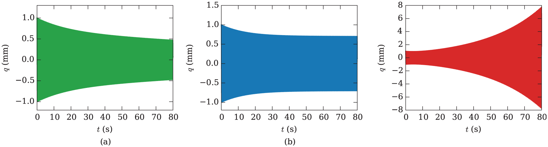
Numerical simulation using an ordinary differential equation (ODE) solver proves the analytical results valid. Time histories of the displacement response for different parametric amplitudes $ω_{p}^{2} ω_{n}^{- 2}$ and an initial displacement of $q = 1 mm$ are shown in Figure 3. The system is stable for parametric amplitudes fulfilling the condition $ω_{p}^{2} ω_{n}^{- 2} < 0.004$ , as shown in Figure 3(a), and unstable for $ω_{p}^{2} ω_{n}^{- 2} > 0.004$ (Figure 3(c)). The response of the system exhibits a limit cycle oscillation (Figure 3(b)) when excited at $ω_{p}^{2} ω_{n}^{- 2} = 0.004$ . In this case, the system is on the transition curve.

Figure 3.

Time-response of the parametrically excited beam with damping ratio 0.001 when excited at twice its natural frequency with different parametric amplitudes: (a) $ω_{p}^{2} ω_{n}^{- 2} = 0.003$ , (b) $ω_{p}^{2} ω_{n}^{- 2} = 0.004$ and (c) $ω_{p}^{2} ω_{n}^{- 2} = 0.01$ .

Experimental results

To illustrate the described phenomenon, a simple physical model was designed and constructed. A steel cantilever beam was vertically mounted on a shaker table in a way that emulates a clamped boundary condition. The shaker provided an axial excitation to the beam, which was indirectly measured by an accelerometer placed on the shaker table. Transverse vibration of the cantilever was recorded using a laser vibrometer. The experimental set-up together with the details of the equipment in place is schematically shown in Figure 4, whereas the dimensions and properties of the beam are the same as listed in Table 1.

Figure 4.

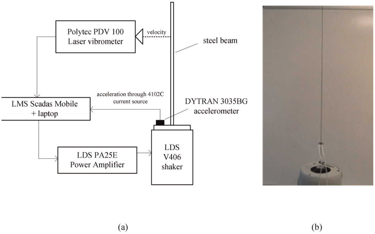
Experimental set-up for identifying the transition curves: (a) schematic diagram and (b) photograph of the beam.

First, the natural frequency associated with the first bending mode of the vertically mounted cantilever was determined via an impact hammer test. Based on this result, the parameters of the beam were identified (Table 1).

The transition curves were experimentally determined by sweeping through the excitation frequencies close to $2 ω_{n}$ at different levels of the axial load and analysing the shape of the time histories of transverse vibration. The system was qualified as stable if its response decayed exponentially with time and as unstable if the response was growing and experiencing a limit cycle oscillation. The growth of the response is limited by nonlinearities as discussed by Oueini and Nayfeh (1999).

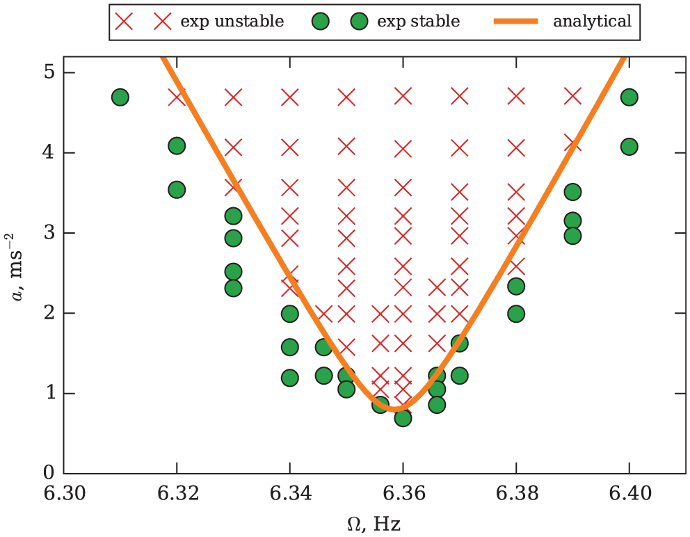
The experimental results compared to theoretical transition curves derived in the previous section are presented in Figure 5. The direct relationship between the non-dimensional parametric amplitude $ω_{p}^{2} ω_{n}^{- 2}$ and the base acceleration may be found with the aid of any of the models available in the literature (see e.g. Crespo da Silva and Glynn, 1978; Zavodney and Nayfeh, 1989 for reference). In this article, we focus on the active control of the parametric resonance; hence, we adopted a scaling constant that makes the dip of the experimental and the analytical transition curves match.

Figure 5.

Transition curves – comparison between the experiment and the analytical prediction.

The experimental results are in very good agreement with the theoretical predictions. In Figure 6, we present chosen velocity time histories and their Fourier transforms for the stable and the unstable case. The influence of additional nonlinearities in the experimental set-up is evident in the response at the unstable state. The amplitude initially increases as a consequence of parametric excitation but at some level becomes limited by the nonlinearities.

Figure 6.

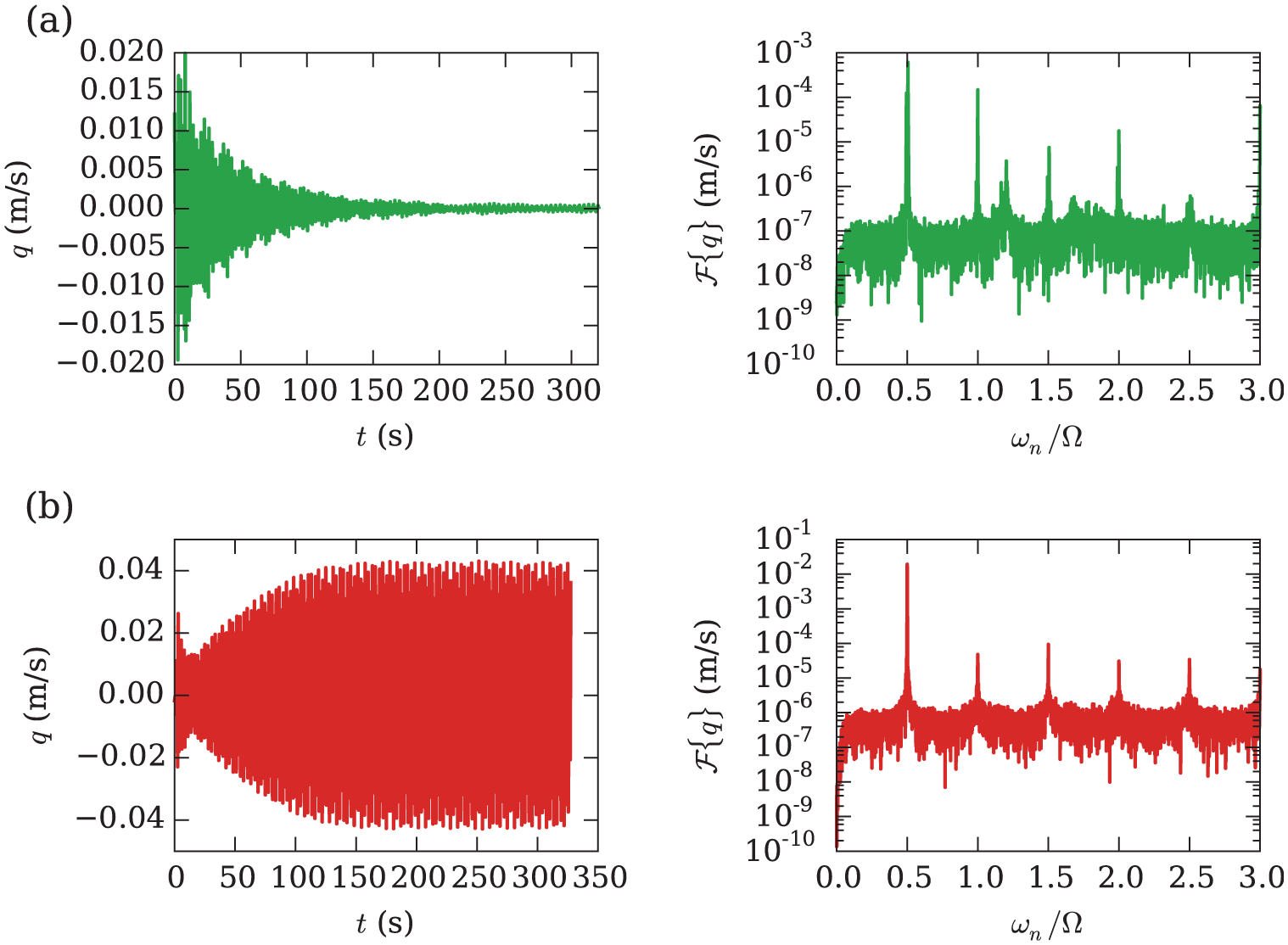
Measured response time histories and their Fourier transforms: (a) stable and (b) unstable.

Active vibration control of a parametrically excited system

The most common approach to active control of the parametric resonance is to employ constant cubic velocity feedback or constant combined cubic and linear velocity feedback. The choice of the cubic control law is supported by the fact that the amplitude of vibration of a parametrically unstable system cannot be reduced by viscous-type damping. On the contrary, introducing nonlinear damping provides the way to limit the vibration, since the presence of the nonlinearity results in a steady-state limit cycle oscillation at an unstable condition. In fact, cubic velocity feedback is not capable of cancelling vibrations associated with parametric resonance entirely on its own. The response of the closed-loop system is suppressed only if the model of the system includes several other nonlinear effects, as done by, for example, Oueini and Nayfeh (1999) or Chen (2006).

In this article, we propose an alternative time-invariant feedback control which aims at altering the characteristics of the time-varying system. Both damping and stiffness of the structure influence the location and the shape of the transition curves and hence the instability region. The main concept of the control proposed in this article is to alter the characteristics of the system which results in shifting the unstable region and transition curves away from the operating point. If the system is initially unstable, active control stabilises the vibration. If the system is initially stable but close to a transition curve, active control moves that transition curve further away from the operating point so that the system is less prone to becoming parametrically unstable.

The approach is different from a methodological perspective – the control is supposed to relocate the transition curves in order to make the system stable under specified conditions. In other words, we address the source of high-amplitude vibration directly. Although simplistic in nature, the technique is shown to be effective and easy to implement.

In the following sections, we compare different control laws by investigating the effect of the feedback control on both the transition curves (steady-state) and the transient response of the system. The control law is introduced to the system equation as follows

\overset{\cdot\cdot}{q} + 2 ζ ω_{n} \overset{\cdot}{q} + (ω_{n}^{2} - ω_{p}^{2} \cos Ω t) q = T

(5)

where $T$ is the control law.

Velocity feedback

Velocity feedback is considered first. The control law takes the form

T = - h \overset{\cdot}{q} (t)

(6)

where $h$ is the velocity feedback gain. We substitute equation (6) into equation (5) and use the first-term Fourier expansion from equation (2). Grouping respective harmonic components, we obtain the following non-trivial solution condition (detailed manipulation is omitted here for the sake of brevity)

{(\frac{ω_{n}}{Ω})}^{4} [1 - \frac{ω_{p}^{4}}{4 ω_{n}^{4}}] + {(\frac{ω_{n}}{Ω})}^{2} [{(ζ + \frac{h}{2 ω_{n}})}^{2} - \frac{1}{2}] + \frac{1}{16} = 0

(7)

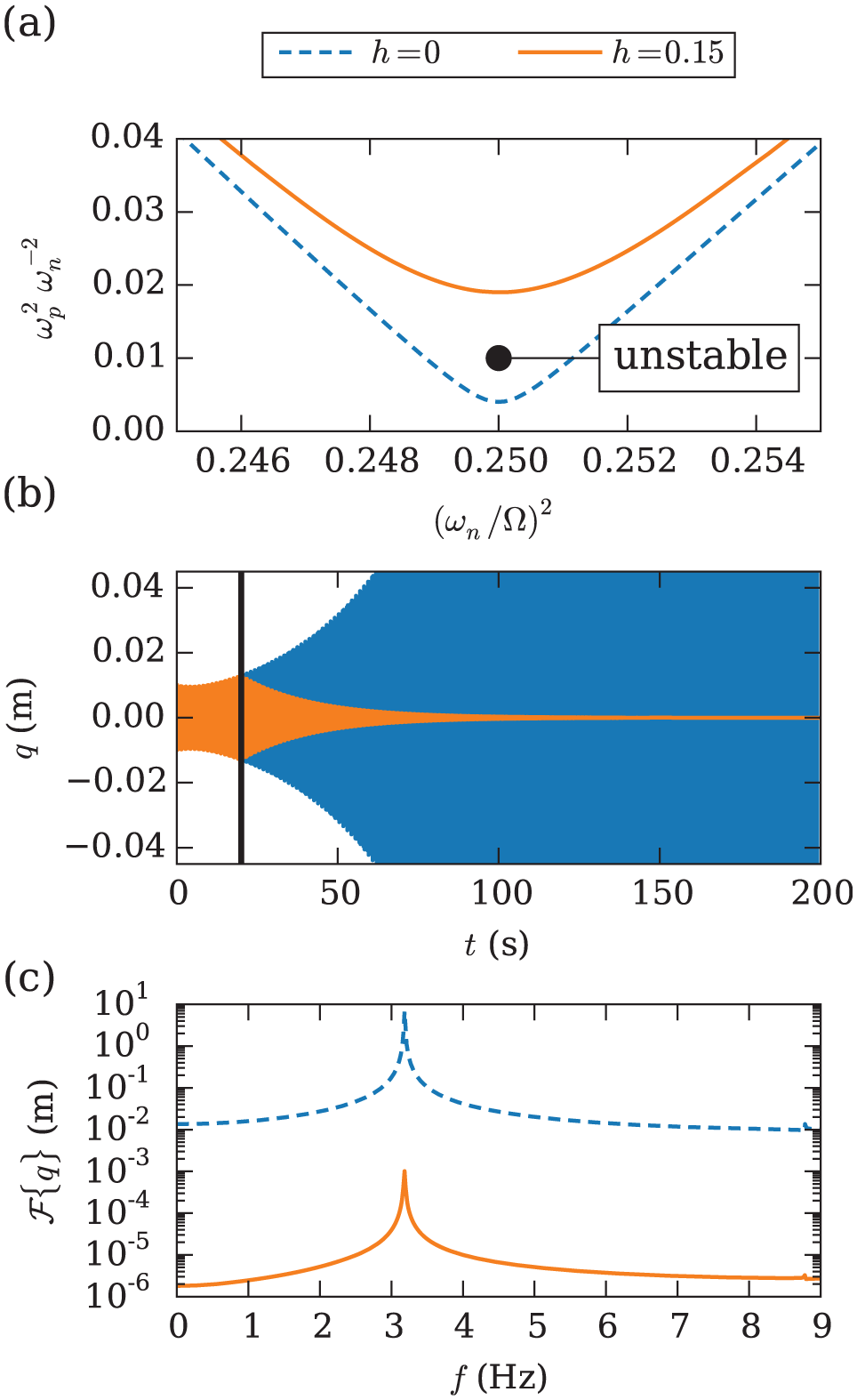
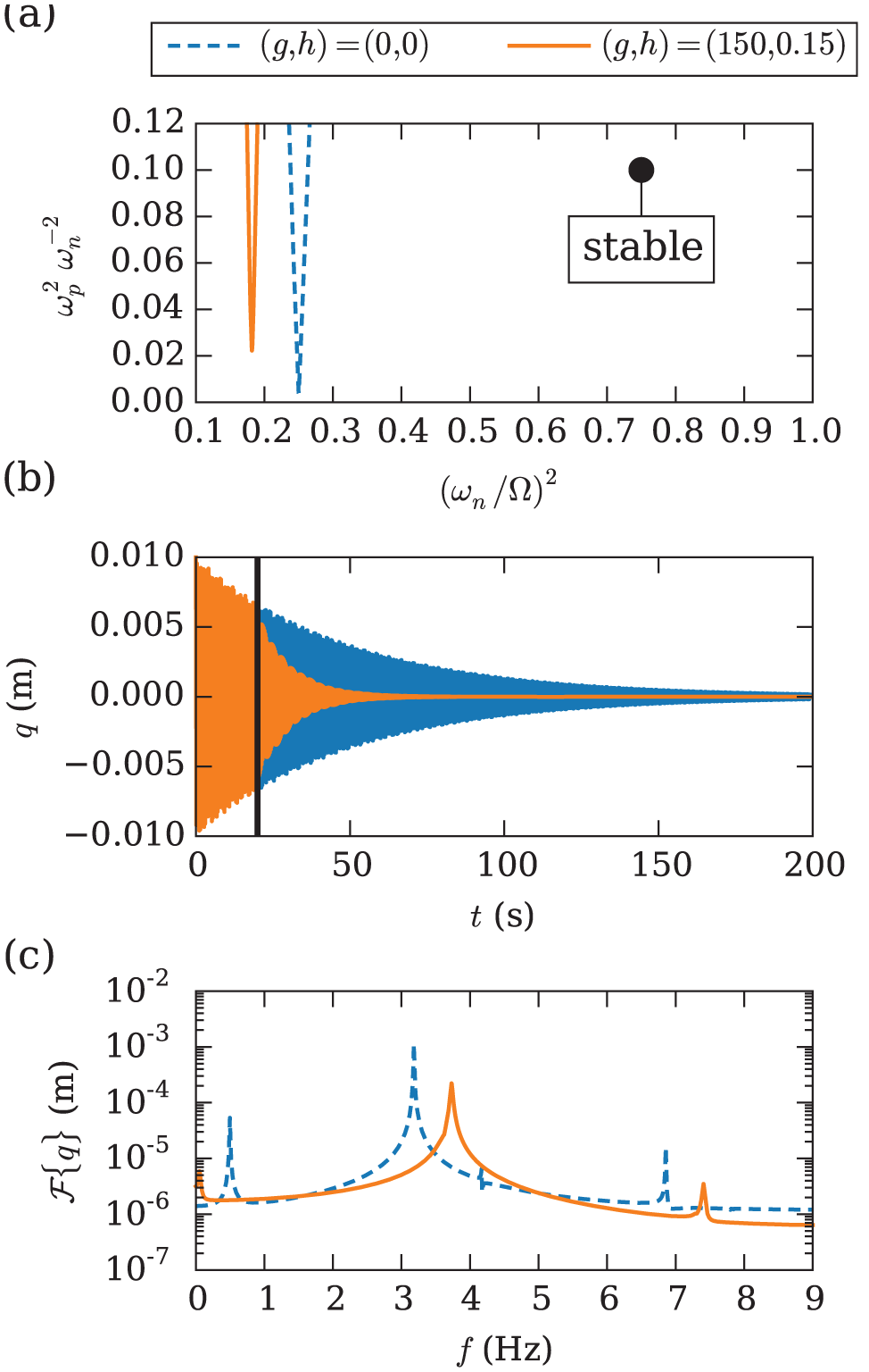
We investigate the effect of the control force using an illustrative example in which the closed-loop velocity feedback gain is chosen to be $h = 0.1$ . The transition curves are calculated using equation (7), whereas the time histories corresponding to a chosen configuration are obtained numerically from an ODE solver. We consider two open-loop configurations, namely, an initially unstable and an initially stable system. The unstable condition is achieved for parametric excitation amplitude $ω_{p}^{2} ω_{n}^{- 2} = 0.01$ and frequency such that $(ω_{n} / Ω)^{2} = 0.25$ . The stable condition refers to $ω_{p}^{2} ω_{n}^{- 2} = 0.1$ and $(ω_{n} / Ω)^{2} = 0.75$ . The simulation results for both cases are shown in Figures 7 and 8, respectively.

Figure 7.

Effect of velocity feedback on an initially unstable parametrically excited system: (a) transition curves, (b) time histories from numerical simulation – the vertical line indicates when active control was activated and (c) FFT of the time histories.

Figure 8.

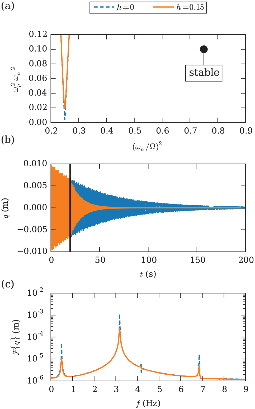
Effect of velocity feedback on an initially stable parametrically excited system: (a) transition curves, (b) time histories from numerical simulation – the vertical line indicates when active control was activated and (c) FFT of the time histories.

Let us first look at the initially unstable system. The response of the open-loop system grows without bound and its energy is infinite. The system is stabilised using the chosen velocity feedback gain as shown with the solid line in Figure 7(b). It becomes stable because increased damping moves the transition curves upwards so that the operating conditions no longer fall into the unstable region as shown in Figure 7(a). The frequency response in Figure 7(c) is obtained by applying the fast Fourier transform (FFT) to a finite-length time window, and therefore even the peak corresponding to the parametric resonance of the unstable system has a finite amplitude. The magnitude of the response spectrum, including the parametric resonance peak, is significantly reduced as a consequence of velocity feedback control.

For the initially stable system, the effect of velocity feedback is apparent in the time response. The response decays more rapidly as a consequence of enhanced damping as shown in Figure 8(b). In Figure 8(c), we clearly observe periodic poles at $| ω \pm n Ω |$ (where $n$ is an integer) typical for a time-periodic system. The influence of the periodic poles depends on damping and on how strongly time-periodic the system is, so they are not always clearly visible in the response. Note that increasing damping reduces both the amplitude of the fundamental mode and the periodic mode. The system is less likely to become unstable if its operating conditions are slightly changed, as the velocity feedback moves the unstable region further away from the operating point.

Combined velocity and displacement feedback

Using both aforementioned feedback laws together provides more flexibility in relocating transition curves. The control law takes the form

T = - gq (t) - h \overset{\cdot}{q} (t)

(8)

where $g$ and $h$ are the displacement and velocity feedback gains, respectively. As done in the previous section, we substitute equation (8) into equation (5) and use the first-term Fourier expansion from equation (2) to determine the non-trivial solution condition

\begin{matrix} {(\frac{ω_{n}}{Ω})}^{4} [{(1 + \frac{g}{ω_{n}^{2}})}^{2} - \frac{ω_{p}^{4}}{4 ω_{n}^{4}}] \\ + {(\frac{ω_{n}}{Ω})}^{2} [{(ζ + \frac{h}{2 ω_{n}})}^{2} - \frac{1}{2} - \frac{g}{2 ω_{n}^{2}}] + \frac{1}{16} = 0 \end{matrix}

(9)

For the illustrative example, parametric excitation conditions are the same as in previous sections and feedback gains are $g = 150$ and $h = 0.15$ .

We discuss the unstable case first for which the results in both time and frequency domain are shown in Figure 9. Combined feedback control successfully stabilises the system. Transition curves are relocated so that the system no longer operates in the unstable condition – see Figure 9(a). As a consequence, the system response decays freely after the control is activated (Figure 9(b)). The frequency responses shown in Figure 9(c) confirm that the peak associated with the main mode is both reduced in magnitude and shifted towards higher frequencies.

Figure 9.

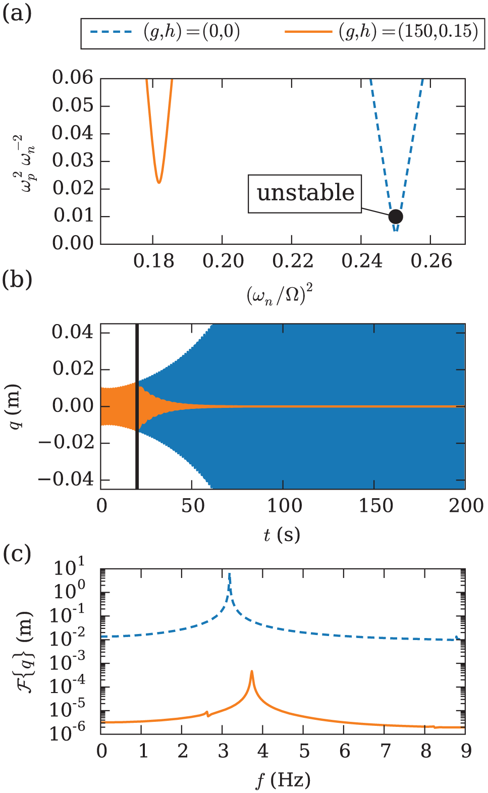
Effect of a combined velocity and displacement feedback on an initially unstable parametrically excited system: (a) transition curves, (b) time histories from numerical simulation – the vertical line indicates when active control was activated and (c) FFT of the time histories.

The results for the initially stable system are shown in Figure 10. Combined feedback moves the transition boundary further away from the operating conditions as seen in Figure 10(a). Enhanced damping makes the response in Figure 10(b) decay faster than the open-loop stable case. Finally, both the main and periodic poles of the system are relocated in an expected manner as shown in Figure 10(c).

Figure 10.

Effect of a combined velocity and displacement feedback on an initially stable parametrically excited system: (a) transition curves, (b) time histories from numerical simulation – the vertical line indicates when active control was activated and (c) FFT of the time histories.

Pole placement and transition curves relocation

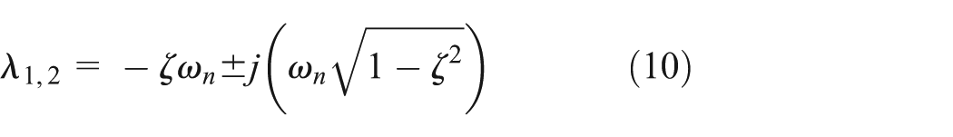
In the previous sections, we showed how active control relocates the transition curves of a parametrically excited system. The design of such active control might involve prescribing a desired transition boundary by appropriate calculation of control gains, which is directly linked to conventional pole placement. We note the fundamental pair of poles of a parametrically excited system to be

λ_{1, 2} = - ζ ω_{n} \pm j (ω_{n} \sqrt{1 - ζ^{2}})

(10)

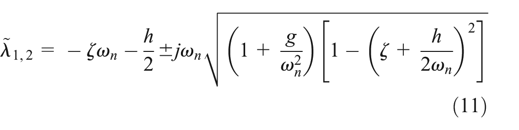
Combined velocity and displacement feedback alters the poles in the following manner

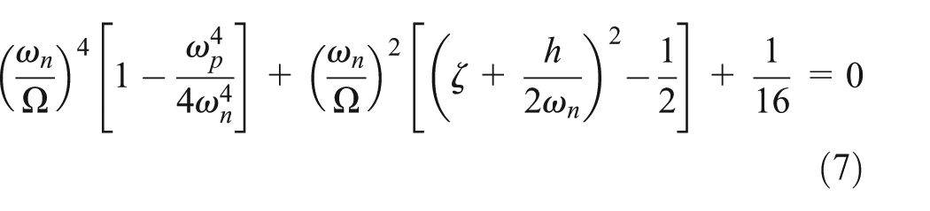
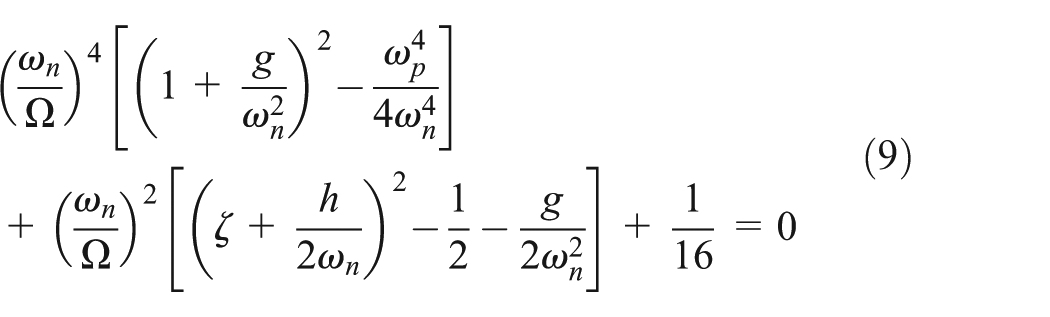
{\tilde{λ}}_{1, 2} = - ζ ω_{n} - \frac{h}{2} \pm j ω_{n} \sqrt{(1 + \frac{g}{ω_{n}^{2}}) [1 - {(ζ + \frac{h}{2 ω_{n}})}^{2}]}

(11)

Likewise, we can rearrange the characteristic equation for parametric instability with feedback control to obtain a biquadratic equation for the transition curves as a function of the frequency ratio

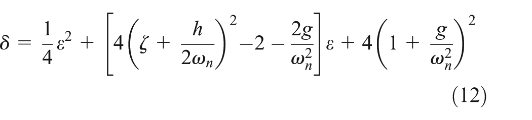
δ = \frac{1}{4} ε^{2} + [4 {(ζ + \frac{h}{2 ω_{n}})}^{2} - 2 - \frac{2 g}{ω_{n}^{2}}] ε + 4 {(1 + \frac{g}{ω_{n}^{2}})}^{2}

(12)

where $δ = ω_{p}^{4} / ω_{n}^{4}$ and $ε = Ω^{2} / ω_{n}^{2}$ . Equation (12) is a quadratic equation in $ε$ ; hence, the topographic features of the associated parabola can readily be analysed. Using equation (12), we can illustrate the link between pole placement and assignment of the transition curves.

The location of the dip of the stability tongue is of particular interest for controlling parametric resonance. From equation (12), we can write its coordinates in terms of the control gains

ε_{dip} = 4 + \frac{4 g}{ω_{n}^{2}} - 8 {(ζ + \frac{h}{2 ω_{n}})}^{2}

(13)

δ_{dip} = - {[4 {(ζ + \frac{h}{2 ω_{n}})}^{2} - 2 - \frac{2 g}{ω_{n}^{2}}]}^{2} + 4 {(1 + \frac{g}{ω_{n}^{2}})}^{2}

(14)

Equations (13) and (14) allow us to determine control gains that shift the dip of the instability tongue to a prescribed location $(\tilde{ε}, \tilde{δ})$ . The location of the dip along the frequency axis depends predominantly on the displacement feedback gain $g$ . Thus, neglecting the influence of the damping-related term enables a straightforward calculation of displacement feedback gain required to achieve certain frequency ratio $\tilde{ε}$ using equation (13). If $g$ is known, velocity feedback gain that shifts the transition curves dip vertically to $\tilde{δ}$ can be obtained from equation (14).

In principle, given a particular set of parameters on the parametric plane, one can design control to move the transition boundary precisely to that configuration with minimal power consumption in the chosen actuator. This would depend on the type of the actuator and need to be solved as a constrained with the chosen optimisation problem.

Experiments

Experimental set-up

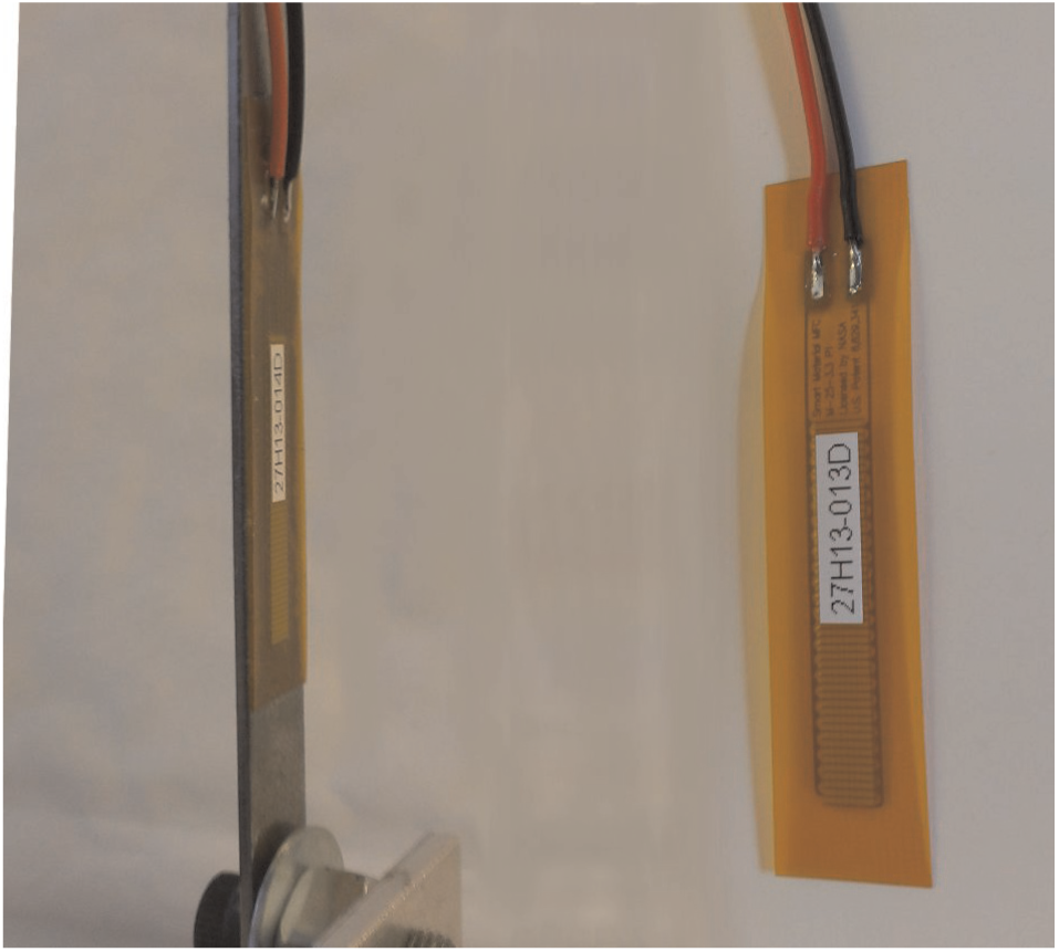
Active control was demonstrated on the physical model of a vertically mounted cantilever. The beam was equipped with an MFC patch (M2503-P1; Smart Material Corp.) with an active area of $25 \times 3 mm$ and thickness 0.3 mm bonded near the clamped as shown in Figure 11.

Figure 11.

MFC2503-P1 patch bonded to the beam.

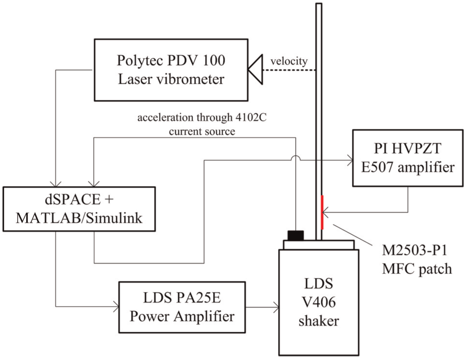
Active control was implemented digitally using a dSPACE 1103 controller coupled with MATLAB/Simulink. A schematic overview of the experimental set-up is presented in Figure 12. A simple controller was designed in Simulink and uploaded to dSPACE 1103 enabling real-time control and adjustment of parameters via dedicated dSPACE ControlDesk software.

Figure 12.

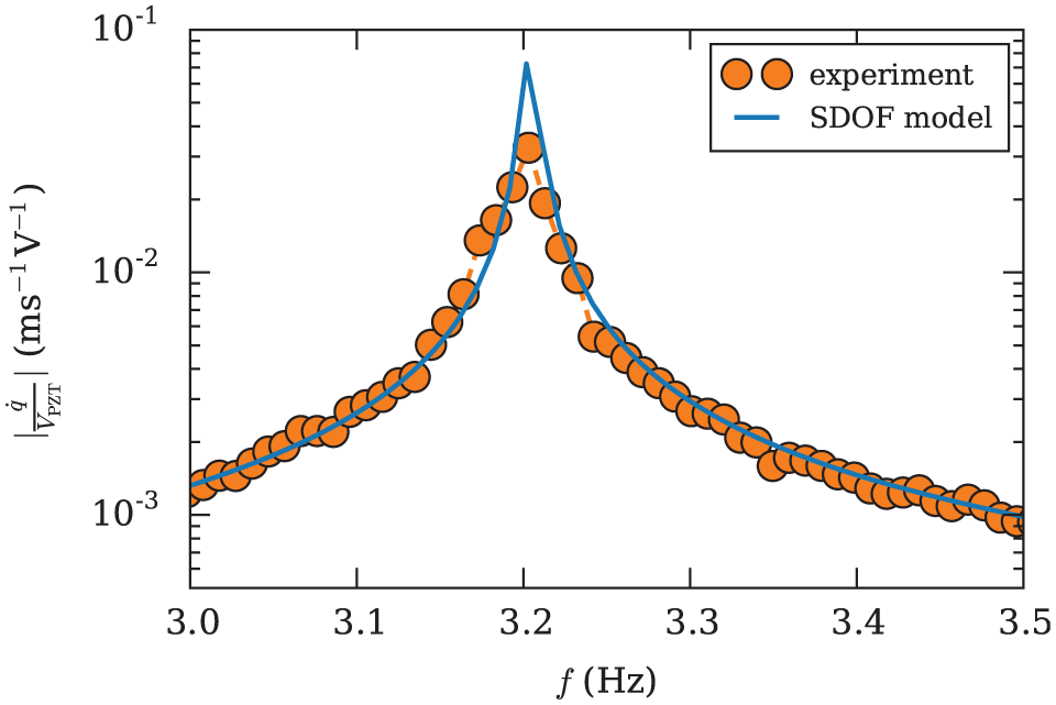
Mobility of the beam excited with the MFC patch; comparison between the experiment and the SDOF model.

Transverse velocity of the beam was measured directly using a laser vibrometer and fed into the controller unit. After appropriate band-pass filtering, velocity feedback gain could be applied to the signal. To enable implementation of displacement feedback, the velocity signal was integrated and the outcome filtered with a high-pass filter (cut-off frequency: 1 Hz) to remove the integration constant. After corresponding feedback gains were applied, the two control signals were added and sent to the amplifier.

The PI HVPZT E507 amplifier used in the experiment has a constant gain of −100 V/V, so appropriate lower and upper limits on the output signal were imposed with a saturation block in order to ensure that the voltage applied to the MFC does not exceed the allowable values.

The equation of motion for a cantilever beam excited with surface-bonded MFC patch at its first mode can be obtained using, for example, Galerkin method (Yousef and Mohammed, 2010). In this work, the governing equation was found from updating the SDOF model based on the experimental data. The forcing term associated with the MFC patch is added to the right-hand side of equation (1). The coefficient representing the excitation generated by the MFC patch was identified experimentally, so that the equation becomes

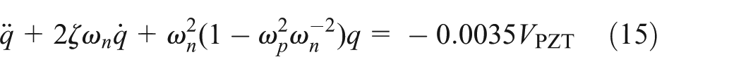
\overset{\cdot\cdot}{q} + 2 ζ ω_{n} \overset{\cdot}{q} + ω_{n}^{2} (1 - ω_{p}^{2} ω_{n}^{- 2}) q = - 0.0035 V_{PZT}

(15)

where $V_{PZT}$ is the driving voltage.

In Figure 13, we plot the mobility obtained from equation (15) and that obtained from the measurement; they are in very good agreement.

Figure 13.

Active control of a parametrically excited beam – schematic diagram of the experimental set-up.

The patch increased the stiffness of the beam, and therefore, the transition curves shifted slightly towards higher frequencies. The natural frequency of the vertically mounted cantilever with the MFC patch was found to be at 3.197 Hz. To verify how bonding of patch affected the transition curves, they were measured again using the same procedure as for the unequipped beam. The results are shown in Figure 14. Interestingly, the left arm of the transition curve diverges from the trajectory predicted by the analytical model. This is attributed to nonlinearities, influence of which became more prominent after placing the patch. Additional measurement of frequency–response curves at different levels of excitation indicates the contribution of softening cubic stiffness. As the amplitude of steady-state parametric vibration increases towards lower excitation frequencies, the effect of the cubic stiffness on the transition curves is expected to manifest itself more in the neighbourhood of the left arm of the transition curve in Figure 14.

Figure 14.

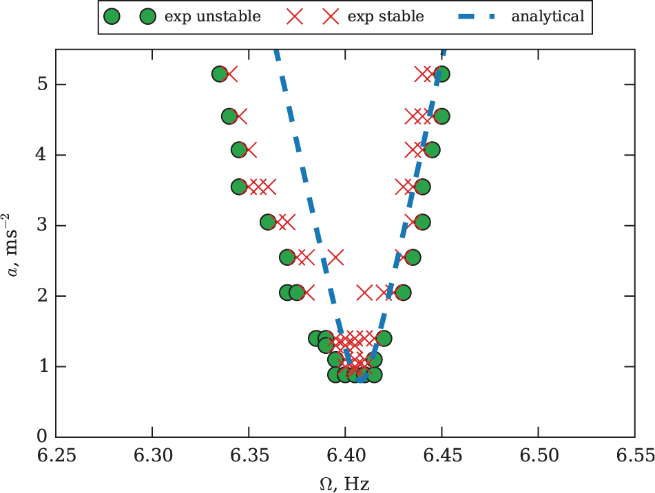
Measured transition curves for the beam with the MFC patch bonded.

Closed-loop transition curves

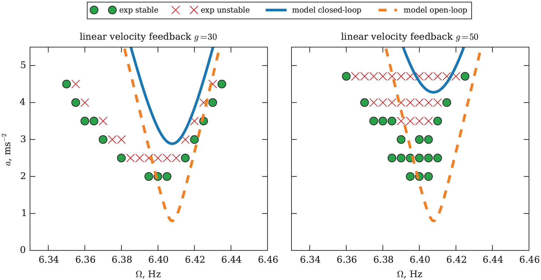
Transition curves around the principal parametric resonance were measured again using the same procedure as before for a closed-loop system with velocity feedback. Active control was switched on during the whole test with appropriate fixed gain setting. The results for two values of $g$ are shown in Figure 15. Closed-loop transition curves are squeezed upwards, as expected from the theory and the increase in $g$ results in shifting the transition curve dip even further up the amplitude axis. The trend expected from the analytical model is confirmed in the experiment; however, it is clear that the two curves do not match well.

Figure 15.

Closed-loop transition curves with velocity feedback activated: measurement and the analytical model.

The location of the dip of the transition curve along the amplitude axis predicted by the model strongly depends on the correct identification of the constant representing the coupling between the MFC patch and beam vibration. The constant identified in this article may not be accurate enough and additional measurement could refine it. We note that although the proposed approach to active control enables assigning transition curves to a prescribed location, it relies on the accurate model of the system and the coupling between the actuator and the system. In some cases, it might be considered as a disadvantage.

Moreover, it is worth noting that the analytical transition curves plotted in Figure 15 are located slightly higher along the frequency axis than indicated by the measured results. We believe that this is related to a change in the natural frequency of the beam due to the variation in environmental conditions. In this particular case, the change in the natural frequency is less than 0.005 Hz. This raises another important aspect of active control of parametrically excited systems. Variability in the natural frequency due to various external conditions, although negligible from the modal analysis viewpoint, has a significant effect on the stability curves. Parametric resonance is a narrowband phenomenon especially at low levels of parametric amplitude; thus, the variability of the natural frequency poses an additional challenge for active control design.

In the next section, we demonstrate the effect of active control in the time domain for two control strategies, namely, velocity and combined velocity and displacement feedback. The open-loop and closed-loop transition curves for both control strategies together with control gains used in the experiment are shown in Figure 16 (for the natural frequency of the system taken as 3.199 Hz).

Figure 16.

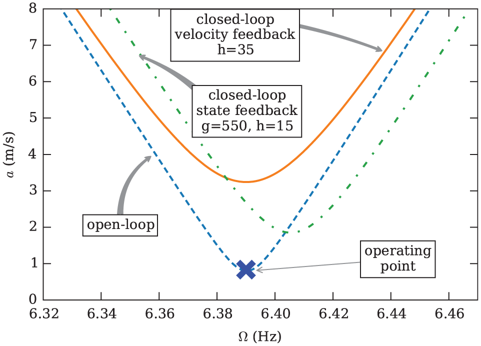
Illustration of the adopted control strategies for the experimental demonstration.

Closed-loop time response – velocity feedback

Velocity feedback increases damping in the system and shifts the transition curves up, enlarging the stable region. Although increased damping does not limit the amplitude of oscillations if the system is unstable, it alters the characteristics of the system which can be exploited for ensuring that the operating point is in the stable region.

Active control in time domain was demonstrated for the following conditions: harmonic acceleration of the base with the amplitude $a = 0.8352 {m / s}^{2}$ at 6.39 Hz. The time history of the transverse velocity of the beam is presented in Figure 17. At first, the parametric excitation pumps the energy into the system, which results in an unstable growth of the response. The steady-state limit cycle oscillations are reached as an effect of the nonlinearities in the experimental arrangement. When the feedback control is activated and the response starts to decay freely. The experimental results confirm the strategy of the control outlined in Figure 17 and indicate that the velocity feedback can stabilise the parametrically excited systems. When the velocity feedback was used ( $h = 0.1225$ ), the increased damping shifted the transition curves up so that the system at given operating conditions became stable and the parametric excitation was not able to feed energy into the system. As a consequence, the response of the system with active control has the form of free damped vibration.

Figure 17.

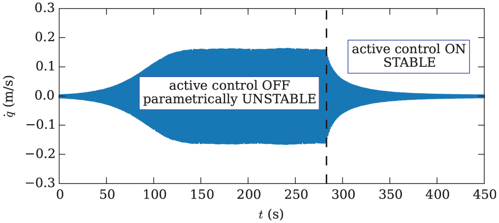
Active control of a parametrically excited beam – time history of the response demonstrating the effect of the velocity feedback.

Closed-loop time response – combined velocity and displacement feedback

Displacement feedback affects the natural frequency of the system, and therefore shifts the transition curves horizontal, whereas velocity feedback enhances damping and is capable of moving the transition curves vertically.

The corresponding time history for the considered active control strategy is shown in Figure 18. Similarly to the above, initially the beam’s response grows as the parametric excitation pumps the energy to the system. Steady-state oscillations are established when no more energy can be fed into the system due to nonlinear effects and the dissipative components. When the control is activated, the response starts to decay freely. 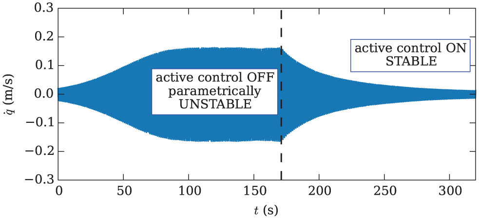The feedback gains applied ( $h = 0.0525$ , $g = 1.925$ ) caused the transition curves to shift up and to the right, so that the system under given operating conditions became stable.

Figure 18.

Active control of a parametrically excited beam – time history of the response demonstrating the effect of combined velocity and displacement feedback.

The presented demonstration of the active control showed that both the linear velocity feedback and combined velocity and displacement feedback are capable of stabilising the parametrically excited system.

Conclusion

In this article, we discussed active control of parametrically excited systems by relocating the transition curves with both linear velocity feedback and pole placement. An axially excited vertical cantilever beam served as a physical model. The stability of the beam around its principal parametric resonance was analysed both analytically, using the harmonic balance method, and experimentally. We outlined various aspects of the proposed active control showing how it affects the transition curves and the time response of both an initially stable and an initially unstable system. The effectiveness of these strategies was confirmed by numerical analyses and successfully demonstrated in an experiment on the beam equipped with an MFC patch.

Footnotes

Acknowledgements

The authors would like to thank Professor Stephen Elliott for his comments.

Declaration of Conflicting Interests

The authors declared no potential conflicts of interest with respect to the research, authorship and/or publication of this article.

Funding

The author(s) disclosed receipt of the following financial support for the research, authorship, and/or publication of this article: M. G. T. gratefully acknowledges the support provided by EPSRC for her first Grant (ref: EP/K005456/1). The authors acknowledge EPSRC programme grant on Engineering Nonlinearity (ref: EP/K003836/1).

References

Ahmed

Hudson

Temarel

(2010) An investigation into parametric roll resonance in regular waves using a partly non-linear numerical model. Ocean Engineering 37: 1307–1320.

Allen

(2009) Frequency-domain identification of linear time-periodic systems using LTI techniques. Journal of Computational and Nonlinear Dynamics 4: 041004.

Bir

Stol

(1999) Operating modes of a teetered-rotor wind turbine. In: 17th international modal analysis conference (IMAC XVII), Kissimmee, FL, 8–11 February.

Cartmell

(1990) Introduction to Linear, Parametric and Nonlinear Vibrations. London: Chapman & Hall.

Chen

(2006) Vibration and control of a parametrically excited mechanical system. In: 2006 IEEE region 10 conference TENCON 2006, Hong Kong, 14–17 November, pp. 1–4. New York: IEEE.

Chen

Sammut

(2009) Vibration suppression of a principal parametric resonance. Journal of Vibration and Control 15: 439–463.

Crespo da Silva

MRM

Glynn

(1978) Non-linear flexural-flexural-torsional dynamics of inextensional beams. I. Equations of motion. Journal of Structural Mechanics 6(4): 437–448.

Daqaq

Stabler

Qaroush

. (2009) Investigation of power harvesting via parametric excitations. Journal of Intelligent Material Systems and Structures 20: 545–557.

Dohnal

Mace

(2008) Amplification of damping of a cantilever beam by parametric excitation. In: Proceedings-CD MOVIC 2008: 9th international conference on motion and vibration control (MOVIC 2008), Munich, 15–18 September.

10.

Ecker

(2010) Exploiting the use of parametric excitation. In: 10th international conference RASD2010, Southampton, 12–14 July.

11.

Flowers

Margithu

Szasz

(1998) The application of Floquet methods in the analyses of rotordynamic systems. Journal of Sound and Vibration 218: 350–360.

12.

Gonzalez-Buelga

Neild

Wagg

. (2008) Modal stability of inclined cables subjected to vertical support excitation. Journal of Sound and Vibration 318: 565–579.

13.

Han

Wang

(2010) Frequency response characteristics of parametrically excited system. Journal of Vibration and Acoustics 132: 041004.

14.

Jia

Seshia

(2013) Directly and parametrically excited bi-stable vibration energy harvester for broadband operation. In: 2013 transducers & eurosensors XXVII: the 17th international conference on solid-state sensors, actuators and microsystems (TRANSDUCERS & EUROSENSORS XXVII), Barcelona, 16–20 June 2013, pp. 454–457. New York: IEEE.

15.

Jun

Rongying

Hongxing

(2007) Cubic velocity feedback control of high-amplitude vibration of a nonlinear plant to a primary resonance excitation. Shock and Vibration 14: 1–14.

16.

Lacarbonara

Yabuno

Hayashi

(2007) Non-linear cancellation of the parametric resonance in elastic beams: theory and experiment. International Journal of Solids and Structures 44: 2209–2224.

17.

Lilien

Da Costa

(1994) Vibration amplitudes caused by parametric excitation of cable stayed structures. Journal of Sound and Vibration 174: 69–90.

18.

Montagnier

Spiteri

Angeles

(2001) Pitfalls of a least-squares-equivalent controller for linear, time-periodic systems. International Journal of Control 74: 199–204.

19.

Moreno-Ahedo

Collado

Vazquez

(2014) Parametric resonance cancellation via reshaping stability regions: numerical and experimental results. IEEE Transactions on Control Systems Technology 22(2): 753–760.

20.

Nayfeh

Mook

(2008) Nonlinear Oscillations. New York: John Wiley & Sons.

21.

Oueini

Nayfeh

(1999) Single-mode control of a cantilever beam under principal parametric excitation. Journal of Sound and Vibration 224: 33–47.

22.

Peters

(1994) Fast Floquet theory and trim for multi-bladed rotorcraft. Journal of the American Helicopter Society 39: 82–89.

23.

Reynolds

Pavic

(2006) Vibration performance of a large cantilever grandstand during an international football match. Journal of Performance of Constructed Facilities 20: 202–212.

24.

Rhoads

Shaw

Turner

. (2006) Generalized parametric resonance in electrostatically actuated microelectromechanical oscillators. Journal of Sound and Vibration 296: 797–829.

25.

Shaker

(1975) Effect of axial load on mode shapes and frequencies of beams. NASA Technical Note TN D-8109. Washington, DC: National Aeronautics and Space Administration.

26.

Sinha

Joseph

(1994) Control of general dynamic systems with periodically varying parameters via Liapunov-Floquet transformation. Journal of Dynamic Systems, Measurement, and Control 116: 650–658.

27.

Wereley

Hall

(1990) Frequency response of linear time periodic systems. In: Proceedings of the 29th IEEE conference on decision and control, Honolulu, HI, 5–7 December, vol. 6, pp. 3650–3655. New York: IEEE.

28.

Yousef

Mohammed

(2010) Vibration mitigation in multi-degree-of-freedom structural systems using filter-augmented delayed-feedback algorithms. Smart Materials and Structures 19: 085016.

29.

Zaghari

Rustighi

Ghandchi Tehrani

(2014) Experimental study on harvesting energy from a parametrically excited system. In: Twelfth international conference on motion and vibration control MOVIC, Sapporo, Japan, 3–7 August.

30.

Zavodney

Nayfeh

(1989) The non-linear response of a slender beam carrying a lumped mass to a principal parametric excitation: theory and experiment. International Journal of Non-Linear Mechanics 24(2): 105–125.