
Abstract
In electromechanical measurement techniques, passive transducers and passive electrical networks often interact. In some applications, continua are considered as part of the system, where fields are formed and waves are propagated. In this article, networks, continua, and electromechanical transducers feature sufficient amplitude linear behavior in their environment (e.g. for operation around a bias) and are reciprocal. In addition, all elements of the system have constant parameters during the measurement. Then, the skillful application of the inherent reciprocity of these systems can lead to surprisingly useful benefits. This is shown by actual examples from metrology. The examples include the precise determination of transduction coefficients. It is also shown how the linearity of a system is checked by utilizing reciprocity relations. Although the facts of the matter are well known, its potential is often overlooked or disregarded in measurement techniques.
Introduction
The description of time-invariant systems with negligible nonlinearity by linear networks is not limited to a single physical domain. In particular, electromechanical and electroacoustic systems of different actuatoric and sensory applications can be described graphically with linear networks in the form of a circuit representation. The heart of such sensors and actuators are often reciprocal transducers (Gerlach and Dötzel, 2008; Lenk et al., 2010). Such a concise system representation not only supports the understanding of the physical operation of systems in design and analysis but also supports the application of the linear network theory allowing significant circuit simplifications in order to expose the dynamic system core. The circuit description is also essential for an efficient simulation of the dynamic system behavior using powerful circuit simulators.
In addition, linear time-invariant and reciprocal—sometimes denoted as reversible—networks possess properties that form the basis for accurate measuring methods. For example, this way acoustic fields can be treated in an analytically elegant manner with the help of reciprocal relations. In this article, the reciprocity in such networks is justified at the beginning of the article by the example of an electromechanical transducer. The transducer can include, for example, piezoelectric or piezomagnetic materials, which are discussed in detail next. This is followed by two examples of the current applications of reciprocity. One application is the calibration of acceleration sensors. Its specialty is that a mechanical quantity is determined based only on electrical measurements, which can be carried out very precisely. The other application deals with the primary calibration of laboratory standard microphones. Lower measurement uncertainties cannot be currently obtained with any other method. The method does not depend on the applied material. Furthermore, in the last section of the article in addition a method is outlined, where smallest nonlinearities can be examined based on reciprocal measurements.
Reciprocity in linear networks with reciprocal transducers
In an electrical network, the electrical voltage serves as across quantity and the electrical current as through quantity at an electrical port or terminal, respectively. See, for example, Reibiger (2011) for a general introduction to network theory. For any electrical n-port, which consists of interconnected reciprocal subnetworks (e.g. resistors, capacitors, inductors, and transformers) and space-limited continua (where all linear processes are admissible), it can be shown that it is reciprocal (Desoer and Kuh, 1969; Koenig et al., 1967; Kuh and Rohrer, 1967; Reinschke and Schwarz, 1976).
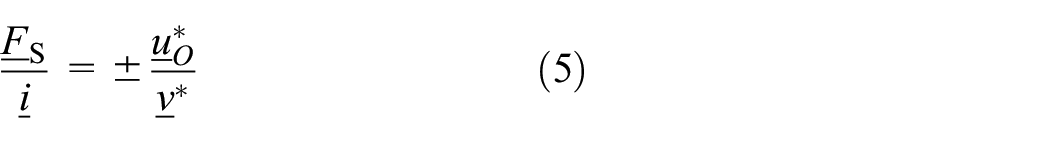
The reciprocity property can be checked by hand of two sample experiments. Given the system E in Figure 1 with six ports, two ports are selected first. In Figure 1, these are ports 3 and 6; the remaining ports can be open- or short-circuited. These boundary conditions have to be retained in both experiments. In the first experiment, a sinusoidal voltage with the complex magnitude, expressed by the underline,
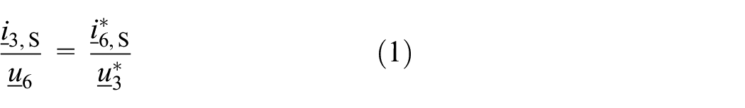

Reciprocal experiments at an electrical system.
This law indicates the reciprocity of a passive linear network. It is not limited to electrical systems but also applies to systems incorporating various physical structures.
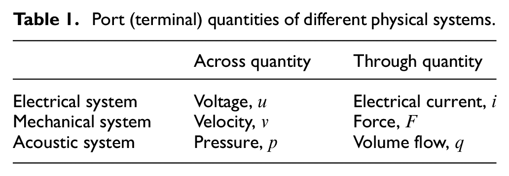
Analogous to the electrical system E, the experiments can be performed on a passive electromechanical system with reciprocal transducers to detect reciprocity relations. As stated for electrical systems, the electromechanical system consists of interconnected reciprocal subnetworks. Besides the electrical elements, these are, for example, compliances, masses, reluctances, acoustical masses, and acoustical compliances, as well as space-limited continua. The across and trough quantities in different physical subsystems in this article are listed in Table 1. Reciprocal transducers relate consistently pairs of trough and across quantities of different physical structures to each other (Lenk et al., 2010). These, so-called “passive,” transducers between two ports do not include internal energy sources, that is, the total delivered power at one port is provided by the other port.
Port (terminal) quantities of different physical systems.
With regard to an arbitrary passive linear electromechanical system, reciprocal experiments can cover arbitrary electrical and mechanical ports, as emphasized by Marschner et al. (2013). In the first experiment, for two selected ports, a voltage
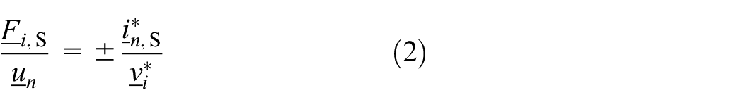
For electromechanical transducers, further reciprocity relations can be derived as a subset of all the transfer functions
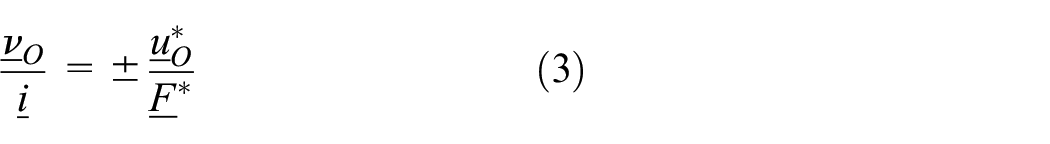
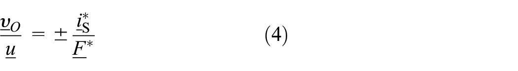
where the plus sign is related to magnetic transducers and the minus sign to electric transducers. The linked pairs of flow and differential quantities are marked in Figure 2. The indices S and O denote short circuit and open circuit, respectively. In the transducer, only reciprocal processes are allowed in accordance with thermodynamics. For such transducers, the separation of losses into the surrounding network out of the transducer succeeds. Electrical and magnetic transducers fulfill this condition (Lenk et al., 2010).
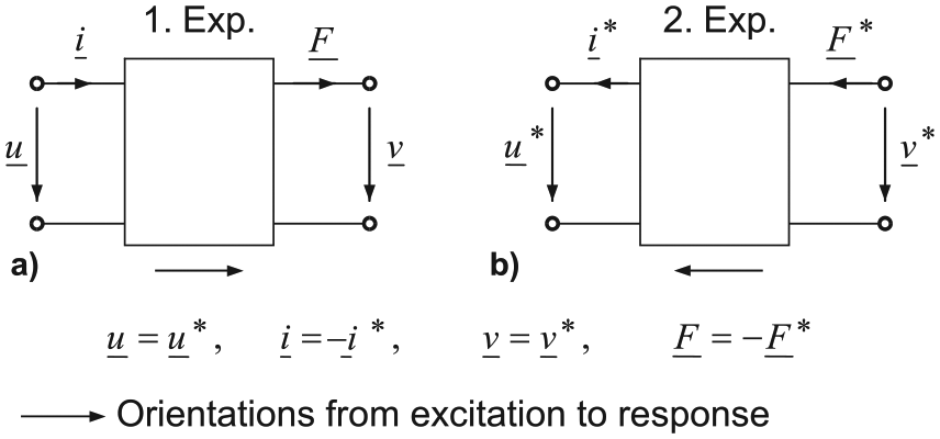
Reference arrow directions of electromechanical transducers for (a) electrical excitation and (b) mechanical excitation.
In metrology, the calibration of accelerometers is a classic application of the reciprocity relations. A mechanical calibration source is not required, but any arbitrary additional electromagnetic transducer can be used. This application is analyzed in the second part of the article.
The application of reciprocity relations furthermore proves to be advantageous when continua are part of the system. In 1926, Schottky applied the reciprocity theorems of classical vibration theory for the determination of reception and transmission properties of electroacoustic transducers. Thus, the effect of an impacting quasi-spherical wave on a surface element could be calculated from their emission efficiency. Schottky illustrates the methodology on the example of an electrodynamic horn speaker which prefers low frequencies when it is used as receiver. The law led to the mathematical theory of the receiving cone. The actuality of the methodology is demonstrated by an electroacoustic example.
In the last part of the article the linearity of an electromechanical system is checked by hand of reciprocity relations, where in addition the excitation signal magnitudes are increased. When the related experiments approve the reciprocity, the system behaves linearly. When the reciprocity relations are violated, the system behaves non-linearly. A simple model is applied to describe the source of nonlinearity.
Reciprocity of piezoelectric transducers
Reciprocity of piezoelectric materials is explicitly included in their field equations
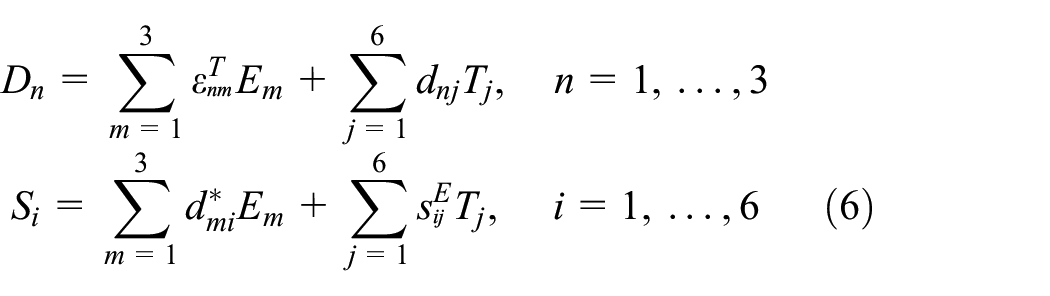
where D is the electric displacement, ε the permittivity, E the electric field strength, T the mechanical stress, S the mechanical strain, and s the elastic compliance. The piezoelectric coefficients
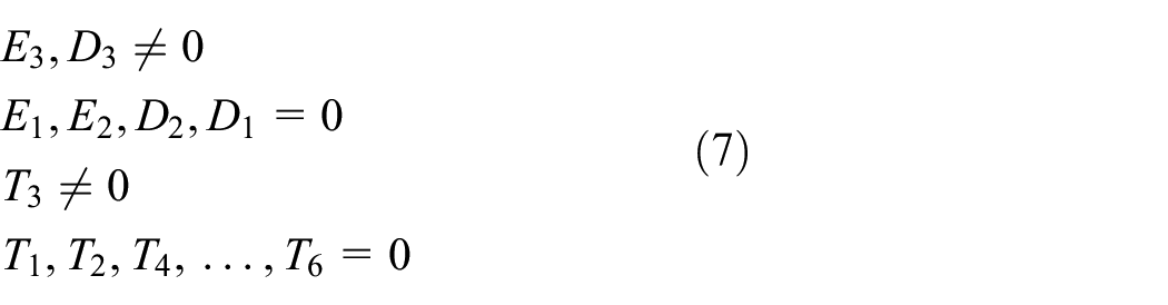
Application of boundary conditions and integration gives a device description. It is shown below how the reciprocity of the constitutive field equations is transferred to the device equations. In case of a free thickness oscillator, for example, see Figure 3, only the fields in direction 3 are non-zero
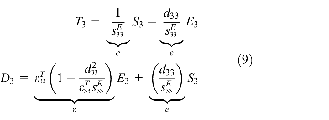
and equation (6) reduces to
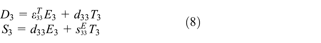
or, with the elastic coefficient c and the piezoelectric modulus e to
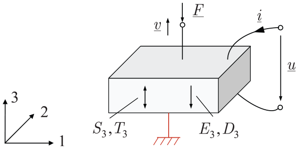
Free piezoelectric thickness oscillator (Lenk et al., 2010).
Integration of uniform fields and transitions to complex quantities gives voltage
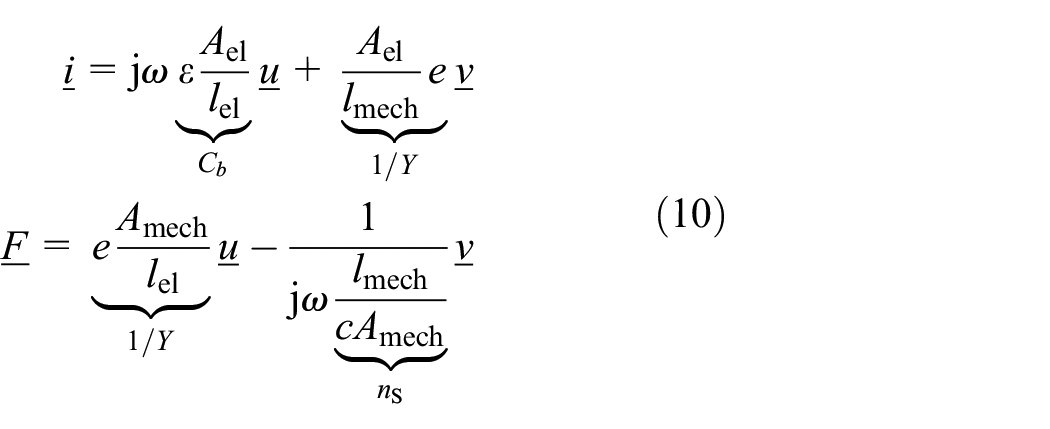
Circuit interpretation of equation (10) leads to the well-known circuit in Figure 4 (Lenk et al., 2010).
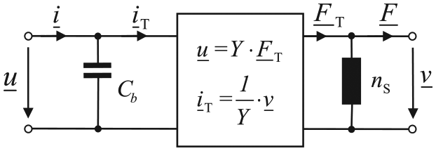
Equivalent circuit of a piezoelectric transducer.
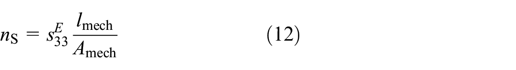
For free thickness oscillators, the network parameters can be analytically determined: the transduction coefficient
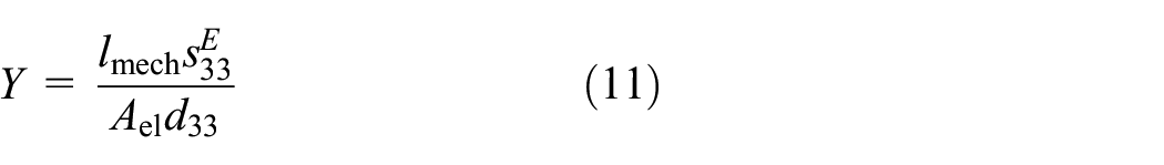
with the thickness lmech working in actuation and sensing direction, respectively, area Ael of the piezo block and electrodes, the piezoelectric constant d33, the elastic constant
and the mechanically blocked capacitance
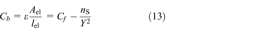
with permittivity ε. The mechanically free capacitance Cf differs from Cb by the transformed compliance. The boundary condition–dependent network parameters for other oscillator types can be found, for example, in Lenk et al. (2010).
The reciprocity of this transducer device or two-port is checked exemplarily by means of equations (2) and (3). To verify equation (2), the transducer in Figure 4 is excited with a voltage source and a velocity source subsequently. These difference quantities act directly at the transformer core. All flow quantities of the transducer core are directly accessible if the related other physical domain is short-circuited or blocked, respectively. The first reciprocity relationship can thus be read from the transducer core equations
The negative sign is due to the reversed direction of the short-circuit current compared to the defined direction of iW.
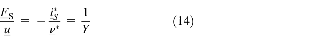
To prove the reciprocity relation (3), a current
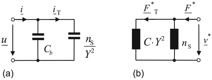
Transformation of piezoelectric transducer components in Figure 4 to prove reciprocity equation (3). (a) Transformation of the short-circuit compliance and (b) transformation of the blocked capacitance.
Considering the first experiment, the electrical side of the transducer results in the relationship
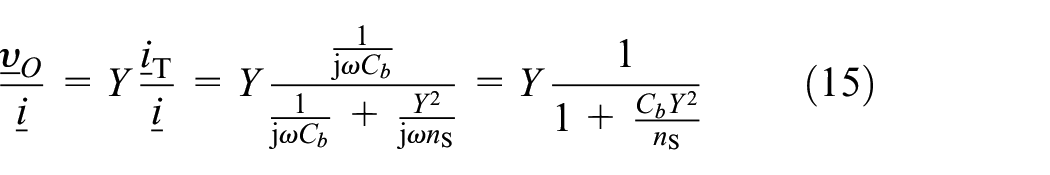
and, considering the second experiment, at the mechanical side with
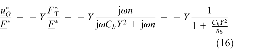
From equations (15) and (16) follows equation (3) for electric transducers
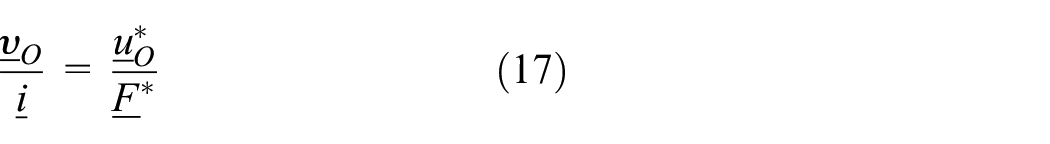
The other reciprocity relationships can be checked similarly.
Reciprocity of piezomagnetic transducers
One-dimensional magnetomechanical transducer
When a magnetostrictive rod resides as solenoid core freely (stresses T1, T2, T4, …, T6 = 0) at the transducers center, as investigated by Kellogg et al. (2005), a one-dimensional (1D) translational transducer model—similar to the piezoelectric transducer—can be derived. Considering the field quantities stress T and magnetic field strength H to be independent variables, the total differentials
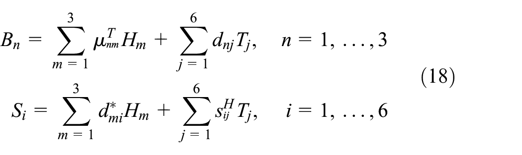
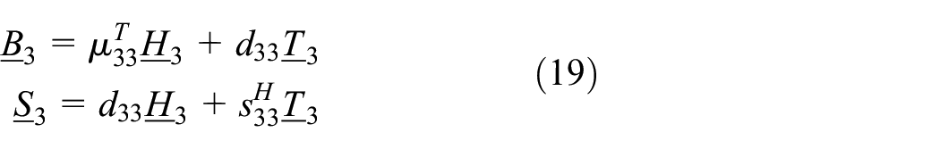
give the linear constitutive equations for flux density B and strain S in a piezomagnetic body at an operating point. When H is applied in parallel to T, then equation (18) yields for complex quantities
with permeability
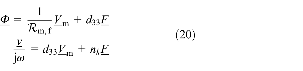
in the complex domain. Equation (20) includes the body properties’ compliance
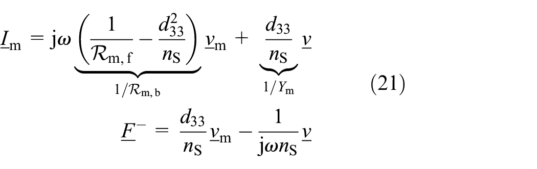
Equation (21) characterizes a piezomagnetic transducer in the mechanical domain by its compliance nS and in the magnetic domain by its magnetic reluctance
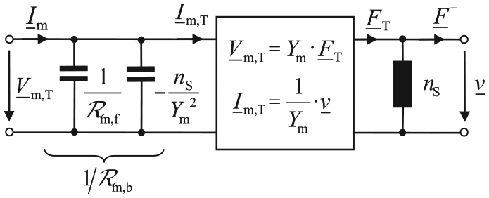
Translational magnetomechanical two-port model of a piezomagnetic transducer.
1D electromechanical transducer utilizing a solenoid
A long and thin solenoid coil (radius
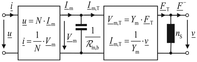
Model of a piezomagnetic transducer residing as solenoid core.
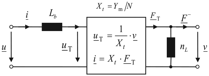
Electromechanical model of a piezomagnetic transducer after reluctance transformation into Lb and transducer combination in Figure 7.
Equation (5) can be easily checked. In order to resolve this equation, an electrical current is applied to the electrical port. The current is transformed into
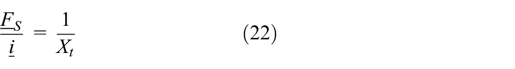
In a second experiment, a velocity source
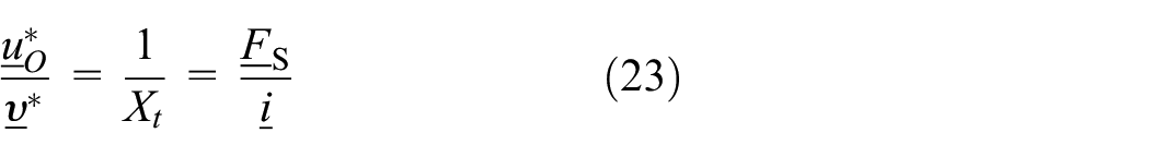
The other reciprocity relations can be proved similarly by application of the network theory.
Piezomagnetic unimorph
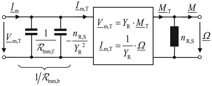
Two-layer piezomagnetic elements with a magnetic and a non-magnetic layer are being used in bending actuators or sensors. In contrast to volume transducers, two-layer elements achieve significantly larger displacements. The dynamic magnetomechanical behavior of such a unimorph can be described by the equivalent circuit in Figure 9, as it is derived by Marschner et al. (2014b). The transduction coefficient YR relates bending moment
Piezomagnetic unimorph core in a solenoid.
In Marschner et al. (2014a), the reciprocal transducer properties of a piezomagnetic unimorph were investigated. The unimorph with the reluctance
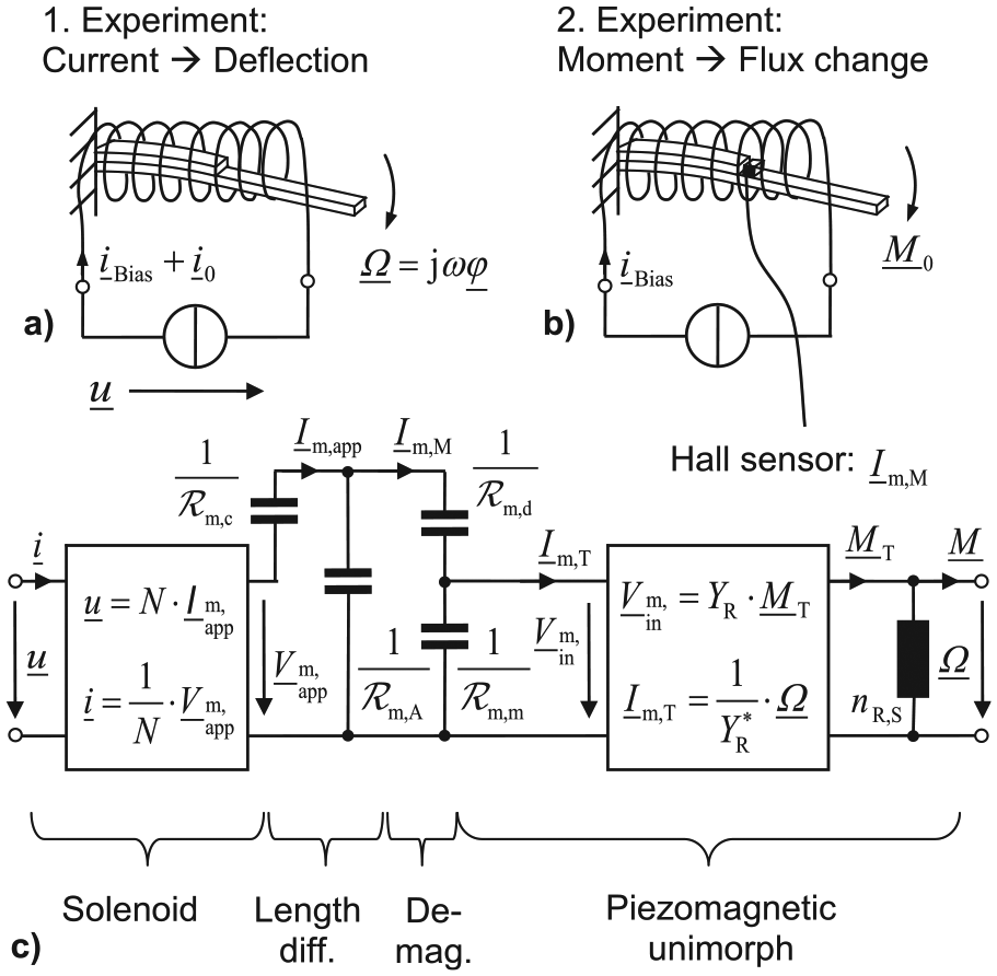
(a) and (b) Performed reciprocal experiments. (c) Rotational electromechanical model of a piezomagnetic unimorph core in a solenoid, as derived in Marschner et al. (2014a). The length difference between coil and magnetostrictive patch constitutes a magnetic voltage divider (
Application of the reciprocity relationship for the calibration of acceleration sensors
A classic application of the reciprocity relations is the calibration of accelerometers. The calibration requires no mechanical calibration source, but an arbitrary additional electromagnetic transducer as depicted in Figure 11. Both transducers, the magnetic transducer and the accelerometer, are connected via mass m3.
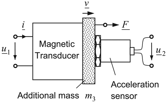
Acceleration sensor calibration setup.
The construction of the standard magnetic transducer is depicted in Figure 12. Two masses are involved: the mass of all components, which move with the housing mm,h, and the total mass of all components, which move with the vibration table mm. From this magnetic transducer, the mechanical input impedance
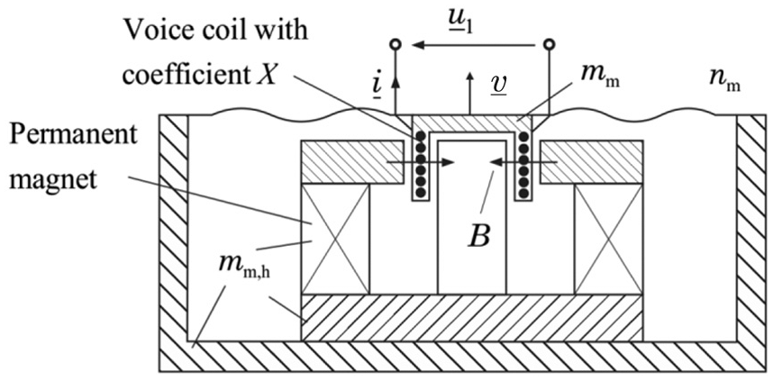
Magnetic transducer setup.
A piezoelectric accelerometer is mounted exemplarily to the vibration table. Piezoelectric accelerometers contain a piezoelectric ceramic as electromechanical transducer element. This ceramic can be used in the form of a circular-shaped element (for thickness oscillators) or a rectangular element (for bending and shear oscillators). The basic structure of an accelerometer with circular-shaped element is shown in Figure 13. Upon application of forces in the drawn direction, an electrical voltage is generated between the metallized electrodes. The magnitude of the no-load voltage
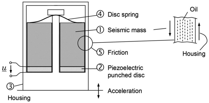
Piezoelectric acceleration sensor construction.
The equivalent circuit of the mechanical components of the accelerometer in Figure 14 shows the compliances of the disk spring and the piezoelectric ceramic, which act in parallel. The equivalent circuit shows that the sensor exhibits bandpass properties. Low-frequency accelerations do not have an effect on the seismic mass.
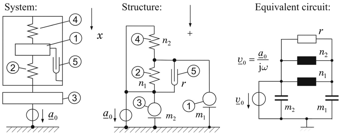
Mechanical part of a piezoelectric acceleration sensor, its structure, and circuit description; the force on n1 determines the transduced voltage.
The completed equivalent circuit of the calibration system is depicted in Figure 15. All masses establish a virtual connection to the inertial frame. The mass of the sensor is considered to be a part of the transducer system. Thus, impedance

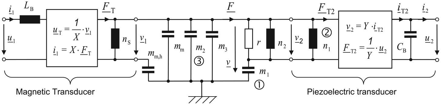
Equivalent circuit of the piezoelectric transducer calibration setup in Figure 11.
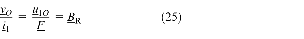
It is the goal of the calibration to determine the transfer function
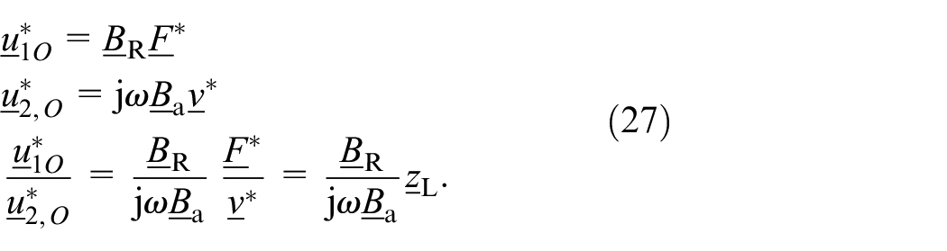
The calibration utilizes the electromechanical reciprocity relation of the magnetic transducer
Calibration requires two experiments, as shown schematically in Figure 16. First, an electric current
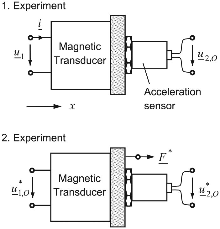
Acceleration sensor calibration experiments.
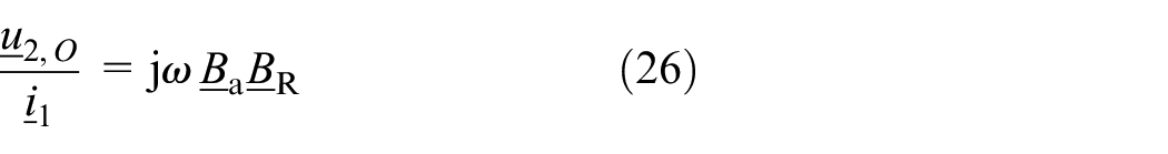
In the second experiment, an external force
Typically, the calibration system is designed in a way that good approximation of
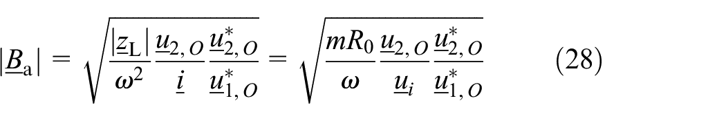
Since these quantities can be measured simple, fast, and highly accurate, an efficient calibration method results (Lenk et al., 2010).
Application of the reciprocity relationship for the calibration of measurement microphones
A currently indispensable application of reciprocity is the primary calibration of laboratory standard microphones. This is carried out by the national metrological institute (e.g. the Physikalisch Technische Bundes-anstalt of Germany) to represent the unit of sound pressure Pascal (Pa). The unit is passed from these primary-calibrated standard microphones in turn to all to be calibrated microphones of the country by means of a comparative method.
The microphone calibration by the reciprocity method—described in its principles by MacLean (1940)—is currently the method by which the lowest measurement uncertainties can be obtained. There are two main reasons:
The first sound pressure measurement is based on the measurement of mechanical and electrical quantities which is possible with very high accuracy.
The transfer function of measuring microphones depends on the acoustic boundary conditions under which the microphone is used.
Only with the help of the reciprocity procedure, the direct calibration for the metrological relevant cases—pressure chamber (DIN EN 61094-2:2009, 2009), free field (DIN EN 61094-3:1995, 1995), and diffuse sound field (Vorländer, 1996)—is currently possible.
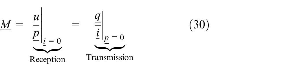
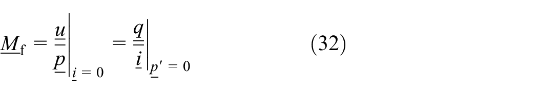
The basis for the calibration is the reciprocity of electrostatic measurement microphones. As a prerequisite, they need to be operated in their sufficiently linear region. Figure 17 shows the definition of the electric and acoustic quantities for the electroacoustic two-port “microphone.” These are voltage u and current i at the electrical port as well as sound pressure p—averaged over the membrane surface—and acoustic volume flow, generated by the entire membrane, at the acoustic port. With these quantities, the electroacoustic circuit of the microphone in Figure 18 for the linear region can be specified. As the impedance matrix of the two-port network follows
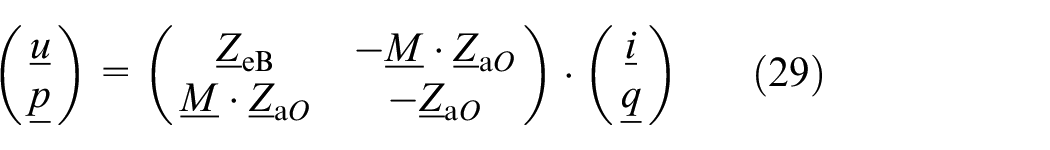
where
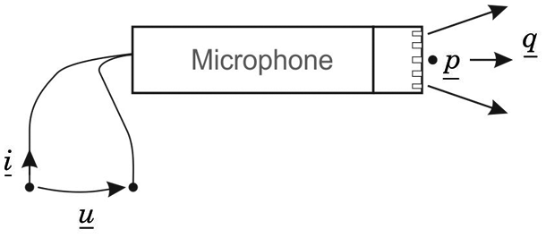
Electric and acoustic parameters on electrostatic measurement microphone.
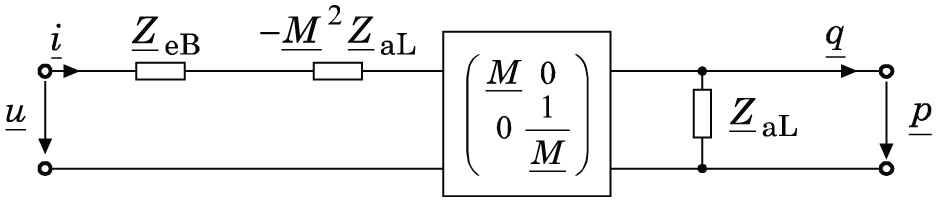
Electro-acoustic circuit of the microphone.
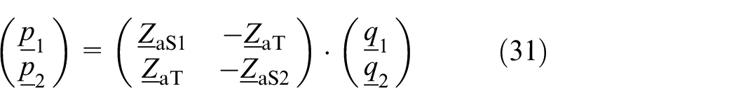
For the calibration, one microphone is used as a transmitter and one microphone as a receiver (hereinafter distinguished by subscripts 1 and 2), as shown in Figure 19. The acoustic transmission path between the sound flow
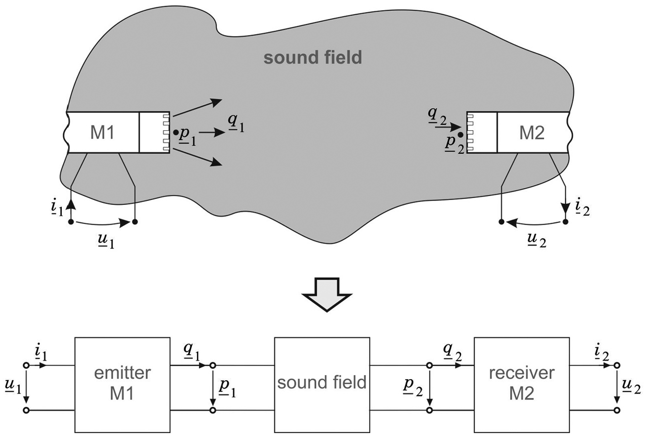
Microphone calibration setup.
Figure 20 shows the resulting circuit of the entire calibration system.

Equivalent circuit of the calibrator.
Different acoustic impedance matrices result, depending on whether the calibration takes place in the pressure chamber, in the free field, or diffuse sound field. Subsequently, the next steps illustrate free-field calibration. For the free-field calibration according to DIN EN 61094-3:1995 (1995), the free-field transfer function
is introduced with respect to the sound pressure
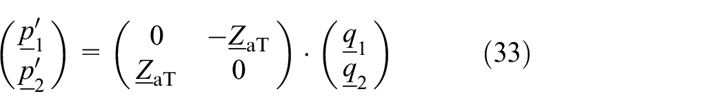
with the acoustic transfer impedance
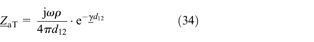
which describes the propagation of sound in a free field. Here,
Together with the known acoustic transfer impedance
of the microphones can be calculated.
In summary, only measurements of voltage, current, and effective distance as well as knowledge of frequency, air density, and sound velocity were necessary for the determination of the microphone transfer functions. Using reciprocity calibration, extremely low measurement uncertainties for acoustics of ≤0.05 dB are reached in the frequency range of 31.5 Hz to 8 kHz (free-field and pressure chamber calibration; Bork et al., 2007). Even in the lower ultrasonic range of 20–160 kHz, measurement uncertainties of less than 0.2 dB were achieved (Bouaoua, 2008) for the free-field calibration of 1/4″ microphones. There is currently no alternative method which achieves a similar low measurement uncertainty and which is suited for the calibration in the pressure chamber, in the free field, and in the diffuse sound field.
As a future supplement to reciprocity, the use of optical measurement methods for the calibration of microphones is subject of this research (see Koukoulas et al., 2008; Theobald et al., 2002). These methods have not yet achieved the lowest measurement uncertainties of reciprocity.
Application of the reciprocity relations for linearity check of systems
Since linearity is one prerequisite of reciprocity, an obvious way to perform a check on linearity of a system results in utilizing reciprocity relations. A structure is analyzed metrologically in a way whether the component arrangement fulfills the reciprocity relation. At sufficiently small signals, one expects consistent reciprocal relationships if the system behaves linearly. A fast subsequent performance of the two experiments eliminates cross sensitivities and parameter drifts most widely. If for larger signal magnitudes an increasingly growing deviation is found, it is ultimately due to nonlinearities in the system. Here, the source of nonlinearity and its strength cannot be initially identified. This method allows a check for sufficient linearity using a configuration in which only one branch with respect to its linearity is unknown. Since under correct boundary conditions the reciprocity yields to identical signal forms, the check of the linearity can be traced back to a time measurement.
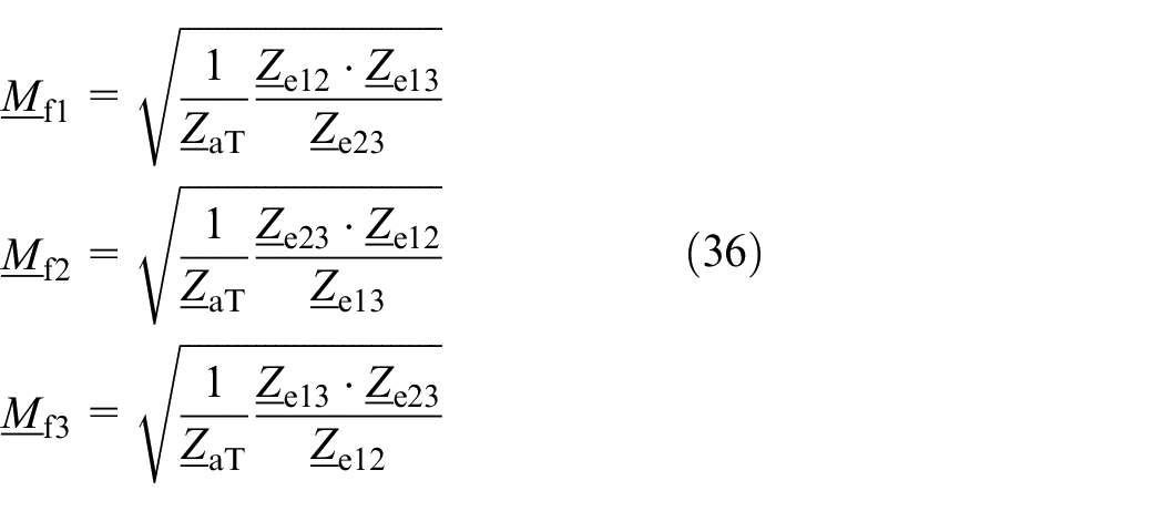
The method is demonstrated exemplarily by the coupling of two piezoelectric transducers by a rod, as depicted in Figure 21. It is assumed that the rod shows sufficient linear behavior. In a first experiment, transducer 1 is excited with a low-voltage magnitude, which is in the linear region of the transducer. At transducer 2, a transient short-circuit current signal is measured. By the evaluation of the transmitted voltage and the received current signal, the transit time
Coupling of two piezoelectric transducers with a rod.
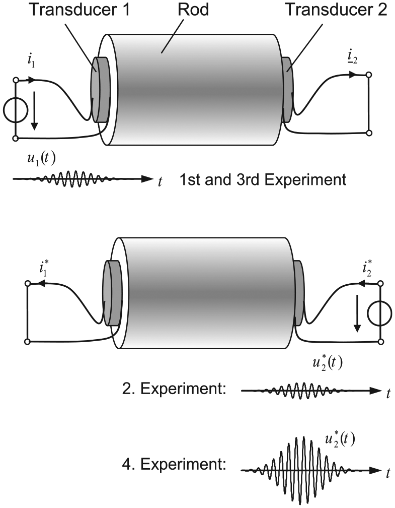
Then, the third and the fourth experiments are performed subsequently. The third experiment is identical to the first experiment. In the fourth experiment, the excitation voltage magnitude at transducer 2 is increased. Therefore, transducer 2 leaves the linear operation range and the prerequisite for the reciprocity is violated. This, in turn, leads to a change in the transit time
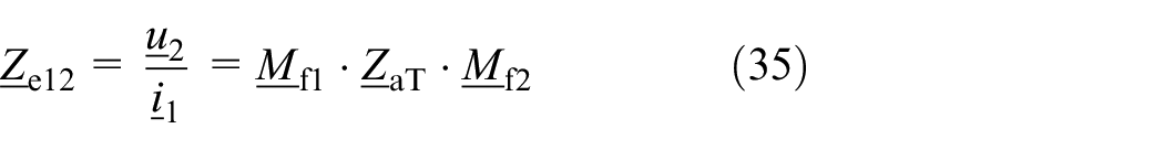
The magnitude-dependent nonlinearity is modeled with an additional quadratic factor A in the transducer relation of the equivalent circuit in Figure 22. When the experiments are performed below the rod’s first natural frequency, the rod can be modeled by a T-circuit consisting the rod’s compliance and mass. The factor A is determined by simulation experiments using the equivalent circuit where the time delay difference is reproduced. The basic idea is to keep all parameters equal in both measurements, except one. When the measurements can be described this way, then the source of the nonlinearity is found. This way, the nonlinearity can be captured with little effort.
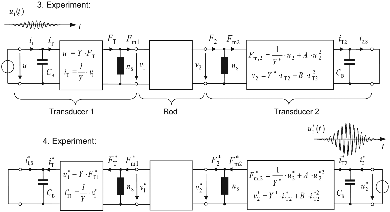
Equivalent circuit of the coupled piezoelectric transducers due to the amplitude-depending time delay difference the nonlinearity can be assigned to coefficient A.
Summary
Reciprocal linear time-invariant systems are an essential basis in electromechanical metrology. The article shows some examples for calibration, reduction in measurement uncertainty, and checking of nonlinearities, where reciprocal relations of time-invariant linear networks are utilized in different ways. This applies in particular for linear systems, which include continuously distributed media.
Footnotes
Acknowledgements
The authors would like to thank Prof. Albrecht Reibiger (Technische Universität Dresden) and the editorial reviewers who volunteered their time and expertise to read and critique the article and for their constructive comments.
Declaration of Conflicting Interests
The author(s) declared no potential conflicts of interest with respect to the research, authorship, and/or publication of this article.
Funding
The author(s) received no financial support for the research, authorship, and/or publication of this article.