
Abstract
The present work explores the generation of two-dimensional steady-state flexural waves that are non-reflective on a thin rectangular plate with free boundary conditions when excited by two macro-fiber composites (MFCs). The voltage signals to the MFCs have a frequency lying halfway between two adjacent resonant frequencies with a phase difference of
Introduction
Waves with their ubiquitous traveling nature have numerous examples and applications in both the organic and inorganic worlds. In the present work, we broadly classify these waves into transient traveling waves and steady-state traveling waves. In a water body, a disturbance propagating away from its point-of-origin is a good example of the first type of traveling wave. These waves are evanescent in nature and change their course of travel if there is a hindrance in their path. Such wave type are often utilized for various applications such as structural health monitoring (Fromme et al., 2006), stress analysis (Frikha et al., 2011; Shi et al., 2013), event localization (Poston et al., 2015; Schloemann et al., 2015) and dispersion compensation, to name a few.
Steady-state traveling waves are the other type of traveling waves. The traveling feature of these waves is perpetual and steady-state nature in comparison with the transient characteristics of the transient traveling waves. Visually, it “appears” as if these waves are not affected by the boundaries of the structures, however in reality, the progressive motion is the resultant response after multiple interactions with its boundaries. Such behavior is exhibited in the undulations of the flagella or cilia of micro-scale organisms (Machin, 1958; Stone and Samuel, 1996; Taylor, 1951), the fins or tails of aquatic animals (Fish, 1996; Long et al., 1994; McHenry et al., 1995). The steady-state traveling waves of these bio-examples generate propulsive force (Drucker and Lauder, 1999) and manipulate drag force (Barrett et al., 1999; Fish, 1996) by disturbing fluid boundaries, and play a vital role in bio-mimicking robotics (Erturk and Delporte, 2011; Jones et al., 2014; Lauder et al., 2011) and bio-inspired designs of marine and aerospace vehicles (Bushnell and Moore, 1991; Fish, 1998; Koike et al., 2004). As a step towards the integration of these bio-dynamics into engineering systems, the present research investigates the concept of two-dimensional (2D) steady-state traveling wave generation in planar structures. As steady-state traveling waves are the focus of this article, they are refereed as traveling waves in the rest of the article.
Despite such a wide range of applications, no significant effort has been made to understand the passive manipulation of structural impedance to generate steady-state traveling waves in continuous media. To emulate traveling wave behavior, some researchers working on bio-robotics have used multiple time-synced actuators to discretize the wave patterns (Wang et al., 2008, 2009) and others have actively manipulated the boundary conditions of continuous systems to generate a complex combination of standing waves (Kancharala and Philen, 2014a, 2014b). These approaches either do not make use of the intrinsic vibratory properties of the structure to produce traveling waves, or require a large number of actuators and sensors for feedback control algorithms. The present work exploits the characteristic vibrations of continuous solid structures to develop traveling waves with the least number of actuators and limited control effort.
The traveling wave generation approach in this article is an extension of the two-mode excitation technique (Gabai and Bucher, 2009, 2010; Minikes et al., 2005) or the impedance-matching efforts (Gabay and Bucher, 2006; Loh and Ro, 2000) previously carried out in one-dimensional (1D) systems. In these previous studies, a string or a beam is excited simultaneously by two actuators at a frequency halfway between two adjacent natural frequencies with a phase difference of
The present work is broadly divided into three parts: the first part discusses the modeling approach pursued to simulate plate dynamics with piezoelectric patches attached to the plate. The second part focuses on model updating and model validation through experimental modal analysis. In this section, the eigenvalues and eigenvectors of the damped plate finite element (FE) model are compared with experimental results. Once the plate model is validated for a single input response, traveling wave generation is addressed in the third part. Experimental and numerical responses of the plate are compared with each other when the plate is simultaneously excited with two piezoceramic patches. Additionally, multiple approaches are developed to differentiate and categorize the plate behavior into standing or traveling waves, and the effects of frequency and location on the quality of the traveling waves are discussed.
Part I: Modeling plate dynamics
Consider a homogeneous, isotropic, linear elastic plate, with four piezoelectric actuators perfectly bonded to it, as shown in Figure 1(a). The length, the width and the thickness of the plate are denoted by
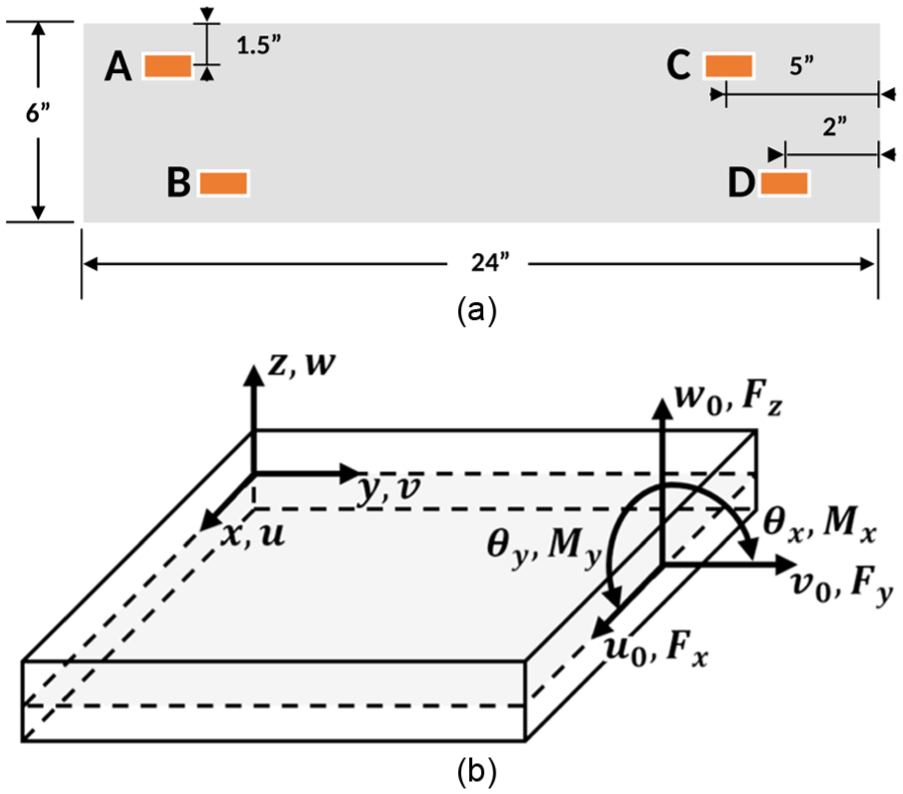
Experimental setup: (a) rectangular plate with MFCs; (b) forces and moments acting on a plate element.
The focus of this article is to investigate traveling waves at relatively low frequencies (up to 3000 Hz). At such frequencies the effects of the adhesive bonding layer between the plate and the piezo patches are negligible (Albakri and Tarazaga, 2016), and hence, those sections of the plate covered with piezo patches are considered as a composite structure. With this assumption, the classical lamination theory is adopted to obtain the equivalent material characteristics for these composite sections. Furthermore, since traveling waves are, in general, generated in thin plates, the first-order shear deformation theory (FSDT) has been adopted to define the displacements in the structure. Based on the aforementioned assumptions, the displacement field in the plate is defined as
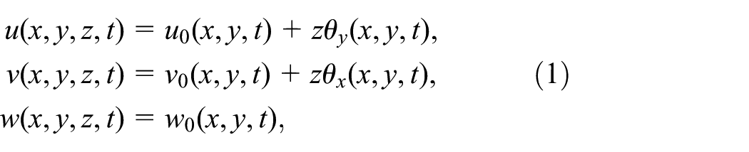
where
Translational and rotational degrees of freedom are split throughout the derivation of the governing equations and the formulation of the FE as follows
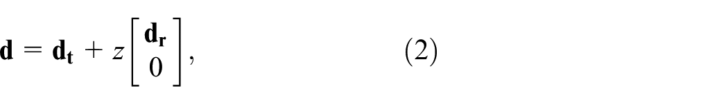
where
To avoid the issue of shear-lock associated with shear deformations, a reduced integration rule is used to evaluate the transverse shear strains (
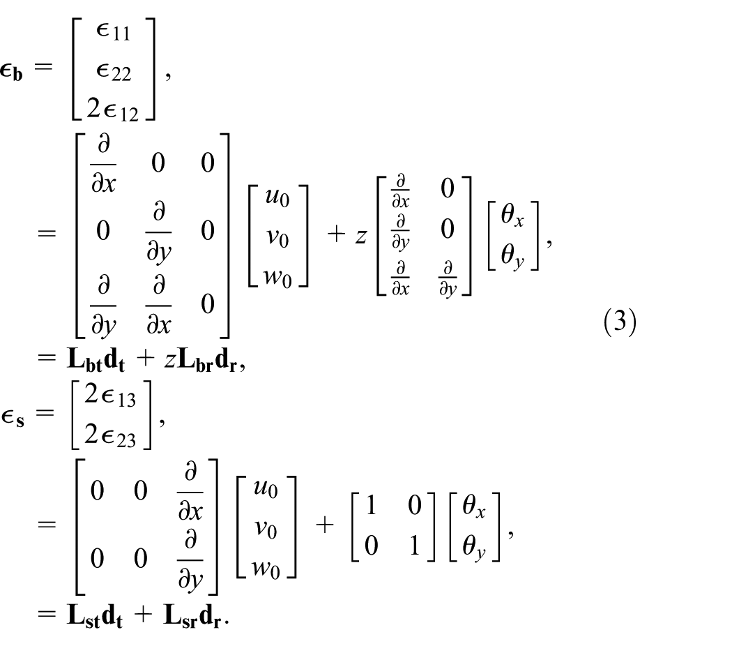
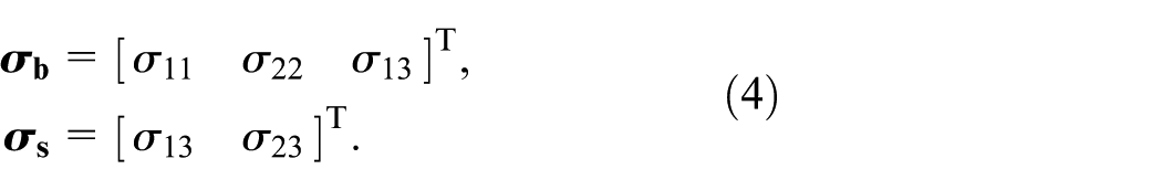
Following the same notation, the state of the stress at any point in the plate is described by the in-plane stresses (
The plate is assumed to be made of homogeneous, isotropic, linear-elastic material with the following constitutive relations
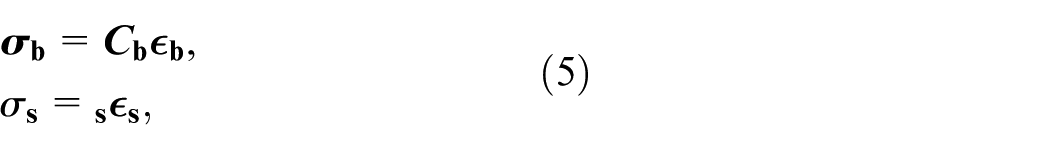
where
Assuming linear piezoelectricity, the constitutive equations for the piezoelectric actuators are (Leo, 2008)
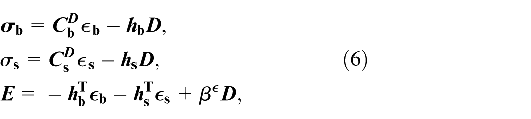
where
Based on the aforementioned assumptions, the kinetic energy of the piezoelectric plate system can be written as follows
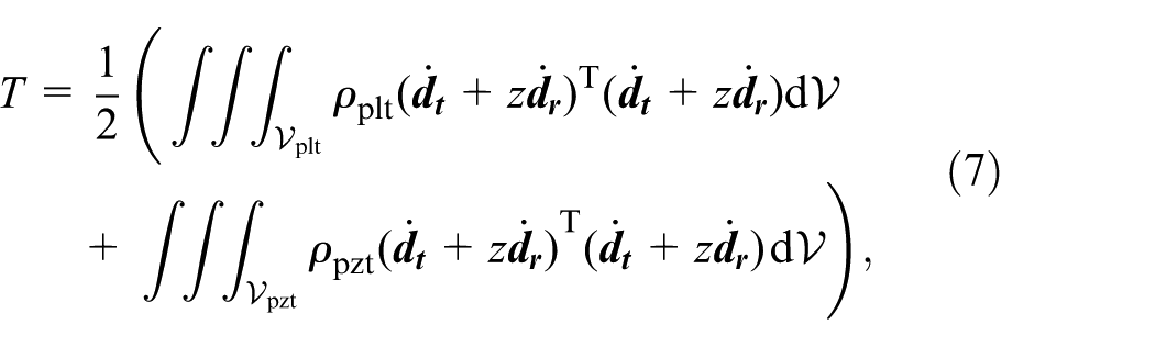
where
Following the Helmholtz free energy definition for piezoelectric materials, the potential energy functional of the system, including the strain energy and the work done by external forces, can be expressed as
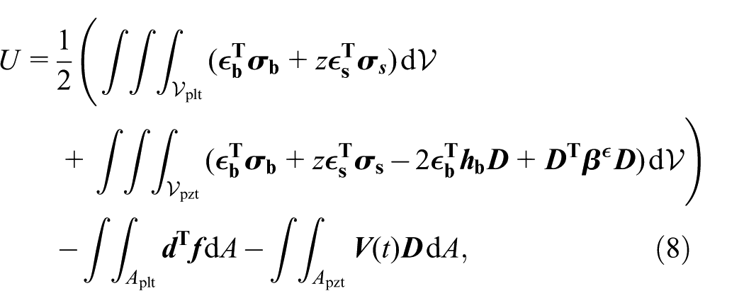
where
Using eight-noded isoparametric quadrilateral elements to discretize the plate, the displacement vectors, associated with the ith
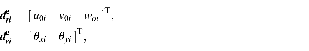
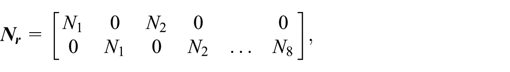
On the element level, the displacement field at any point within the element can be defined in terms of the nodal displacement vectors,
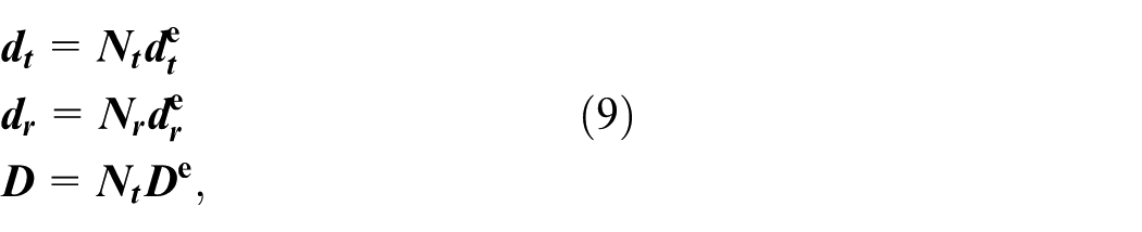
where
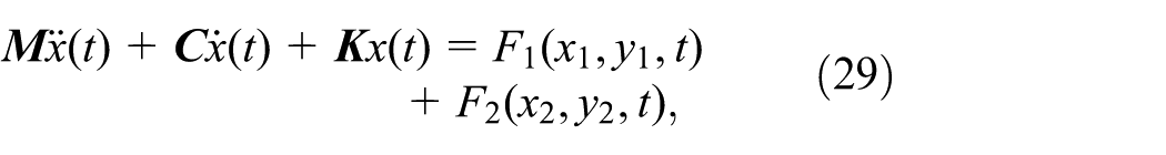
and
where
Upon substitution into equations (7) and (8), energy functionals can be written as
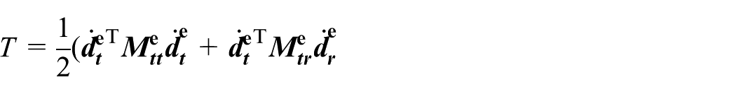

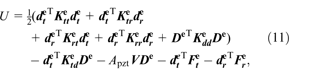
where all element matrices are defined in Appendix 2.
Applying Hamilton’s principle, the equations of motion for the plate with the piezoelectric actuators are obtained as follows
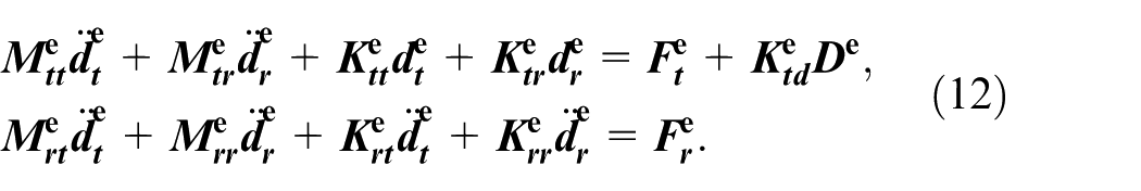
An additional equation can also be obtained for the elemental electric displacement degrees of freedom,

Substituting equation (14) into equation (13) and assembling the elemental matrices yields
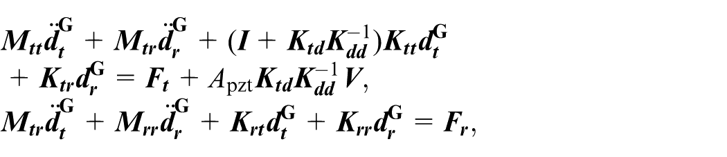
where
Part II: Modal testing of the plate
In the previous section, the dynamics of the plate are modeled through a finite element approach and this section validates the results of this model experimentally. A single-input-multi-output (SIMO) modal testing procedure is followed to extract eigenvalues and eigenvectors of the plate. Furthermore, the damping characteristics of the plate are experimentally acquired and the FE model is then updated to include damping. The various steps followed in this modal testing and validation phases are discussed in the following sections.
Experimental setup
The experimental work in the present article adopted an aluminum plate of dimensions
Material properties for the augmented PZT-adhesive-beam system (Simulia, 2012).
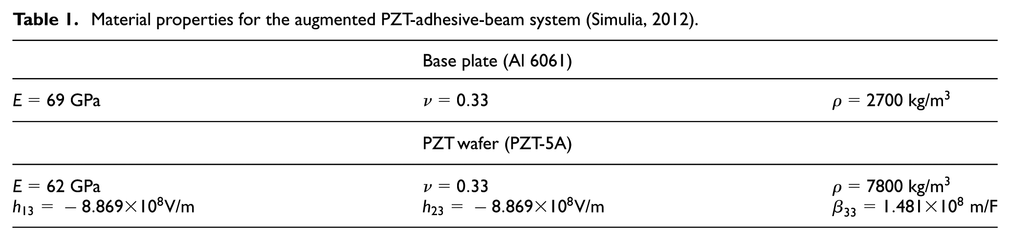
Experimental setup: (a) a rectangular plate is suspended in air to simulate a free boundary condition; (b) locations of four MFCs bounded on to this plate are shown w.r.t. the plate dimensions; (c) a scanning laser vibrometer measures the response of the plate as it is excited by these MFCs.
The plate is suspended in the air with two pre-tensed fishing lines to replicate an overall-free boundary condition (Figure 2(a)). The forces on the plate on account of the support strings are hence neglected in the current analysis. The strings are placed to balance the plate horizontally and at the same time not to interfere with the MFCs bonded to the bottom surface of the plate. When one or more of the MFCs is actuated, the plate is excited, and the resulting vibrations are measured by scanning the top surface of the plate using a Polytec Scanning Laser Doppler Vibrometer (SLDV). To facilitate model validation, 493 scan points are imported into Polytec SLDV software from the FE mesh; this enables an easier and more accurate comparison of experimental and numerical results.
Firstly, single input single output (SISO) modal analysis of the plate is performed through multiple frequency-sweep tests to generate Frequency Response Functions (FRFs) and experimental Operational Deflection Shapes (ODSs). In these tests, MFC A is excited with a sine-sweep signal of frequency ranging from 10 to 3000 Hz and a constant amplitude of 14 V. The SLDV measures the out-of-plane velocity of the plate at each of these 493 scan points and computes the corresponding FRFs w.r.t the input voltage supplied to the MFCs. To reduce noise effects, 20 FRFs are generated and averaged at each point. This data is further analyzed to extract experimental eigenvalues, eigenvectors, and damping parameters. These results are discussed in the next section and later this setup is used to generate traveling waves in the plate.
Operational deflection shapes and eigenvectors
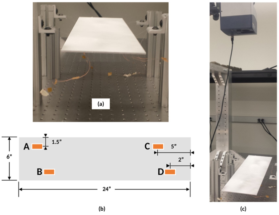
The Polytec software processes the time-based vibration signal into the frequency domain in two ways. These are the
The input and output noise effects are seen in these signals; while
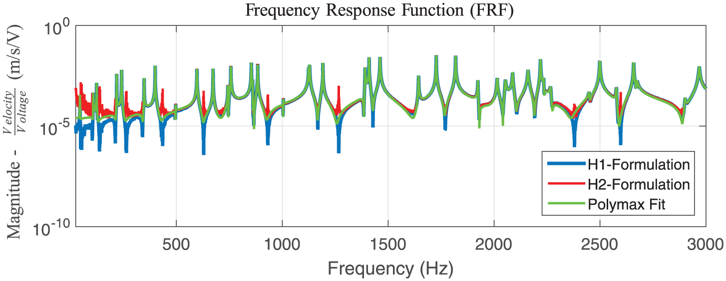
Experimental FRFs are compared against the LMS PolyMax fit.
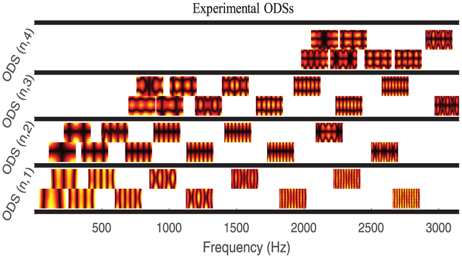
Experimental ODSs as measured by the Polytec SLDV.
Hence, to extract mode shapes (or eigenvectors) from these FRFs, we make use of the PolyMax algorithm in the LMS TestLabs software to fit the frequency data. This polyreference least-squares approach computes a stabilization diagram based on complex frequencies, damping and participation factors obtained from the FRFs. Complex eigenvectors are extracted by least-square fits of smaller frequency intervals using both
Additionally, the experimental damping coefficients (
Proportional viscous damping parameters
The earlier sections on the modeling efforts of the plate dynamics with the piezoelectric patches discussed the derivation of mass
The dynamic FE model of the plate including the effect of viscous-based damping can be represented by

The non-trivial complex solution of this equation is of the form

The unknown parameters
As the mode shapes of this system are real-valued, the real and imaginary components of this equation are uncoupled and can be rewritten as
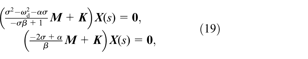
Both of these equations, which are in the form of a generalized undamped eigenvalue problem, should be satisfied simultaneously; the coefficients of the mass matrices are simultaneously equal to the undamped natural frequency
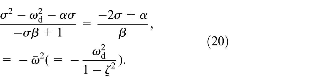
With the help of these two relationships, the undamped natural frequencies (
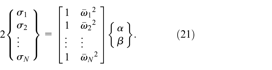
This equation has two known quantities
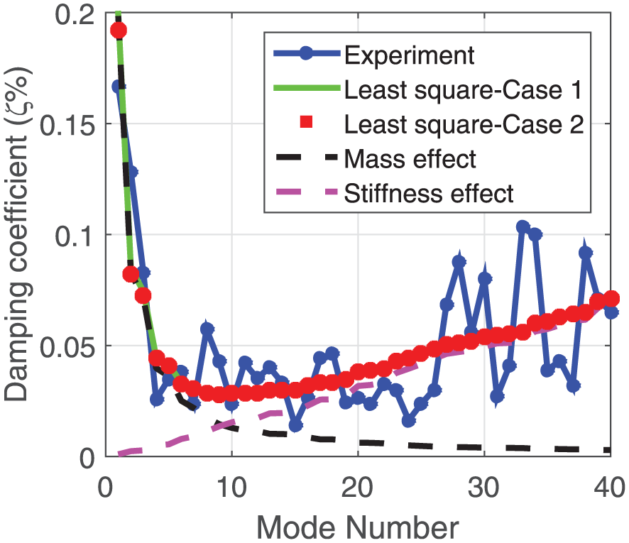
Experimental damping estimates based on the
As the proportional damping coefficients estimated through both cases are very close to each other, the coefficients estimated in Case 1 are used in the rest of the article. Based on these values, the complex eigenvalue problem is solved in the next section.
Complex eigenvalue problem
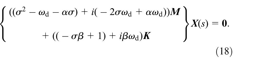
The previously developed FE formulation of the plate is updated with the proportional damping values computed in the previous section and this results in

The eigenvalue problem arising from this set of equations is a complex equation and can be observed when

This equation results in complex eigenvalues and complex eigenvectors, which are solved in Matlab using the
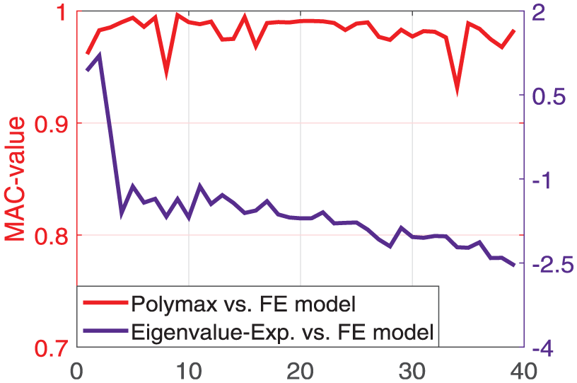
Simulated Eigenvalues and Eigenvectors of the damped plate model are compared against corresponding experimental values through the % error in eigenvalue prediction (red) and MAC (purple) respectively .
The updated FE model is able to predict eigenvalues with a maximum error of 2.5% for the entire bandwidth. Other than the first two eigenvalues, the FE model eigenvalues are in general larger than the experimental eigenvalues, and the error gradually increases with the number of modes. Such a trend is expected, as the FE model has a higher stiffness as compared to the actual setup. Experimental (

Higher MAC values (close to 1) imply a higher correlation in the mode shapes. In the present scenario, all MAC values are greater than 0.92, which shows a very good correlation between the experiment and the FE model. Thus, in this part of the article, the FE plate model is validated through SISO modal analysis and it predicts the steady-state dynamic response with very high accuracy. In the next part, the steady-state time response of the plate under multiple inputs is studied.
Part III: Traveling waves
Traveling wave generation
In this section the theoretical plate model, previously validated for steady-state response, is used to study the behavior of the plate when excited by two MFCs in order to induce traveling waves. Earlier research (Malladi et al., 2015b) on 1D traveling wave generation in beams suggests that the phase difference between the two actuators is dependent on the placement of the actuators and the driving frequency. This concept is extended and applied in the present work for 2D plates. For example, the model predicts the 9th and 10th natural frequencies of the plate to be at 504 and 606 Hz, respectively; the two-mode excitation theory suggests that if the plate is excited at the halfway frequency, that is, at 555 Hz, with a phase difference of
where

where

Experimentally, this halfway frequency is chosen based on experimental resonant frequencies, that is, in the previous case this halfway experimental frequency was at 546 Hz, as the nearest two resonant frequencies are at 496 and 596 Hz, respectively. At this frequency, the plate is excited simultaneously by two of the four MFCs. Three combinations of MFC pairs are used to actuate the plate (refer to Figure 1): (1) MFC A and B; (2) MFC A and C; and (3) MFC A and D. In each of these actuation scenarios, the phase is maintained at
Standing vs. traveling waves
To distinguish between traveling waves and standing waves, the features of these waves have to be revisited (Malladi et al., 2015b). In 1D or 2D flexural waves, all material particles of the structure vibrate sinusoidally with a constant phase difference between them. In standing waves, when there is no damping, this phase difference is either
Contour plots and envelope plots, shown in Figure 7, can also used to study plate dynamics. The contour plots in this figure map the RMS velocity of the plate. This figure presents simulated data of the plate response when actuated by a single piezo at 504 and 606 Hz and also when excited by two piezo patches at 555 Hz (bottom plot). While the darker regions of such plots correspond to the region with little or no particle velocity (or nodal lines), the brighter regions correspond to the high particle velocity. In the contours of standing waves, there are both dark and bright regions and these correspond to the strain nodes and spatial anti-nodes. However, a contour of a pure traveling wave has uniform contrast throughout the plot.
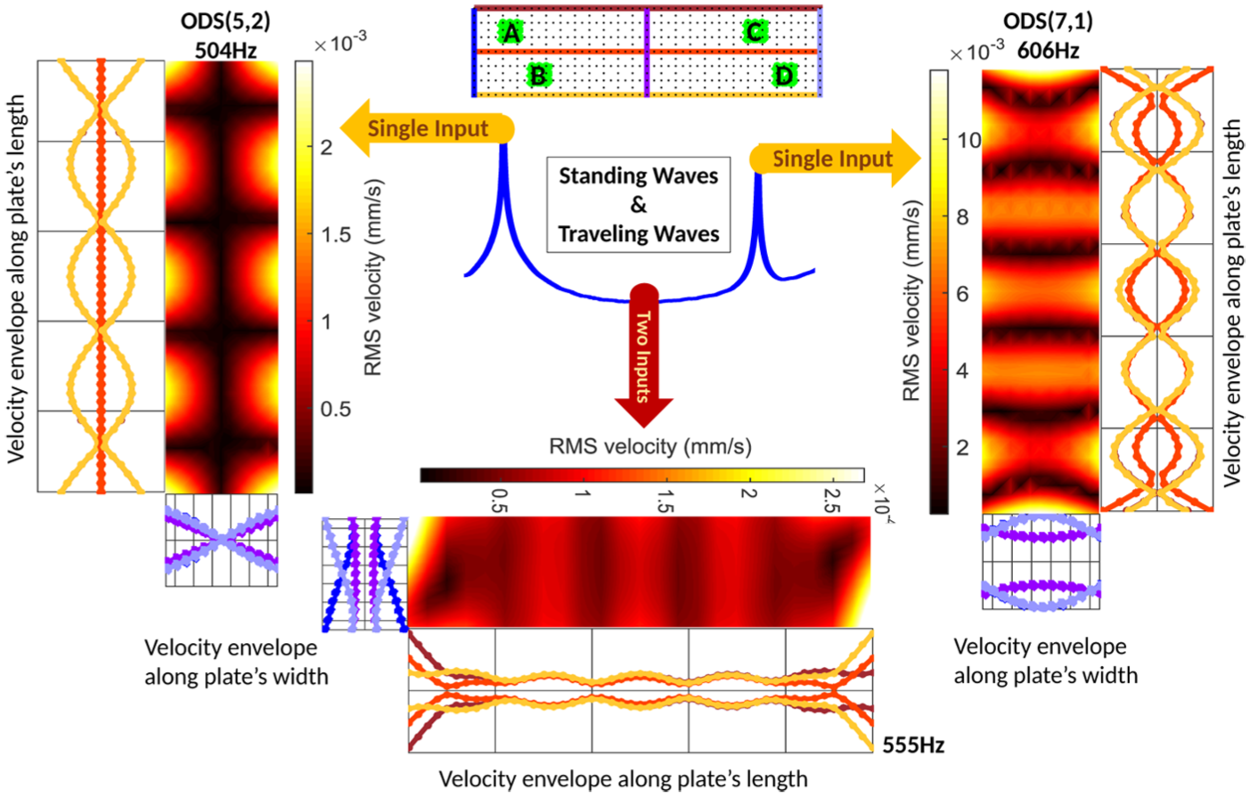
RMS contour plot and wave envelope plot for standing and traveling waves.
For example, either of the single input actuation scenarios shown in this figure have clear nodal lines in the contour plots. Dark regions are parallel to both the length and width of the plate in the case corresponding to the 9th resonant frequency (i.e. ODS(5,2)) and parallel only to the width when the plate is excited at the 10th resonant frequency (i.e. ODS(7,1)). Furthermore, the scenario where the plate is excited by two forces, which are separated by a phase difference of
Additionally, envelope plots along the length and the width of the plate are provided for all cases. Three locations along the length (
Effects of actuation locations
This section discusses the role played by MFC placement in determining the type of resulting 2D planar wave, by changing the actuator pair used to excite the plate. The RMS contour plots in Figure 8 show plate responses when it is excited by three different MFC pairs: A–B, A–C, and A–D. To compare similar plate effects at halfway frequencies, the experimental data at 546 Hz is compared with 555 Hz in simulations for all three scenarios. Contour patterns in all three cases are significantly different from each other, revealing that actuation location plays a significant role when the driving frequency is kept constant. In all three cases, the MFC pairs that are actuated can be easily located in the corners of the plate by identifying areas that are white in color; these areas have particles that have much higher velocities as compared to rest of the plate, as expected. In cases where the plate is excited using the A–B and A–C pairs, there are areas (dark or black in color) where the velocities of the points on the plate are much smaller than the rest of the plate. Although these two scenarios result in complex standing wave patterns, the third case where the plate is excited by the A–D MFC pair, has a recognizable traveling wave pattern. In this case, it is observed that there is a wave that starts at MFC A and travels along the longer side of the plate to reach the other MFC (D). These patterns generated by the FE model closely follow the patterns observed experimentally, which confirms that the excitation locations of the MFCs bonded to the plate play an important role in traveling wave generation. Although, only one of the eight halfway frequencies (294, 374, 448, 546, 635, 708, 805 and 945 Hz) experimentally tested is presented here, a similar trend is observed in most of the cases wherein MFC pairs A–B and A–C generate patterns that are not as good as the wave generated in the A–D pair. Furthermore, in all cases where the plate is excited with the MFC A–D pair (except for 805 Hz), a traveling wave with varying wavelengths is observed. At 805 Hz, a complex standing wave is observed. The experimental RMS contours and wave envelopes for all these cases are plotted along with the averaged frequency response function in Figure 9.
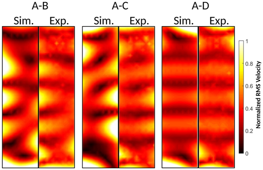
Comparing experimental and simulated RMS velocity contours of the plate at 546 and 555 Hz, respectively.
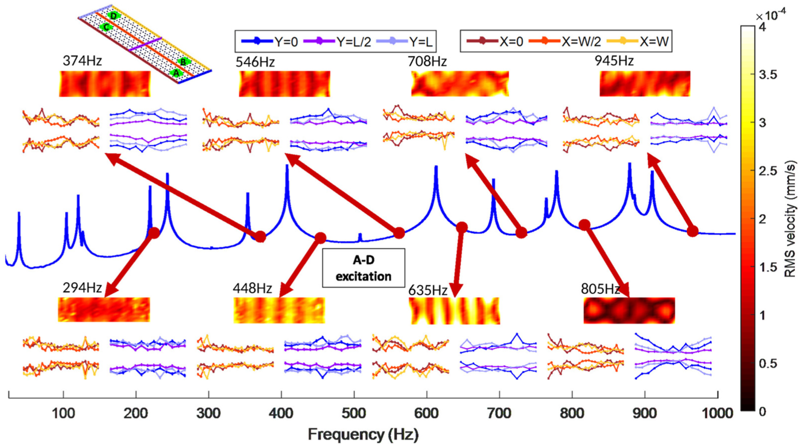
Experimental results for the plate when excited with MFCs A and D.
In the frequency range tested, traveling waves are always found to travel along the length of the plate when the plate is excited using the MFC A–D pair. The direction and the wavelength of these waves vary from case-to-case as shown in Figure 10. In this figure, the time trace contours of the wave progression are presented at four time-stamps: 0,
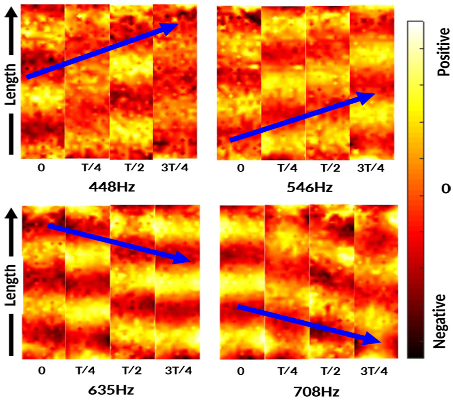
Time frames of wave progression along the length of the plate at times =
Although, as previously stated, most of the experiments with the actuating MFC pair A–B did not result in traveling waves, there is one frequency at which this pair exhibits traveling waves. The experimental plate response at this frequency (635 Hz) is shown in Figure 11. While this wave travels along the length of the plate similarly to the previously discussed results, it also propagates near its long edges and is a combination of waves in both directions. It is easier to visualize this as a traveling wave that is rotating clockwise along the circumference of the plate. As the length of the plate under consideration dominates over its width, this traveling wave appears to be two separate traveling waves progressing in opposite directions. It is quite interesting to note that by changing the location of the forces, at least two different types of traveling wave can exist at a given frequency. This shows the potential to generate multiple traveling waves by changing the location, the frequency of operation and other parameters such as the phase and amplitude.
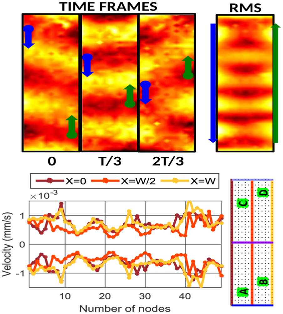
Experimental traveling wave phenomenon in the plate when excited by MFCs A and B at 635 Hz.
Conclusions
Traveling waves studied in the present work are perpetual and steady-state in nature. The goal of the present work is to develop a platform to investigate frequency and location factors that governs the generation of these waves. The research presented in this article focuses on theoretical and experimental investigation of 2D traveling waves in plates. For that purpose, the initial sections of this article discusses the development of a finite element model that govern the dynamics of a rectangular plate bonded with four piezoceramic patches. The numerical results of the FE model are validated through experimental modal tests wherein a rectangular plate is actuated by a single MFC and frequency response characteristics such as mode shapes, natural-frequencies and damping coefficients are estimated. The FE model is updated by evaluating the proportional damping constants through experimental results. This updated model is able to predict up to the 40th damped eigenvalue with a maximum error of 2.5% and match mode shapes accurately, with a lowest MAC value of 0.92.
Once the model is validated, three combinations of MFC pairs are selected and the effect of simultaneous actuation of multiple piezos on the plate is studied. The experimental and simulated responses of the plate at halfway frequencies, are compared for all three scenarios. The response patterns in all three cases are significantly different from each other, revealing that actuation location plays a significant role when the driving frequency is kept constant. For example, when the plate is excited at 555 Hz using the A–B and A–C pairs, the plate results in complex standing wave patterns. However, 2D traveling waves are successfully developed in the plate when it is simultaneously excited by the A–D MFC pair. In the frequency range tested, traveling waves are always found to travel along the length of the plate when the plate is excited using the MFC A–D pair. Our investigation suggests that the wavelength and the type of traveling waves can be varied by changing the frequency of excitation. Several factors affecting the quality of traveling waves, such as frequency and excitation location, are investigated in the present work.
The results presented show that at some frequencies, the type of traveling wave can also be changed by varying the location of the actuator. However, to fully understand the dynamics of this phenomenon, a quantitative measure that describes the quality of the wave is to be established. There are cost–function formulations based on 2D-fft analysis to quantify the quality of a wave. These techniques are an extension of the well-established 1D wave identification methods based on Fourier transform, Hilbert transform, etc. A similar approach will be undertaken in future, to understand the effects of phase difference between the two voltage signals, the location of the piezoceramics, and the number of piezoceramics on the resulting traveling wave. The results shown in this article pave the way to understand the full potential of traveling waves in plates. This work is a step towards integrating the dynamics of biological systems into engineering systems. Steady-state traveling waves in a 2D structure directly impact the development of bio-inspired vehicles with better aerodynamics, and bio-mimicking robotics.
Footnotes
Appendix 1
Elements of the reduced stiffness matrix, appearing in equation (5) as a function of Young’s modulus of elasticity, E, and Poisson’s ratio,
For a piezoelectric actuator operating in 1-3 mode
Appendix 2
Declaration of Conflicting Interests
The author(s) declared no potential conflicts of interest with respect to the research, authorship, and/or publication of this article.
Funding
The author(s) disclosed receipt of the following financial support for the research, authorship, and/or publication of this article: The authors would like to acknowledge the support of the Air Force Office of Scientific Research through the Young Investigator Program (FA9550-15-1-0198).