Parametric investigation of twin tube magnetorheological dampers using a new unsteady theoretical analysis

Abstract

In the present work, a new unsteady analytical model is developed for magnetorheological fluid flow through the annular gap which is opened on the piston head of twin tube magnetorheological damper, considering fluid inertia term into the momentum equation. This new unsteady model is based on Stokes’ second problem that is extended for magnetorheological fluid flow between finite oscillating parallel plates under the pressure gradient. A quasi-static analysis is also developed for magnetorheological fluid flow in twin tube damper, to compare its results with present unsteady solution and to show the effect of magnetorheological fluid inertia. The obtained results are validated experimentally and then, a parametric study is presented using both unsteady and quasi-static analysis. The effect of fluid inertia term is investigated on force–displacement and force–velocity loops, magnetorheological fluid velocity profile, pressure drop, phase difference between pressure drop and flow rate and change of plug thickness with time duration. According to the obtained results, quasi-static analysis included considerable error respect to new unsteady analysis as the gap height, magnetorheological fluid density, excitation frequencies and amplitudes are increased and yield stress is decreased. It is found that the plug thickness is considerably affected by inertia term of magnetorheological fluid.

Keywords

Magnetorheological fluid flow magnetorheological damper fluid inertia unsteady flow damping force plug thickness

1. Introduction

Magnetorheological fluid (MRF) and electrorheological fluid (ERF) are smart fluids that display a reversible and rapid transition behavior from a free flowing state to a semi-solid state in the presence of external magnetic and electric field. The yield stress of smart fluids can be changed and controlled by tuning the intensity of the applied field. One of the most important applications of magnetorheological fluid (MRF) and electrorheological fluid (ERF) are magnetorheological (MR) and electrorheological (ER) dampers which are employed in vibration control of vehicles and building structures.

In the past decades, many studies have been conducted for MRF and MR damper modeling. Experimental, computational fluid dynamics (CFD), and analytical modeling of MR dampers have been presented by several researchers (Parlak and Engin, 2012; Soda et al., 2001; Sternberg et al., 2014; Wereley and Pang, 1998). Analytical model can be used instead of more complex and expensive CFD or experimental models. In analytical models, Navier–Stokes equations are solved analytically for MRF and ERF flow. A non-dimensional analysis was investigated by Phillips (1969), where a set of non-dimensional variables and a corresponding polynomial solution was developed to determine the pressure gradient of the flow through a parallel duct based on quasi-static analysis. Bingham plastic and biplastic force responses to constant velocity input were compared by Dimock et al. (2002), using quasi-static analysis. A quasi-static axisymmetric model of MR dampers was derived and then compared with both a simple analytical parallel plate model and experimental results by Yang et al. (2002). They found that these models are not sufficient to describe the dynamic behavior of MR dampers and a mechanical model based on the Bouc–Wen hysteresis model was developed by them. Four non-dimensional design parameters based on the Bingham plastic constitutive equation of the MRF were defined by Hong et al. (2005). They investigated the design characteristics of each parameter and then formulated sequential design steps for the MR damper. An axisymmetric quasi-steady Bingham plastic model for an MR flow mode damper was analyzed by Yoo and Wereley (2005). They approximated equivalent viscous damping coefficient (C_eq/C) for the annular duct which was equivalent with the one for the rectangular duct when the small gap assumption was applied. Ai et al. (2006) developed a mathematical model for the MR valve with both annular and radial flow paths based on quasi-static assumption. According to their results, the efficiency of the MR valve with circular disk-type fluid resistance channels is superior to that with annular fluid resistance channels under the same magnetic flux density and outer radius of the valve. Brigley et al. (2007) presented an experimental and theoretical evaluation of novel type of multi-mode MR isolator against multi-degree-of-freedom excitations. For theoretical model of the MR isolator, its dynamic equation was derived and important model parameters was identified by the force averaging method. A parametric study of a MR valve and a MR orifice was investigated by Grunwald and Olabi (2008) based on quasi-study assumption. According to their results, achievable pressure drop for the valve layout was significantly higher than those for the orifice layout. A quasi-study analytical non-dimensional Bingham model for mixed-mode MR damper was described by Hong et al. (2008). They analyzed the effects of the Bingham number and the hydraulic amplification ratio on the non-dimensional plug thickness and equivalent viscous damping coefficient. Wang et al. (2009) analytically and experimentally compared the performances of a MR valve with both annular and radial fluid flow resistance gaps with those of the MR valve with only annular fluid flow gaps. According to their results, the pressure drops across the MR valve with both annular and radial fluid flow gaps are larger than those across the MR valve with only annular fluid flow gaps for varying valve parameters. Due to the yield behavior of MRFs, viscoplastic rheological models are usually used to describe the behavior of MRFs (Ghaffari et al., 2014). One of the most convenient rheological models for ERF and MRF is Bingham plastic model (Kamath et al., 1996; Yoo and Wereley, 2005), which is used in present new unsteady analytical model. The quasi-static analysis for the MRF flow in the annular duct was evaluated by Khan et al. (2014). They mathematically modeled the MR damper based on Bingham plastic model and Herschel–Bulkley model. Usually, analytical solutions and all design formulas are based on quasi-static steady assumption (Ai et al., 2006; Brigley et al., 2007; Dimock et al., 2002; Ghaffari et al., 2014; Grunwald and Olabi, 2008; Hong et al., 2005, 2008; Kamath et al., 1996; Khan et al., 2014; Parlak and Engin, 2012; Phillips, 1969; Wang et al., 2009; Yang et al., 2002; Yoo and Wereley, 2005a, 2005b). This assumption is suitable under steady-state conditions and very low range of the oscillatory frequency.

Despite considerable effect of fluid inertia and unsteady behavior of MRF flow, it is ignored in most of previous studies. Therefore, it is important to study unsteady-state conditions of MRF flow within MR damper to describe its actual operation. Chen et al. (2004) solved pressure gradient and velocity profile of the unsteady-state unidirectional flow of Bingham fluid between parallel plates using the Laplace transform method. No diagram was plotted in their paper to validate and evaluate the results of their method. A new method for dynamic modeling of an ER damper was proposed by Nguyen and Choi (2009), considering the unsteady behaviors of ERF flow through the annular duct. According to their results, the effect of unsteady behavior should be taken into account at high frequencies. In their study, the implemented equilibrium equation was based on quasi-static assumption which seems a wrong assumption for an unsteady analysis. Yu et al. (2013) theoretically analyzed unsteady flow of MRFs within flow mode MR dampers (with valve parallel to cylinder and fix walls), by means of numerical velocity solutions of partial differential equation (PDE) and variable separation method. The Newtonian regions, in parallel to the coil, are not considered in their calculations for damping force.

The purpose of the present study is to introduce a novel unsteady analytical model, based on Stokes’ second problem (Stokes, 1851), for MRF flow through the annular gap which is opened on the piston head of twin tube MR damper, considering fluid inertia term into the momentum equation. Here, governing equation for MRF flow in annular gap inside the moving piston of MR damper is solved based on the extending Stokes’ second problem for non-Newtonian (MR) and Newtonian fluid flow through oscillating parallel plates under the periodic pressure gradient. Using this method, velocity profile is predicted for different flow regions. Then pressure gradient and also inner and outer boundaries of plug region within the gap is obtained by solving nonlinear systems of equations. A quasi-static analysis is also developed for MRF flow in annular gap inside the moving piston head, to compare its results with present unsteady analysis results. The unsteady and quasi-static analysis results are validated by comparing them against experimental data. Then, under different excitation frequencies and amplitudes, yield stresses, densities and gap heights, operation of MR damper are investigated in detail.

2. Problem statement

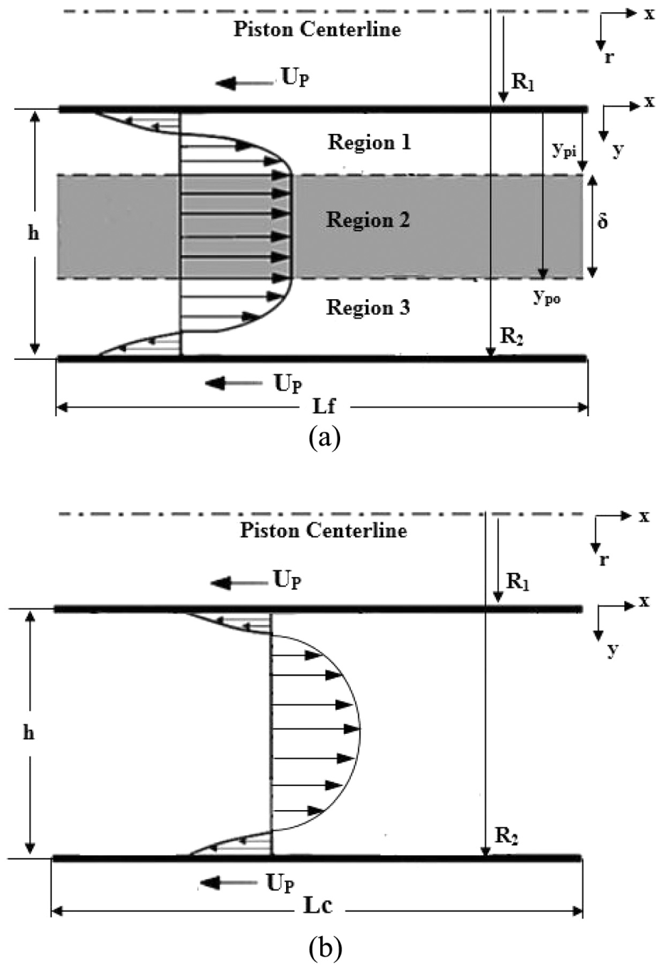
A schematic view of a twin tube MR damper is shown in Figure 1. Due to the motion of piston, the oil flows through the annular gap inside the piston. Regions within the gap in parallel to coil are not magnetized (are not affected by magnetic field) and the fluid in these regions could be considered Newtonian while the regions within the gap in parallel to flange are magnetized so the fluid in these regions is non-Newtonian (Bingham plastic). The ratio of gap to piston diameter is small, so the flow through the gap can be considered as the two-dimensional flow between parallel plates which is shown in Figure 2. This approximation is seen to be adequate for practical design and commonly is used to approximate ER/MR behavior in annular geometries (Burton et al., 1996; Gavin, 1998; Jolly et al., 1999; Kamath et al., 1996; Wereley and Pang, 1998; Yang et al., 2002). In this study, an unsteady analytical model is proposed based on solving the momentum equations and extending Stokes’ second problem (Stokes, 1851) for non-Newtonian (MR) and Newtonian fluids flow between oscillating parallel plates with finite depth under the periodic pressure gradient.

Figure 1.

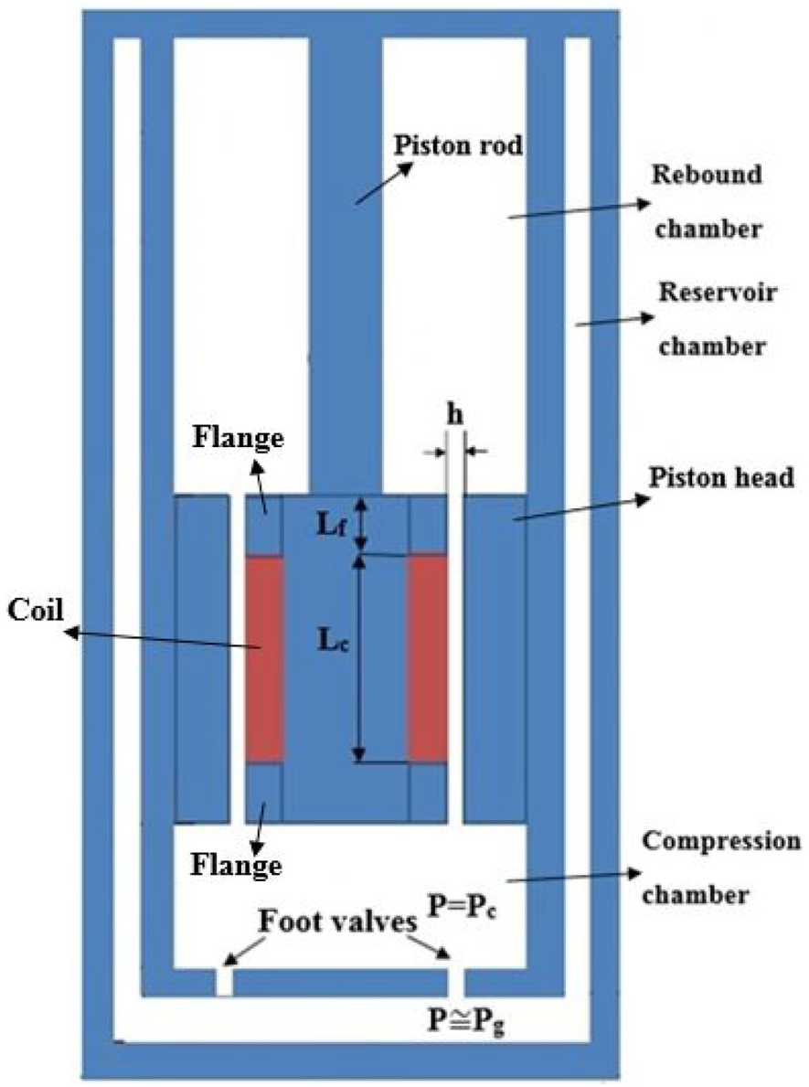
Schematic view of twin tube MR damper.

Figure 2.

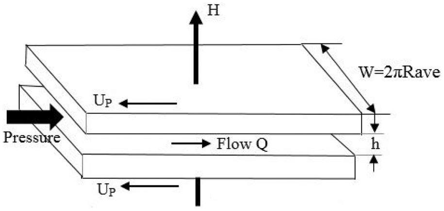
Schematic view of approximated parallel plate model of gap inside the piston.

3. Governing equations and constitutive equation

The governing equations consist of the continuity and momentum equations for incompressible flows

\nabla \cdot U = 0

(1)

ρ \frac{DU}{Dt} = - \nabla P + \nabla \cdot τ

(2)

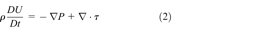
where t is time, U is velocity vector, ρ is density, $\nabla P$ is pressure gradient, and τ is shear stress.

Here, Bingham plastic model is employed to describe the non-Newtonian behaviors of the MRF. In this model, shear stress is given as follows (Kamath et al., 1996; Yoo and Wereley, 2005)

τ = τ_{y} (H) sign (\overset{\cdot}{γ}) + μ \overset{\cdot}{γ} | τ | > τ_{y}

(3)

\overset{\cdot}{γ} = 0 | τ | \leq τ_{y}

(4)

where τ is the shear stress, τ_y is the yield stress due to the applied magnetic field, $H$ is the amplitude of applied magnetic field, $μ$ is the viscosity of MRFs, and $\overset{\cdot}{γ}$ is the shear strain rate. Substituting equation (3) into equation (2), τ_y is eliminated. It is important to remember that τ_y is a property of fluid that is a property of fluid that is just depended on H (independent from directions). Due to the very small size of the gap, the flow is also laminar and fully developed and because of the domination of viscous force, the effect of gravitational acceleration is negligible. Therefore, the following relation for post-yielded regions ( $| τ | > τ_{y}$ ) is obtained

ρ \frac{\partial U}{\partial t} = - \frac{d P}{d x} + μ \frac{\partial^{2} U}{\partial y^{2}}

(5)

In the axisymmetric model, the yield stress τ_y is related to r due to the radial distribution of the magnetic field in the gap. However, if $h < < R_{ave}$ or R₂, then axisymmetric geometry can be approximated by parallel plate geometry and the variation of the yield stress in the gap can be ignored (Bird et al., 1960; Gavin, 2001; Phillips, 1969; Yang et al., 2002). In present work, the maximum investigated gap height is h = 0.0015, and corresponding outer radius of the gap is R₂ = 0.0109, so h/R₂ = 0.15, and maximum error between two models is not more than 0.5% (Yang et al., 2002). It is important to mention that the effect of yield stress appears in boundary conditions and velocity profile that will be explained in the next section.

4. Unsteady analysis

4.1. Determining the velocity field

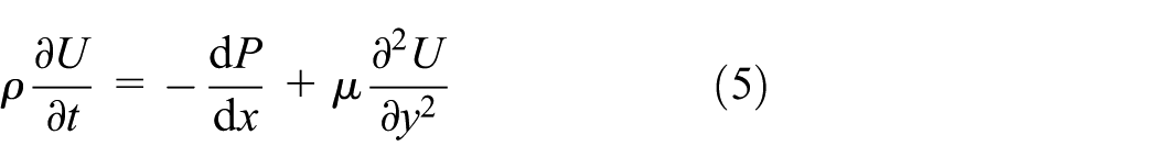
Due to the fluid flow inside the moving piston, a non-inertial coordinates system which is moving with the accelerating system can be used (White, 2006). Here, it is assumed that the non-inertial coordinates system is attached to the piston. Therefore, the absolute acceleration, $a_{abs}$ , and absolute velocity of a particle, U_abs, can be related to their relative values as follows

U_{abs} = - U_{p} + U_{rel}

(6)

a_{abs} = - a_{p} + a_{rel}

(7)

Substituting equations (6) and (7) into equation (2) gives

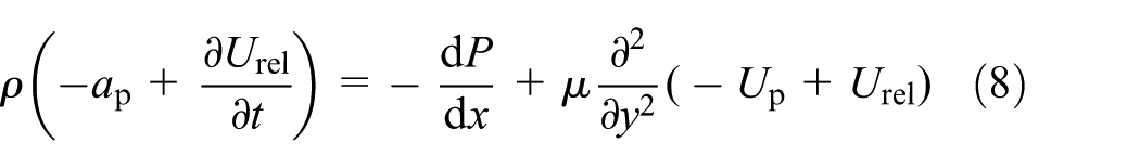
ρ (- a_{p} + \frac{\partial U_{rel}}{\partial t}) = - \frac{d P}{d x} + μ \frac{\partial^{2}}{\partial y^{2}} (- U_{p} + U_{rel})

(8)

Flow field can be approximated as flow through two oscillating parallel plates that is shown in Figure 2. The analytical solution of governing equations is too complex for unsteady flows. Using the present method, PDE is simplified to ordinary differential equations (ODEs) which reduces the difficulties of solving the original PDE. Here, based on Stokes’ second problem (Stokes, 1851), for a long-time steady oscillation, the transient or start-up of the flow can be neglected (White, 2006) and the steady oscillatory solution of equation (8) can be expressed in the form of equation (9). The pressure gradient is also defined as equation (10), so that the argument of complex value of K is related to the phase difference between velocity and pressure gradient. Velocity and acceleration of piston can be shown in equations (11) and (12), respectively. In these equations, $ω = 2 π f$ in which f and A are oscillation frequency and amplitude, respectively

U_{rel} (y, t) = {\bar{U}}_{rel} (y) \exp (i ω t)

(9)

\frac{d p}{d x} = - ρ K \exp (i ω t)

(10)

U_{p} = A ω \exp (i ω t)

(11)

a_{p} = A i ω^{2} \exp (i ω t)

(12)

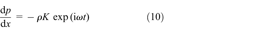
Substituting equations (9) to (12) into equation (8) gives the following ordinary differential equation

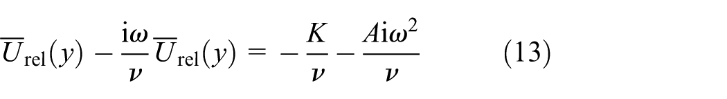
{\bar{U}}_{rel} (y) - \frac{i ω}{ν} {\bar{U}}_{rel} (y) = - \frac{K}{ν} - \frac{A i ω^{2}}{ν}

(13)

By solving equation (13), the relative and absolute velocity is obtained as

\begin{matrix} U_{rel} (y, t) = & {C_{1} \exp (\sqrt{\frac{i ω}{υ}} \cdot y) + C_{2} \exp (- \sqrt{\frac{i ω}{υ}} \cdot y) \\ + \frac{K}{i ω} + A ω} \exp (i ω t) \end{matrix}

(14)

\begin{matrix} U_{abs} (y, t) = & {C_{1} \exp (\sqrt{\frac{i ω}{υ}} \cdot y) + C_{2} \exp (- \sqrt{\frac{i ω}{υ}} \cdot y) \\ + \frac{K}{i ω}} \exp (i ω t) \end{matrix}

(15)

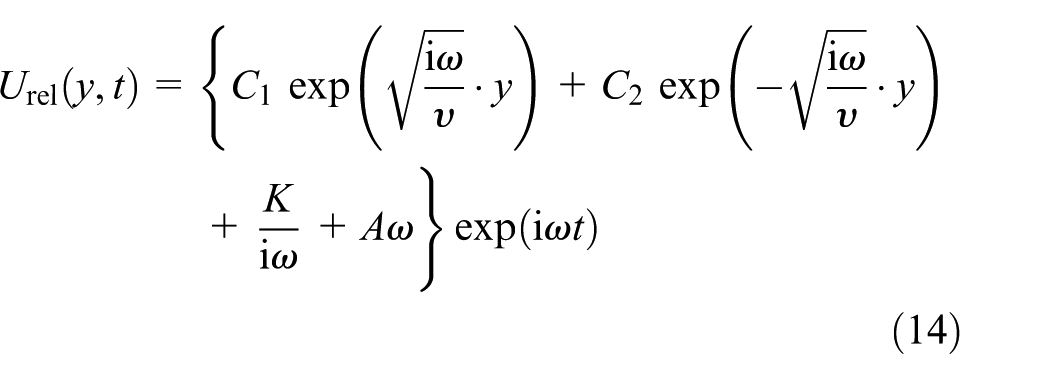
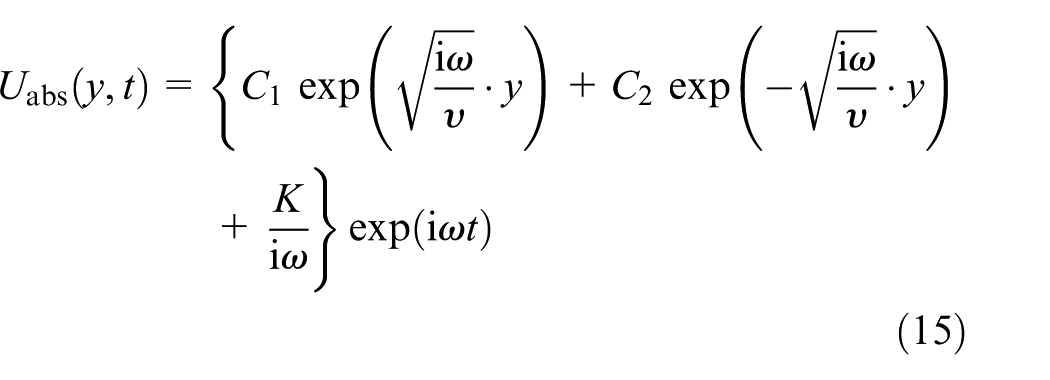
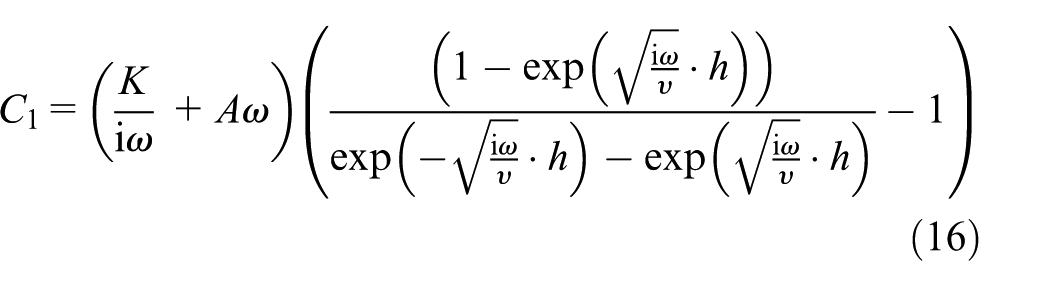
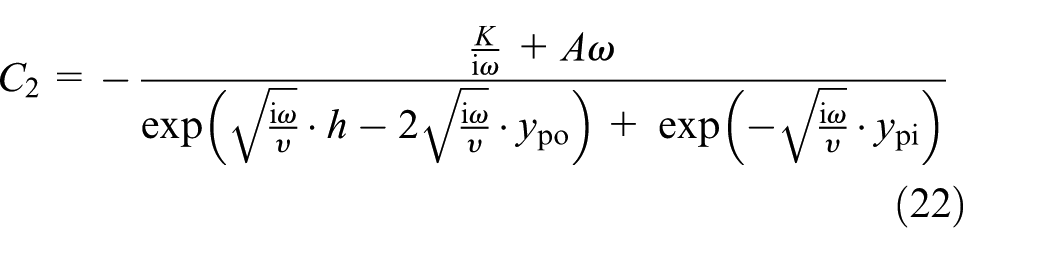
Due to considering the constant values for yield stress and viscosity, the Navier–Stokes equations for the Newtonian region is the same as the one for the post-yielded region of MRF (equation (8)). Therefore, the overall form of the obtained velocity profile (equation (15)) is the same for both regions; butte constants of velocity profile of each region are different and are obtained from the corresponding boundary conditions that are given in Table 1. A schematic view of the velocity profile and boundary conditions of non-Newtonian flow region in gap is shown in Figure 3(a). In this figure, regions 1 and 3 are the post-yield regions, where the shear stress exceeds the yield stress and the fluid flows, and region 2 is plug flow region, where the shear stress is less than the yield stress and velocity is constant across this region. Here, y_pi and y_po are inner and outer boundaries of plug flow region. A schematic view of the velocity profile of Newtonian flow region is also shown in Figure 3(b). Applying the given boundary conditions presented in Table 1, C₁ and C₂ are obtained for fluid velocity profile of each region which are expressed in following sections.

Table 1.

Boundary conditions in each region.

Region	y = 0	y = y_pi	y = y_po	y = h
Newtonian flow	$U_{rel} = 0$			$U_{rel} = 0$
Non-Newtonian (MR) flow	$U_{rel} = 0$	$\partial (U_{rel}) / \partial y = 0$	$\partial (U_{rel}) / \partial y = 0$	$U_{rel} = 0$

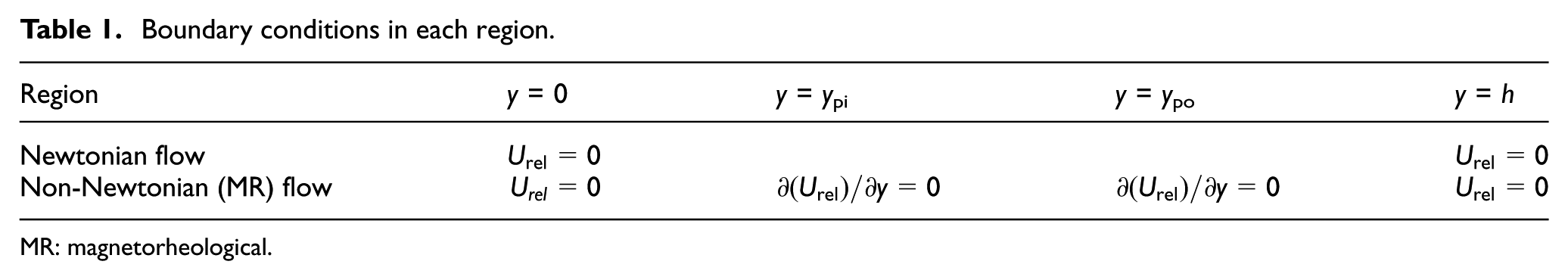
MR: magnetorheological.

Figure 3.

Schematic view of absolute velocity profile and boundary conditions for (a) non-Newtonian (MR) regions and (b) Newtonian regions.

4.1.1. Newtonian regions

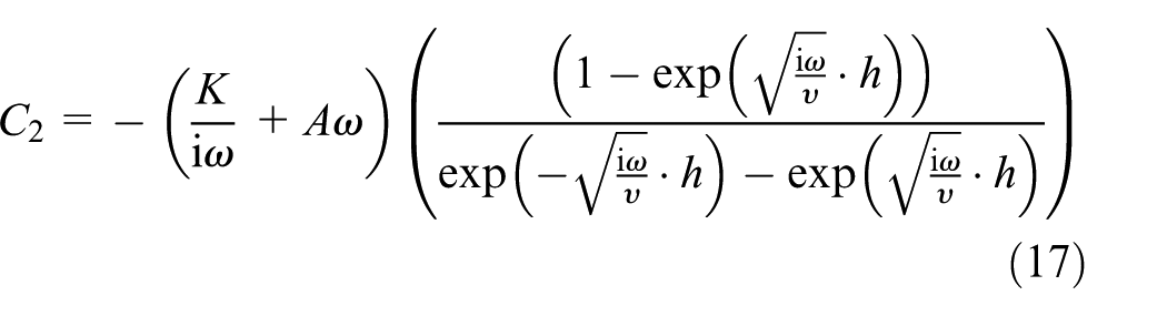
Regions within the gap in parallel to the coil are not magnetized and the fluid in these regions is Newtonian. Two constants of C₁ and C₂ are obtained for fluid velocity profile of these regions as follows

C_{1} = (\frac{K}{i ω} + A ω) (\frac{(1 - \exp (\sqrt{\frac{i ω}{υ}} \cdot h))}{\exp (- \sqrt{\frac{i ω}{υ}} \cdot h) - \exp (\sqrt{\frac{i ω}{υ}} \cdot h)} - 1)

(16)

C_{2} = - (\frac{K}{i ω} + A ω) (\frac{(1 - \exp (\sqrt{\frac{i ω}{υ}} \cdot h))}{\exp (- \sqrt{\frac{i ω}{υ}} \cdot h) - \exp (\sqrt{\frac{i ω}{υ}} \cdot h)})

(17)

4.1.2. Non-Newtonian (MR) regions

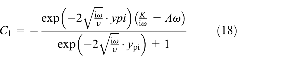
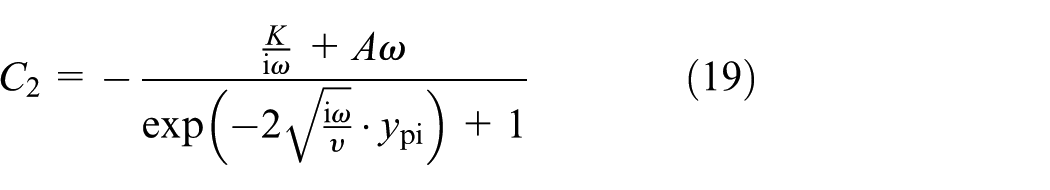
The regions within the gap in parallel to flange are magnetized so the fluid in these regions is non-Newtonian (Bingham plastic). As shown in Figure 3(a), this region is divided into post-yield regions (regions 1 and 3) and plug region (region 2). Applying the given boundary conditions which are introduced in Table 1, C₁ and C₂ are obtained for fluid velocity profile of each region as follows:

Region 1

C_{1} = - \frac{\exp (- 2 \sqrt{\frac{i ω}{υ}} \cdot ypi) (\frac{K}{i ω} + A ω)}{\exp (- 2 \sqrt{\frac{i ω}{υ}} \cdot y_{pi}) + 1}

(18)

C_{2} = - \frac{\frac{K}{i ω} + A ω}{\exp (- 2 \sqrt{\frac{i ω}{υ}} \cdot y_{pi}) + 1}

(19)

Region 2

Because the velocity is constant across the plug region, so

U_{abs 2} (y, t) = U_{rel 1} (y_{pi}, t) = U_{abs 3} (y_{po}, t)

(20)

C ₁ and C₂ for the velocity profile in this region are the same as the one for region 1 or region 2.

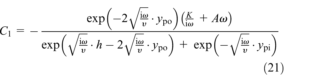
Region 3

C_{1} = - \frac{\exp (- 2 \sqrt{\frac{i ω}{υ}} \cdot y_{po}) (\frac{K}{i ω} + A ω)}{\exp (\sqrt{\frac{i ω}{υ}} \cdot h - 2 \sqrt{\frac{i ω}{υ}} \cdot y_{po}) + \exp (- \sqrt{\frac{i ω}{υ}} \cdot y_{pi})}

(21)

C_{2} = - \frac{\frac{K}{i ω} + A ω}{\exp (\sqrt{\frac{i ω}{υ}} \cdot h - 2 \sqrt{\frac{i ω}{υ}} \cdot y_{po}) + \exp (- \sqrt{\frac{i ω}{υ}} \cdot y_{pi})}

(22)

4.2. Obtaining pressure drop in Newtonian regions

We need an additional equation to obtain the pressure drop in Newtonian regions (in parallel to the coil). The additional equation can be obtained based on the equality of the flow rate through the gap, Q_g, with the volume flow rate which is displaced by the piston head, Q_p

Q_{g} = U_{P} (A_{P} - A_{r})

(23)

2 π R_{ave} (\int_{0}^{h} U_{abs} (y, t) d y) = A ω \exp (i ω t) (A_{P} - A_{r})

(24)

where $A_{P}$ and $A_{r}$ are the cross sections of piston area and rode area, respectively. Also, absolute velocity, U_abs(y, t), is obtained from equations (15) to (17) and includes unknown K. It is a complex variable which is obtained from equation (25) and its imaginary part is related to the phase difference between velocity and pressure gradient ( $ϕ$ ) (Kreyszig, 1983). Therefore, the term K can be determined as follows

K = | K | \exp (i ϕ)

(25)

ϕ = \tan^{- 1} (\frac{Imaginary of K}{Real of K})

(26)

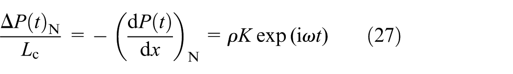
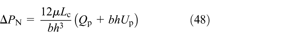
Then, pressure gradient dP(t)/dx)_N and pressure drop ΔP(t)_N in Newtonian regions can be determined using the obtained K and equation (27) as follows

\frac{Δ P {(t)}_{N}}{L_{c}} = - {(\frac{d P (t)}{d x})}_{N} = ρ K \exp (i ω t)

(27)

4.3. Obtaining pressure drop, y_pi and y_po, in non-Newtonian (MR) regions

For non-Newtonian regions (in parallel to flanges), three coupled nonlinear equations should be solved numerically to determine three unknown of K, y_pi, and y_po. Then, pressure gradient (dP(t)/dx)_MR can be determined using the obtained K. The three nonlinear equations with three unknown of K, y_pi, and y_po are continuity equation, continuity of velocity profile at boundaries of plug region, and force equilibrium for plug region, which are introduced in following sections.

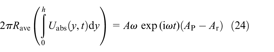
4.3.1. Continuity equation

The total volume flow rate through the gap, $Q_{g}$ , in non-Newtonian (MR) regions must be equal to the volume flow rate displaced by the piston head, Q_p

Q_{g} = Q_{1} + Q_{2} + Q_{3} = U_{P} (A_{P} - A_{r})

which leads to

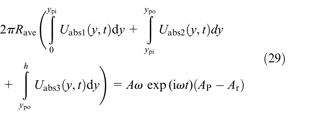
\begin{matrix} 2 π R_{ave} (\int_{0}^{y_{pi}} U_{abs 1} (y, t) d y + \int_{y_{pi}}^{y_{po}} U_{abs 2} (y, t) dy \\ + \int_{y_{po}}^{h} U_{abs 3} (y, t) d y) = A ω \exp (i ω t) (A_{P} - A_{r}) \end{matrix}

(29)

where U_abs1(y, t), U_abs2(y, t), and U_abs3(y, t) can be substituted from equations (15) to (22).

4.3.2. Continuity of velocity profile at boundaries of plug region

The velocity of MRF flow at the boundaries of the plug region (region 2) should be equal due to the fact that the velocity is constant across the plug region, so

U_{abs 2} (y_{pi}, t) = U_{abs 3} (y_{po}, t)

(30)

Equation (30) includes three unknowns of K, y_pi, and y_po.

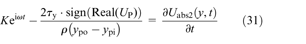
4.3.3. Force equilibrium for plug region

As shown in Figure 4, MRF enclosed in plug region between y = y_pi and y = y_po (region 2). Force equilibrium for this region leads to

K e^{i ω t} - \frac{2 τ_{y} \cdot sign (Real (U_{P}))}{ρ (y_{po} - y_{pi})} = \frac{\partial U_{abs 2} (y, t)}{\partial t}

(31)

Figure 4.

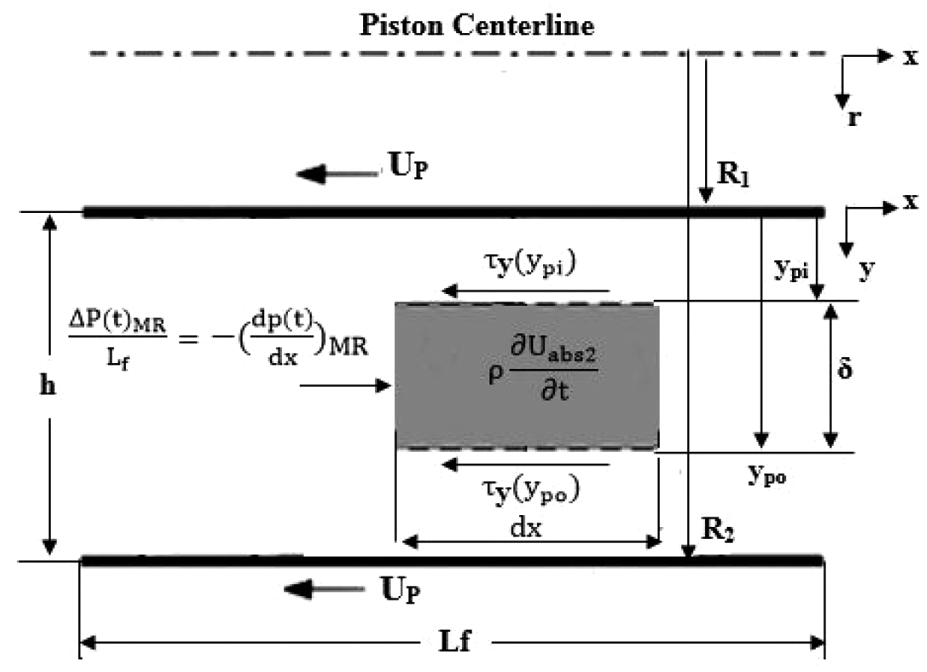
Force equilibrium of plug region (region 2).

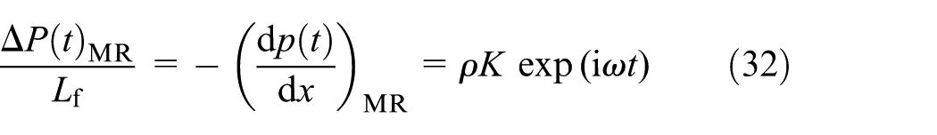
The system of three nonlinear equations (29) to (31) with three unknowns is solved numerically and K, y_pi, and y_po are obtained. Then pressure gradient and pressure drop in MR regions can be determined from equation (32)

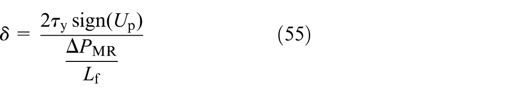
\frac{Δ P {(t)}_{MR}}{L_{f}} = - {(\frac{d p (t)}{d x})}_{MR} = ρ K \exp (i ω t)

(32)

Also, the plug thickness δ(t) can be obtained from resultant plug boundaries, y_pi and y_po, in each time as follows

δ (t) = y_{po} - y_{pi}

(33)

On the other hand, considering equation (32) and rewriting equation (31) yield the following relation for the plug thickness

δ (t) = \frac{2 τ_{y} \cdot sign (Real (U_{P}))}{\frac{Δ P {(t)}_{MR}}{L_{f}} - ρ \frac{\partial U_{abs 2} (y, t)}{\partial t}}

(34)

4.4. Damping force

As there are two MR regions in parallel to flanges and one Newtonian region parallel to the coil in annular gap of piston, the total pressure drop can be obtained from equation (35)

Δ P {(t)}_{total} = Δ P {(t)}_{MR} \times 2 L_{f} + Δ P {(t)}_{N} \times L_{c}

(35)

where ΔP(t)_N and ΔP(t)_MR can be determined from equations (27) and (32). Then, damping force can be obtained as

\begin{matrix} F_{d} (t) = & - (Δ P {(t)}_{total} (A_{P} - A_{r}) + P_{c} (A_{r}) \\ + sign (Real (U_{P})) F_{s} \end{matrix}

(36)

where P_c is pressure of compression chamber and according to Figure 1, can be determined in compression and rebound as follows

P_{c, Compression} = P_{g} + Δ P_{valve}

(37)

P_{c, Rebound} = P_{g} - Δ P_{valve}

(38)

Assuming that the volume of gas V_g in the reservoir chamber satisfies the equation of polytropic processes (Ferdek and Luczko, 2012), the pressure of the gas P_g in each time can be obtained from

P_{g} = P_{0} {(\frac{V_{0}}{V_{g}})}^{n}

(39)

where n is the coefficient of the polytropic and is assumed to be n = 1.4 (Ferdek and Luczko, 2012). V₀ and P₀ are initial volume and pressure in the reservoir chamber. Also, V_g in each time can be determined as

V_{g} = V_{0} + A_{r} X_{P} (t)

(40)

where X_p(t) is piston displacement and is assumed to be a sinusoidal excitation as follows

X_{P} (t) = A ω \sin (ω t)

(41)

Pressure difference of the foot valves, $Δ P_{valve}$ can be obtained from frequent algebraic models of valve in the shock absorber handbooks (Dixon, 2007)

Δ P_{valve} = \frac{1}{2} ρ {(\frac{Q_{valve}}{C_{d} A_{valve}})}^{2}

(42)

where estimated values of the discharge coefficient C_d are likely to be around 0.7, practically (Dixon, 2007). A_valve is effective area of the valves and Q_valve is the flow rate in valves that can be determined as

Q_{valve} = A_{r} {\overset{\cdot}{X}}_{P} (t)

(43)

Also, $F_{s}$ in equation (36) is the Coulomb friction force and should be measured experimentally.

5. Quasi-static analysis

The quasi-static analysis is usually used to design the MR dampers. Convectional design formulas (Nguyen and Choi, 2009) and analyses (Wereley and Pang, 1998) for approximate rectangular parallel plate model of the valve mode MR damper were presented for a valve with fixed walls. When the annular gap is located inside the moving piston, the motion of the wall should be taken into account as boundary conditions. In this study, a quasi-static analysis is developed for approximate rectangular parallel plate model of the MRF flow in annular gap of moving piston. Considering the velocity of walls, the velocity profile and pressure drop for Newtonian and non-Newtonian regions in the gap are determined as follows.

5.1. Velocity in Newtonian regions

Due to the quasi-static analysis, the inertia term in equation (8) is neglected and direct integration of the outcome results in

U_{rel} (y) = - \frac{Δ P_{N}}{2 μ L_{c}} (y^{2} + C_{1} y + C_{2})

(44)

Applying boundary conditions of Table 1 for Newtonian regions, the velocity of the Newtonian fluid flow in parallel to the coil can be obtained as

U_{rel} (y) = - \frac{Δ P_{N}}{2 μ L_{c}} ((y^{2}) - hy)

(45)

U_{abs} (y) = - \frac{Δ P_{N}}{2 μ L_{c}} ((y^{2}) - hy) - U_{p}

(46)

5.2. Pressure drop in Newtonian regions

Equality of the volume flow rate through the gap with the volume flux displaced by the piston head gives

2 π R_{ave} (\int_{0}^{h} U_{abs} (y) d y) = Q_{p}

(47)

Then, pressure drop can be obtained easily as follows

Δ P_{N} = \frac{12 μ L_{c}}{b h^{3}} (Q_{p} + bh U_{p})

(48)

where b = 2πR_ave, $U_{p} = A ω \cos (ω t)$ , and $Q_{p} = U_{p} (A_{P} - A_{r})$ .

5.3. Velocity in non-Newtonian (MR) region

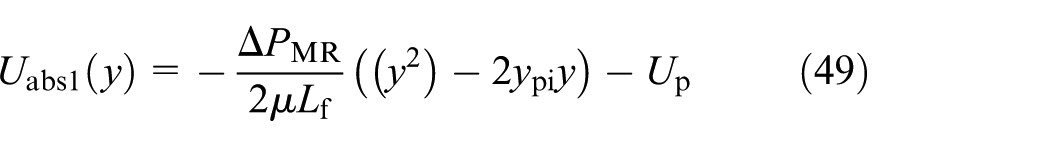
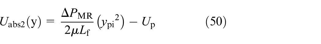
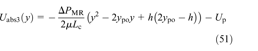
Applying boundary conditions introduced in Table 1 for non-Newtonian (MR) regions, the velocity profile of MRF flow in parallel to flange in the piston gap can be determined as follows

U_{abs 1} (y) = - \frac{Δ P_{MR}}{2 μ L_{f}} ((y^{2}) - 2 y_{pi} y) - U_{p}

(49)

U_{abs 2} (y) = \frac{Δ P_{MR}}{2 μ L_{f}} ({y_{pi}}^{2}) - U_{p}

(50)

U_{abs 3} (y) = - \frac{Δ P_{MR}}{2 μ L_{c}} (y^{2} - 2 y_{po} y + h (2 y_{po} - h)) - U_{p}

(51)

5.4. Pressure drop in non-Newtonian regions

As the velocity is constant across the plug region, the velocity of MRF flow at boundaries of the plug region (region 2) should be equal

U_{abs 1} (y_{pi}) = U_{abs 3} (y_{po})

(52)

which leads to

h = y_{po} + y_{pi}

(53)

On the other hand

δ = y_{po} - y_{pi}

(54)

Also, plug thickness can be obtained from the equilibrium equation of the plug flow as follows

δ = \frac{2 τ_{y} sign (U_{p})}{\frac{Δ P_{MR}}{L_{f}}}

(55)

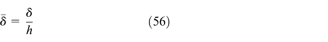
The non-dimensional plug thickness is defined as follows

\bar{δ} = \frac{δ}{h}

(56)

On the other hand, the total volume flow rate through the gap must be equal to volume flow rate which is displaced by the piston head

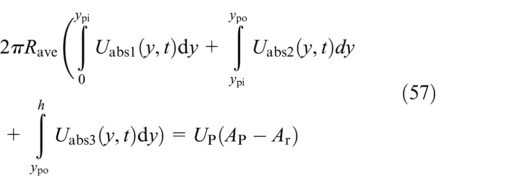
\begin{matrix} 2 π R_{ave} (\int_{0}^{y_{pi}} U_{abs 1} (y, t) d y + \int_{y_{pi}}^{y_{po}} U_{abs 2} (y, t) dy \\ + \int_{y_{po}}^{h} U_{abs 3} (y, t) d y) = U_{P} (A_{P} - A_{r}) \end{matrix}

(57)

Substituting equations (49) to (51) into equation (57), using equations (53) to (56) and direct integration of the outcome leads to

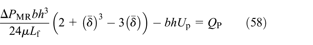
\frac{Δ P_{MR} b h^{3}}{24 μ L_{f}} (2 + {(\bar{δ})}^{3} - 3 (\bar{δ})) - bh U_{p} = Q_{P}

(58)

Substituting equations (55) and (56) into the equation (58) and rewriting the result lead to the following equation for unknown, ΔP(t)_MR

Δ {P_{MR}}^{3} - (C' + 3 B') Δ {P_{MR}}^{2} + 4 B'^{3} = 0

(59)

where

C' = \frac{12 μ L_{f}}{b h^{3}} (Q_{P} + bh U_{p})

(60)

B' = \frac{L_{f} τ_{y} sign (U_{p})}{h}

(61)

By solving equation (59), the pressure drop in MR regions is obtained. Then, damping force from quasi-static analysis can be obtained using the same method that is explained in previous section.

6. Results and discussion

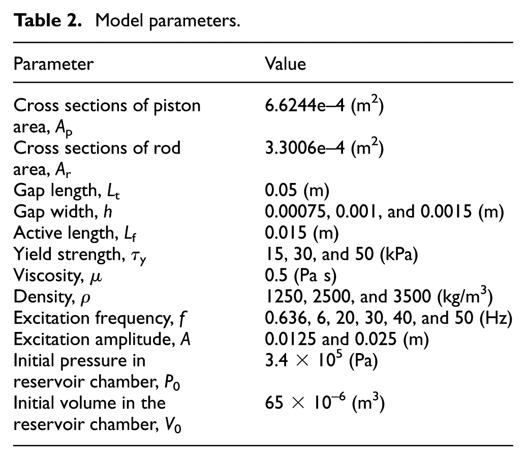
In this section, parametric investigation of twin tube MR dampers with annular gap inside the piston is performed based on a newly proposed unsteady analysis and the results are compared with developed quasi-static analysis. First, the analytical unsteady model is experimentally validated. Therefore, a twin tube MR damper with input current of 4 A is experimentally subjected to sinusoidal excitation with the amplitude of 0.025 m. This load is applied by an Instron dynamic and fatigue testing system (Series 8800, Four-Column Load Frame, single-phase power point, 230 V ± 10% at 50 Hz, maximum range of load cell: 2500 N), which is shown in Figure 5(a). The applied voltage is supplied from a DC voltage source and a current controller is implemented to provide current excitation of the damper coil. The prototype MR damper is shown in Figure 5(b) and its configuration parameters are listed in Table 2.

Figure 5.

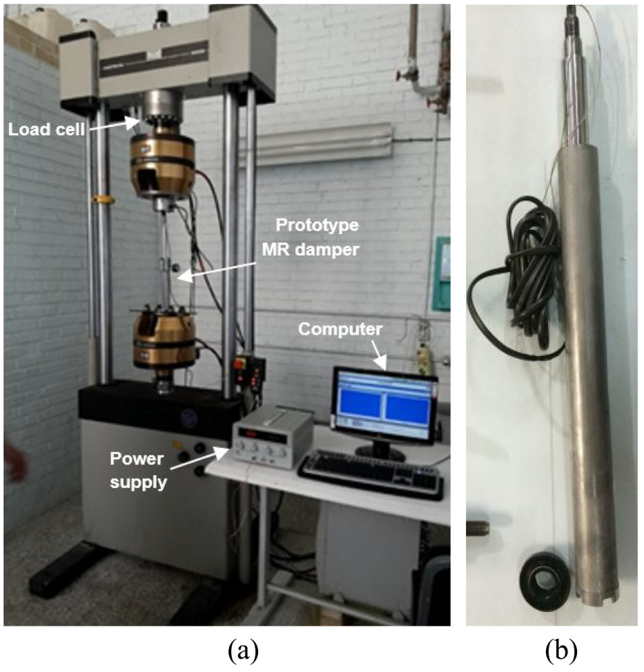
(a) Instron dynamic and fatigue testing system with the damper under test. (b) Prototype MR damper.

Table 2.

Model parameters.

Parameter	Value
Cross sections of piston area, A_p	6.6244e–4 (m²)
Cross sections of rod area, A_r	3.3006e–4 (m²)
Gap length, L_t	0.05 (m)
Gap width, h	0.00075, 0.001, and 0.0015 (m)
Active length, L_f	0.015 (m)
Yield strength, τ_y	15, 30, and 50 (kPa)
Viscosity, µ	0.5 (Pa s)
Density, ρ	1250, 2500, and 3500 (kg/m³)
Excitation frequency, f	0.636, 6, 20, 30, 40, and 50 (Hz)
Excitation amplitude, A	0.0125 and 0.025 (m)
Initial pressure in reservoir chamber, P₀	3.4 × 10⁵ (Pa)
Initial volume in the reservoir chamber, V₀	65 × 10⁻⁶ (m³)

Force–displacement hysteresis loops of MR damper from analytical model and experimental results are compared in Figure 6(a). The mean error between the experimental and analytical results is about 2.2% that may be due to the approximate modeling of the foot valves and polytrophic process assumption in reservoir chamber. Also, a comparison between present method and investigated method by Yu et al. (2013) for double-ended MR damper is shown in Figure 6(b). It is observed that the new unsteady model is in good agreement with the measured values and the results of investigated method by Yu et al. (2013).

Figure 6.

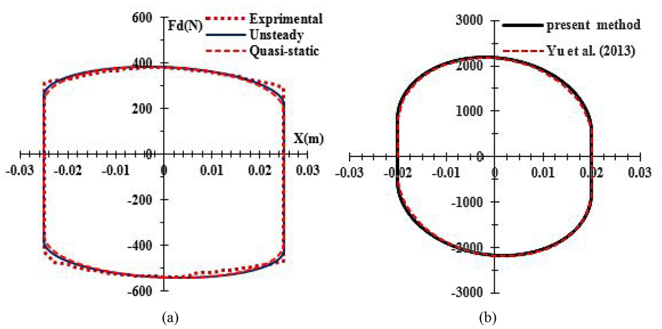
(a) Analytical and experimental force–displacement hysteresis loops for f = 0.636 Hz, ρ = 1250 kg/m³, τ_y = 15 kPa, h = 0.00075 m, A = 0.025 m. (b) Comparison between present method and results reported by Yu et al. (2013) for double-ended MR damper at f = 30 Hz, ρ = 2650 kg/m³&0x44;ÿτ_y = 20 kPa, h = 0.0015 m, A = 0.02 m.

6.1. Effect of frequency

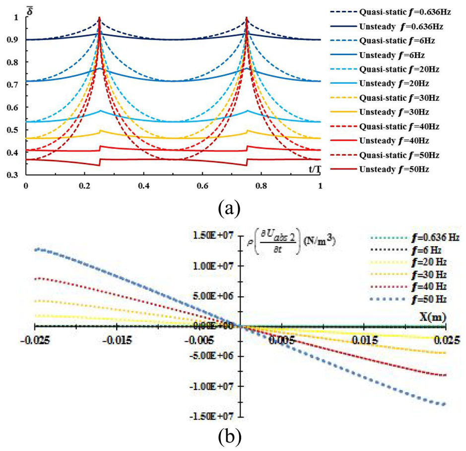
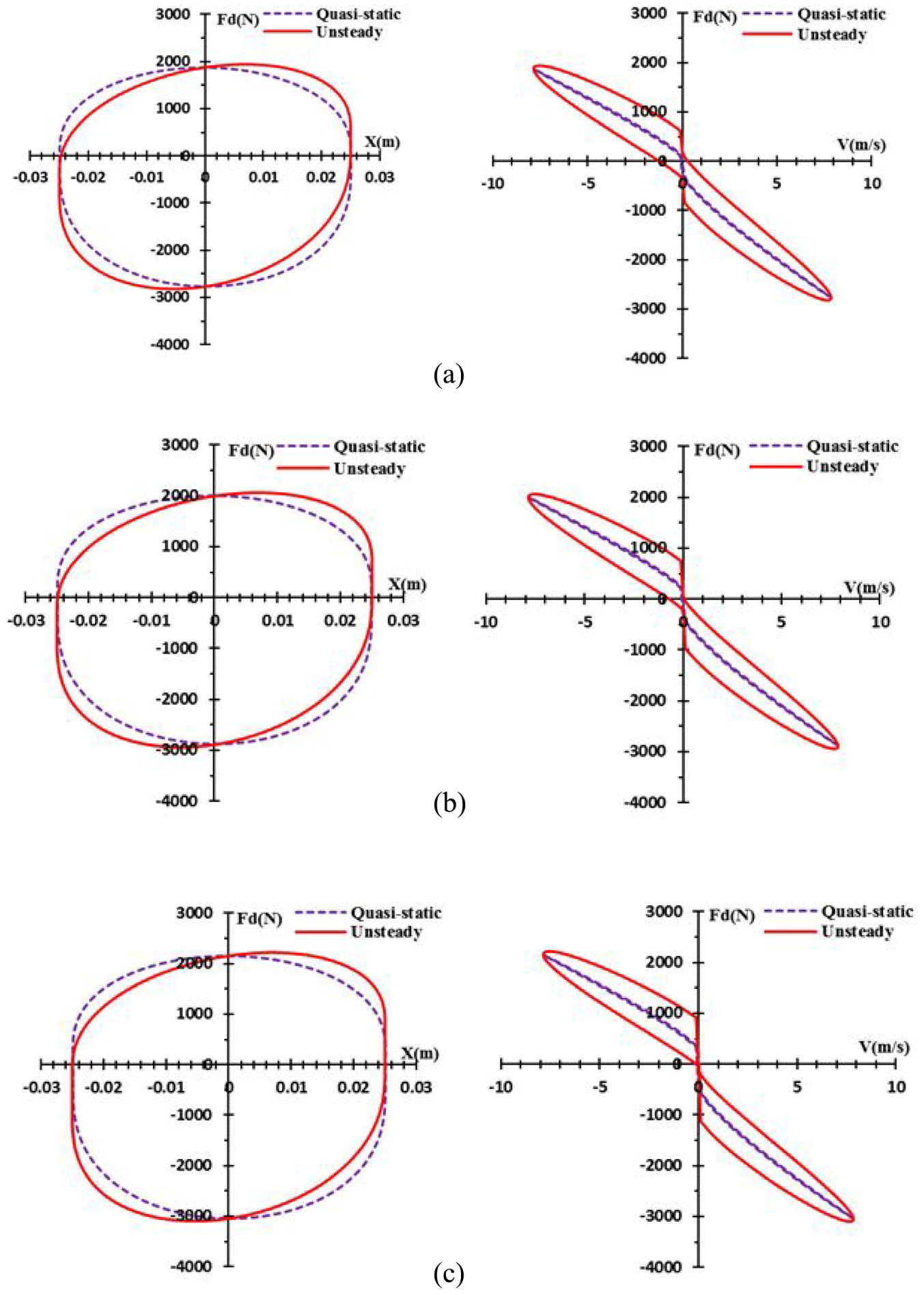
6.1.1. Force–displacement and force–velocity diagrams

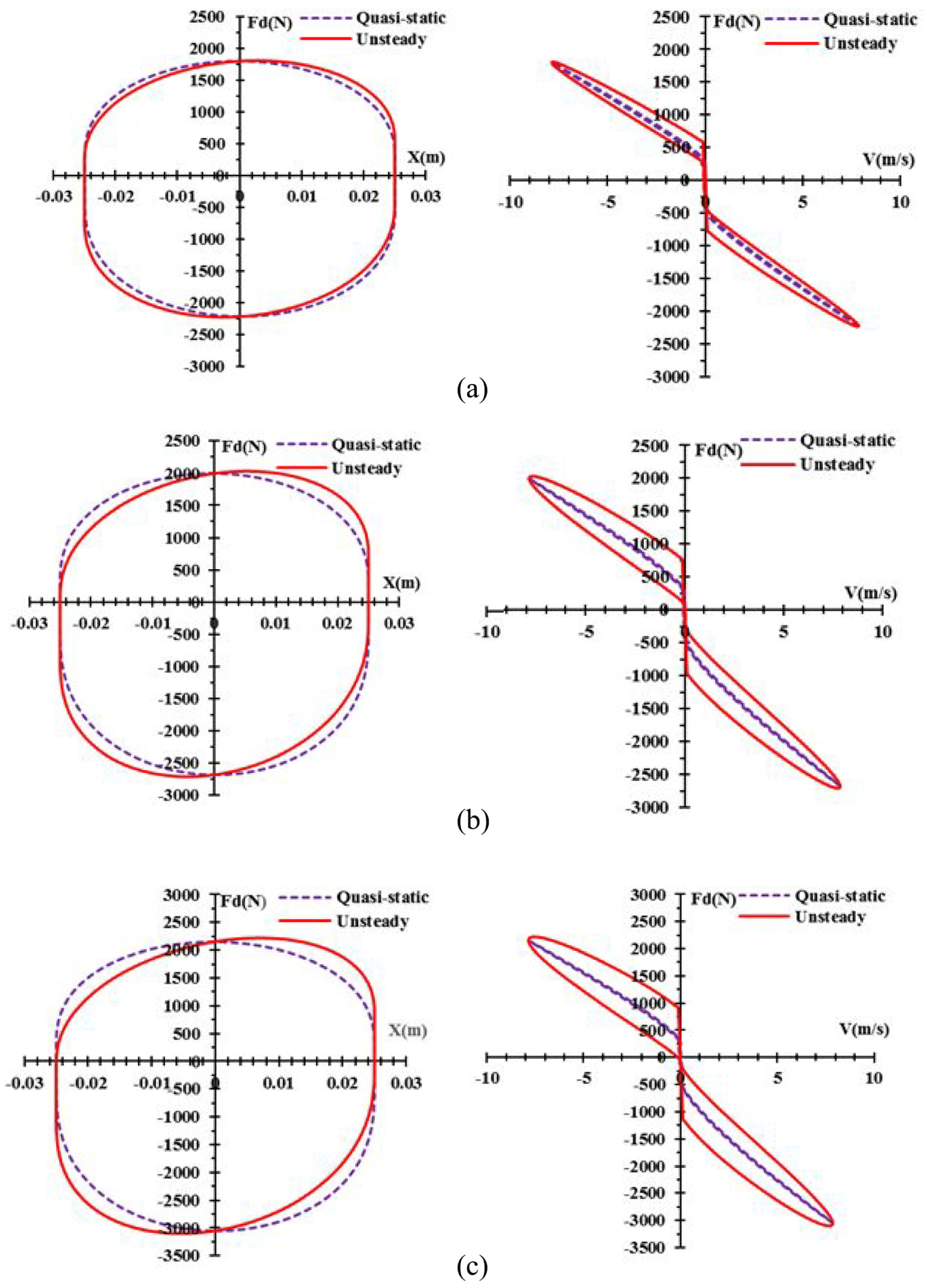
Force–displacement hysteresis loops of MR damper and also its damping force as a function of piston velocity are shown in Figures 7 and 8, respectively, for the frequency range of 0.636–50 Hz. It is clearly observable that the damping force is enhanced as the excitation frequency is increased. Also, one can infer from these figures that at low frequencies, the quasi-static analysis results and the new unsteady analysis results are in good agreement. But, by increasing the excitation frequency, the new unsteady analysis loops are deviated from the quasi-static analysis one. This deviation can be especially observed near the end of the storks where the fluid inertia is increased. For example, for f = 50 Hz, almost 180% error is included in quasi-static analysis results with respect to unsteady analysis results. It is due to the unsteady behavior of fluid flow via fluid inertia term influence on the momentum equation.

Figure 7.

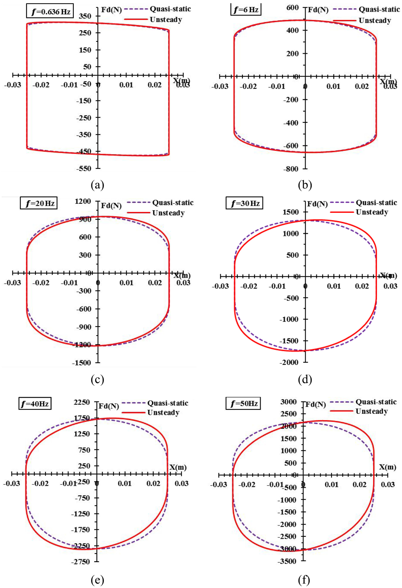
Force–displacement loops at (a) f = 0.636 Hz, (b) f = 6 Hz, (c) f = 20 Hz, (d) f = 30 Hz, (e) f = 40 Hz, and (f) f = 50 Hz (τ_y = 50 kPa; h_g = 0.0015 m; ρ = 3500 kg/m³; A = 0.025 m).

Figure 8.

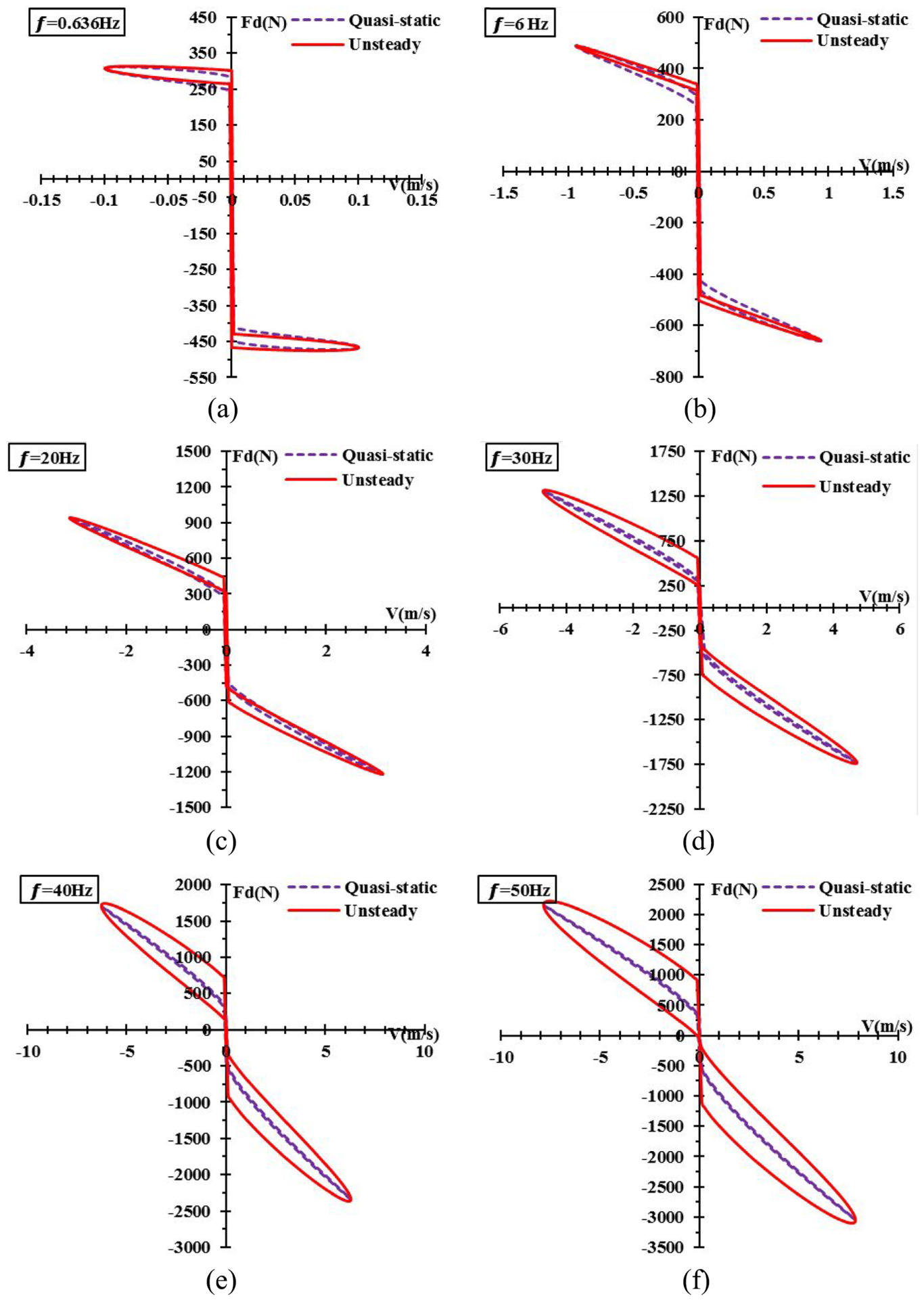
Force–velocity at (a) f = 0.636 Hz, (b) f = 6 Hz, (c) f = 20 Hz, (d) f = 30 Hz, (e) f = 40 Hz, and (f) f = 50 Hz (τ_y = 50 kPa; h_g = 0.0015 m; ρ = 3500 kg/m³; A = 0.025 m).

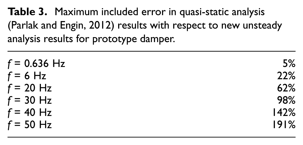
Also, maximum included error in quasi-static analysis results (Parlak and Engin, 2012) with respect to new unsteady analysis results for prototype damper at studied frequency range is given in Table 3. By increasing the excitation frequency, f, the inertia term increases significantly so error between quasi-static results and the present unsteady analysis is enhanced considerably. The errors between quasi-static results and the present unsteady analysis are due to neglecting the inertia term in quasi-static analysis.

Table 3.

Maximum included error in quasi-static analysis (Parlak and Engin, 2012) results with respect to new unsteady analysis results for prototype damper.

f = 0.636 Hz	5%
f = 6 Hz	22%
f = 20 Hz	62%
f = 30 Hz	98%
f = 40 Hz	142%
f = 50 Hz	191%

6.1.2. Phase difference between pressure drop and flow rate in gap

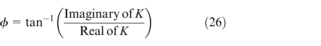
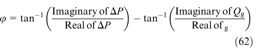
The variation of the phase difference between the total pressure drop and the flow rate can be predicted precisely, using the new unsteady analysis. It is a significant advantage of the new unsteady analysis rather than other unsteady (Chen et al., 2004; Nguyen and Choi, 2009; Yu et al., 2013) and quasi-static analyses (Ai et al., 2006; Brigley et al., 2007; Dimock et al., 2002; Ghaffari et al., 2014; Grunwald and Olabi, 2008; Hong et al., 2005, 2008; Kamath et al., 1996; Khan et al., 2014; Parlak and Engin, 2012; Phillips, 1969; Wang et al., 2009; Yang et al., 2002; Yoo and Wereley, 2005a, 2005b). This can be done by assuming velocity field, pressure gradient piston velocity and acceleration to be complex variables in the first step of the analysis. Therefore, as a result, the resultant pressure drop and flow rate should be complex values. Furthermore, the phase difference between the pressure drop and flow rate in all regions can be calculated using equation (62)

φ = \tan^{- 1} (\frac{Imaginary of Δ P}{Real of Δ P}) - \tan^{- 1} (\frac{Imaginary of Q_{g}}{{Real of}_{g}})

(62)

Based on this equation, time variation of the phase difference between pressure drop and flow rate for different values of the excitation frequency is shown in Figure 9. As shown in this figure, the phase difference between the Newtonian or viscous pressures drop and the flow rate, $φ_{N}$ , is time independent. It is obvious that at the lower frequencies, total phase difference, $φ_{t}$ , is more similar to the $φ_{MR}$ , and as the frequency is increased, the variation of total phase difference, $φ_{t}$ with time, is decreased and tends to $φ_{N}$ . Consequently, at the lower frequencies, the total pressure drop is more affected by MR effects (yield stress). Figure 10 shows the quasi-static and unsteady total pressure drop versus time for two frequencies, f = 0.636 and 50. It is clearly illustrated in this figure that the new unsteady analysis predicts precisely the variation of the phase difference between the total pressure drop and the flow rate. Furthermore, it is shown that by increasing the frequency, the quasi-static analysis fails to predict this phenomenon. It is due to incorporating fluid inertia term into the governing equations in new unsteady analysis. Also, it is obvious that the difference between quasi-static force–displacement and force–velocity diagrams and the unsteady one is due to phase difference that is caused by inertia term. This phenomenon can be explained as follows. Momentum equation for quasi-static and unsteady analysis is rewritten as equations (63) and (64):

Quasi-static condition

\frac{d P}{d x} = μ \frac{\partial^{2}}{\partial y^{2}} (U)

(63)

Unsteady condition

\frac{d P}{d x} = + μ \frac{\partial^{2}}{\partial y^{2}} (U) - ρ (\frac{\partial U}{\partial t})

(64)

Figure 9.

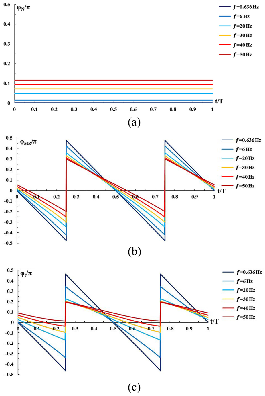
Phase difference between flow rate and pressure in (a) Newtonian regions of (b) non-Newtonian (MR) regions of gap, and (c) all regions of gap at different frequencies (τ_y = 50 kPa; h = 0.0015 m; ρ = 3500 kg/m³; A = 0.025 m).

Figure 10.

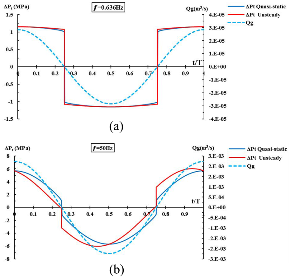
Time variation of flow rate and total pressure drop of gap (τ_y = 50 kPa; h = 0.0015 m; ρ = 3500 kg/m³; A = 0.025 m).

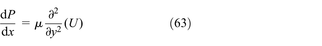
It can be inferred from these equations that in unsteady analysis, pressure gradient (pressure drop) is caused by shear stress and inertia term of fluid flow. Where, shear stress term is due to the viscosity and yield stress effects on the flow field. To investigate the effect of the inertia term on the phase difference between the pressure drop and the flow rate, first, quasi-static analysis of Newtonian fluid flow is considered. Equations (47) and (48) can be rewritten as follows

Q_{p} = A ω (A_{p} - A_{r}) \cos (ω t)

(65)

Δ P_{N} = \frac{12 μ L_{c}}{b h^{3}} A ω (A_{P} - A_{r} + bh) \cos (ω t)

(66)

According to equations (65) and (66), both the flow rate and the pressure drop are proportional to the cos(ωt) so there are in phase. According to equation (63), pressure drop caused by inertia term is neglected in quasi-static analysis. In the other word, in quasi-static analysis of Newtonian fluid flow, the total pressure drop just consists of the viscous pressure drop that is proportional to the flow rate.

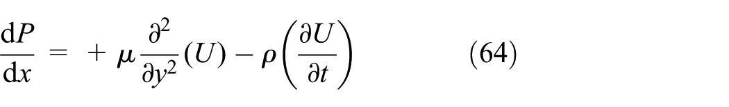
In the unsteady analysis of Newtonian fluid flow, according to equation (64), in addition to viscous shear stress, inertia term is incorporated into the governing equation too. Hence, pressure drop consists of acceleration pressure drop in addition to viscous pressure drop that is proportional to flow rate. It causes phase difference between the total pressure drop and the flow rate, as it can be inferred from Figure 9(a). According to this figure, as the frequency increases, the phase difference due to the acceleration pressure drop is increased. Also, equations (23) to (27) and (32) can be rewritten as equations (67) to (69)

Q_{g} = A ω (A_{P} - A_{r}) \exp (i ω t)

(67)

Δ P {(t)}_{N} = ρ L_{c} | K_{N} | \exp (i (ω t + ϕ_{N}))

(68)

Δ P {(t)}_{MR} = ρ L_{f} | K_{MR} | \exp (i (ω t + ϕ_{MR}))

(69)

According to these equations, in unsteady analysis, phase difference between the pressure drop and the flow rate, $φ$ (equation (62)), is related to the phase of K and $ϕ$ . It can be seen in Figure 9(a) that at low frequencies that velocity is nearly a quasi-static flow, phase difference between the total pressure drop and the flow rate is approximately equal to 0. However, at high frequencies (unsteady flow), phase of K and phase difference between the pressure drop and the flow rate, $φ$ , are affected by inertia term and increased. The magnitude and phase of K in unsteady analysis of Newtonian fluid flow are obtained directly from equation (24). In unsteady analysis of non-Newtonian (MRF) flow, three coupled nonlinear equations should be solved numerically to determine three unknown of K, y_pi, and y_po. Hence, magnitude and phase of K and so phase difference between the total pressure drop and the flow rate are dependent on boundaries of plug region and yield stress, in addition to inertia term and viscous shear stress. As shown in Figure 10, at high frequencies, quasi-static analysis fails to predict the effect of the inertia term on the phase of the K and so phase difference between the pressure drop and the flow rate, $φ$ . Which is mainly due neglecting inertia term in equation (63). Yield stress effects on velocity profile of equation (64), via boundary conditions of plug region that caused by yield stress.

6.1.3. Velocity profile of MRF flow

The velocity profile of the MRF flow inactive regions at t = T/8 is depicted in Figure 11(a). As shown in this figure, the higher the frequency, the larger the velocity magnitude. Also, the difference between the quasi-static and unsteady velocity profiles is clearly observed especially at higher frequencies. As the frequency increases, the post-yield regions are more developed in which the shear stress exceeds the yield stress. Also, by increasing the excitation frequency, the thickness of the plug flow region, where the shear stress is less than the yield stress, is decreased as it is illustrated in Figure 11(a). Consequently, as the frequency is increased, the MR damper working domain is more developed into the post-yield regions. The maximum deviation between the quasi-static and unsteady velocity profile is obtained in core region, where the inertia term is higher rather than near the walls, as it is observed in Figure 11(b).

Figure 11.

(a) Velocity profiles and (b) inertia term in MR regions for t = T/8 (τ_y = 50 kPa; h = 0.0015 m; ρ = 3500 kg/m³; A = 0.025 m).

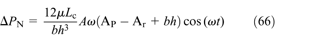
6.1.4. Variation of plug thickness with time

Plug thickness can be obtained from unsteady and quasi-static analysis using equations (34) and (53). As it is shown in Figures 11 and 12, for both unsteady and quasi-static analysis, plug thickness and non-dimensional plug thickness are decreased as the frequency is increased. Also, one can infer from these figures that unsteady plug thickness is smaller than quasi-static one, especially at higher frequencies. It is caused by the effect of inertia term in equation (34), which is neglected in quasi-static analysis (equation (55)). On the other hand, as it is observed in Figure 12(a), this deference is increased near the end of storks, where the inertia increases. The variation of inertia term of the plug region, with position of the piston, X(m) and frequency is shown in Figure 12(b). As it can be inferred from this figure, maximum inertia term magnitudes are near the end of the strokes, where the maximum error between the quasi-static and unsteady method results is obtained.

Figure 12.

Variation of (a) non-dimensional plug thickness with time at different frequencies, (b) inertia term of the plug region, with position of the piston, X(m) and frequency (τ_y = 50 kPa; h = 0.0015 m; ρ = 3500 kg/m³; A = 0.025 m).

6.2. Effect of yield stress

Damping force of the twin tube MR damper as a function of piston displacement and piston velocity is shown in Figure 13 for different yield stresses (15, 30, and 50 kPa). It is inferred from this figure that in larger yield stresses, the damping force is enhanced. It is also observed that the effect of fluid inertia and unsteady behavior of MRF flow are increased as the yield stress is decreased.

Figure 13.

Force–displacement and force–velocity loops at (a) τ_y = 15 kPa, (b) τ_y = 30 kPa, and (c) τ_y = 50 kPa (h = 0.0015 m; ρ = 3500 kg/m³; A = 0.025 m).

6.3. Effect of density

Figure 14 illustrates the effects of density of MRF on damping force, hysteresis dissipation, and characteristic loops of twin tube MR dampers. It can be seen that higher density results in higher dampening. On the other hand, as the density is increased, the effect of the unsteady behavior due to the MRF inertia on hysteresis dissipation and characteristic loops is increased and the deviation of unsteady behavior with respect to quasi-static one is also increased so unsteady behavior of dense MRFs is more significant.

Figure 14.

Force–displacement and force–velocity loops at (a) ρ = 1250 kg/m³, (b) ρ = 2500 kg/m³, and (c) ρ = 3500 kg/m³ (f = 50 Hz; h = 0.0015 m; τ_y = 50 kPa; A = 0.025 m).

6.4. Effect of gap height

The effects of gap height on damping force and unsteady behavior of the twin tube MR damper are shown in Figure 15. It is shown that as the gap height is decreased, the damping force is significantly increased and as a result, the difference between the quasi-static and unsteady analysis is increased.

Figure 15.

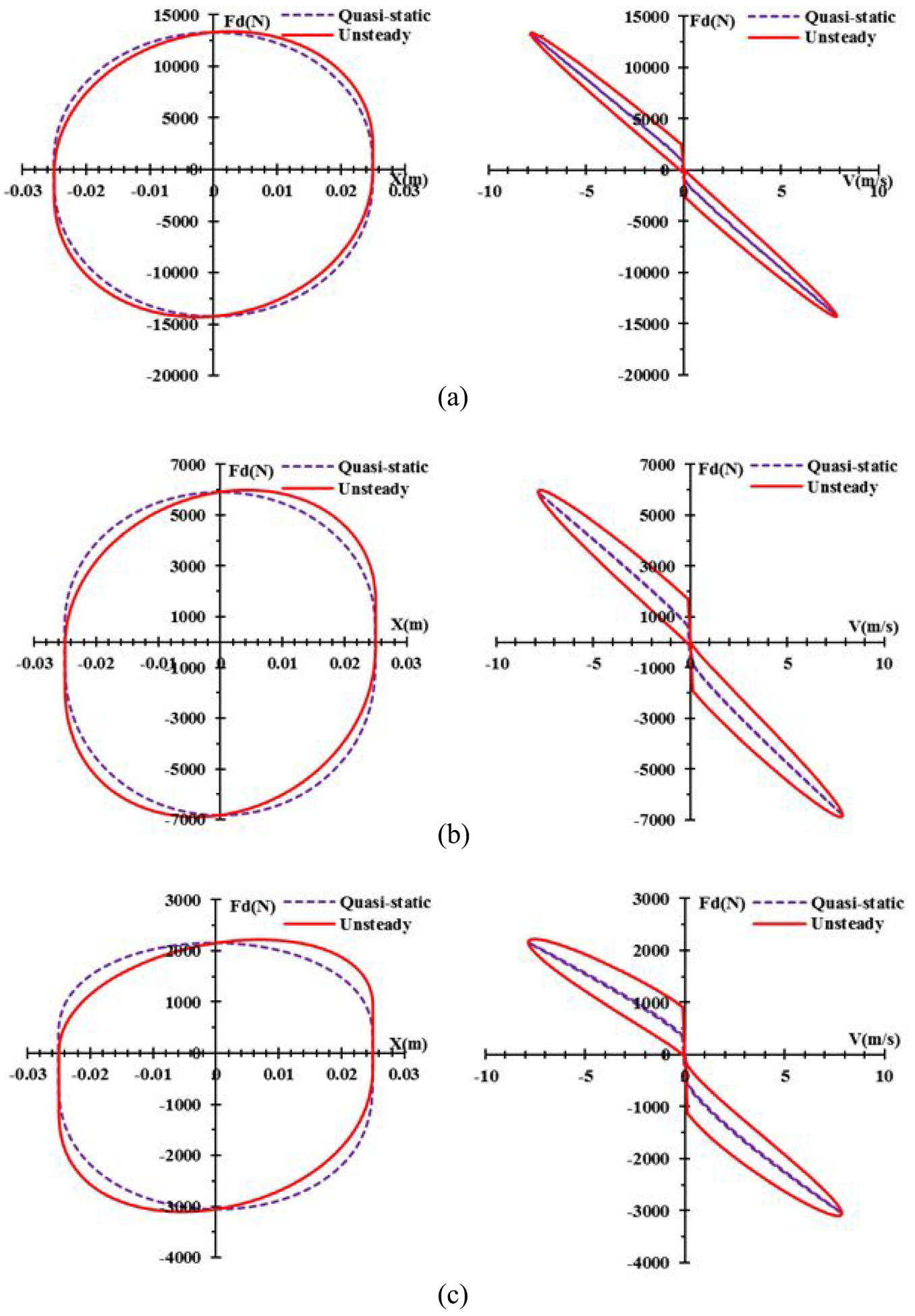
Force–displacement and force–velocity loops for (a) h = 0.0075 m, (b) h = 0.001 m, and (c) h = 0.0015 m (f = 50 Hz; ρ = 3500 kg/m³; τ_y = 50 kPa; A = 0.025 m).

6.5. Effect of oscillation amplitude

Damping force of the twin tube damper is affected by oscillation amplitude. The effect of oscillation amplitude on damping force, hysteresis dissipation, and unsteady behavior of the twin tube MR damper due to MRF inertia are depicted in Figure 16. It is obviously shown that the damping force and unsteady behavior of MRF are enhanced by increasing the oscillation amplitude. Furthermore, as the amplitude is increased, the maximum error of quasi-static behavior with respect to unsteady behavior is increased from 80% to 180%. As a result, one can deduce that as the amplitude increases, the effect of fluid inertia is increased.

Figure 16.

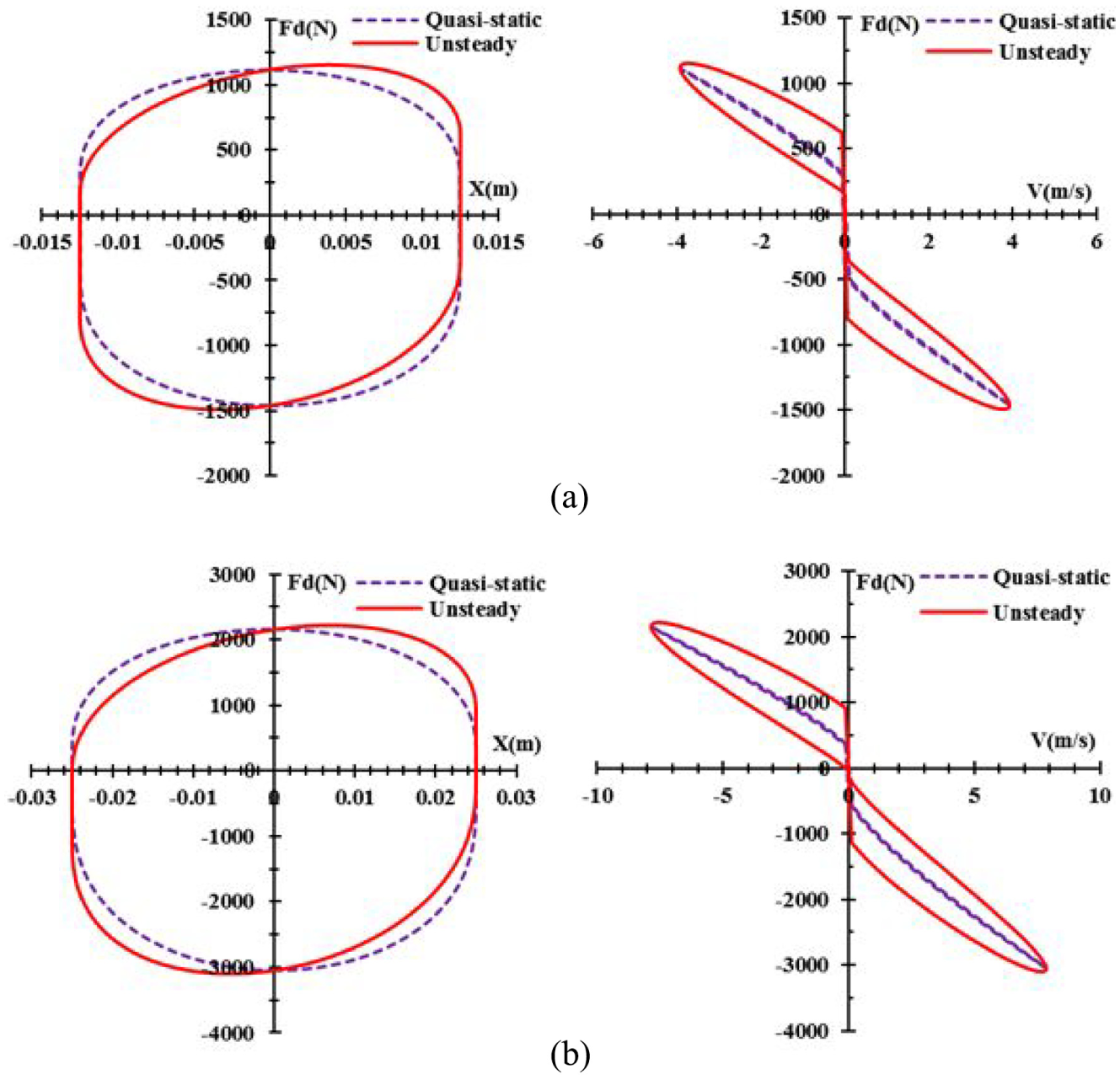
Force–displacement and force–velocity loops for (a) A = 0.0125 m and (b) A = 0.025 m (f = 50 Hz; ρ = 3500 kg/m³; τ_y = 50 kPa; h = 0.0015 m).

7. Conclusion

In this study, a new unsteady analysis based on Stokes’ second problem (Stokes, 1851) is developed for Bingham MRF flow through the annular gap which is opened on the piston head of twin tube MR damper. A quasi-static analysis is also developed for Bingham MRF flow through the annular gap inside the moving piston head.

According to the obtained results, as the excitation frequency, displacement amplitude, MRF density, and gap height are increased, the effects of MRF inertia on force–displacement and force–velocity loops are also increased and so, the deviation between the quasi-static analysis and the new unsteady analysis is increased. Furthermore, as the yield stress decreases, the effect of MRF inertia is increased. It can be inferred that at high frequencies, displacement amplitude and gap height have more effect on maximum damping force than the yield stress and density of MRF. A significant advantage of the new unsteady analysis with respect to other unsteady and quasi-static analyses is that the phase difference between pressure drop and flow rate along the gap can be easily calculated. In contrast with the quasi-static analysis which neglects the inertia term and so fails to predict the phase difference between the total pressure drop and the flow rate, the new unsteady analysis precisely predicts this phenomenon for higher frequencies.

Obtained results show that at lower frequencies, total phase difference value $φ_{t}$ is more close to the MR phase difference $φ_{MR}$ . Consequently, the total pressure drop is more affected by the MR effect (yield stress) at lower frequencies. In the non-Newtonian regions, it can be concluded from the obtained velocity profiles that for higher frequencies, the velocity profile is affected by the MRF inertia.

Furthermore, the results show that due to the effect of inertia term which is neglected in quasi-static analysis, the unsteady plug thickness is smaller than quasi-static one especially at higher frequencies and near the end of the strokes. Finally, the new unsteady analysis precisely predicts unsteady behavior of MRF flow and damper operation under unsteady state. Therefore, the authors believe that the new unsteady analysis can be used for design of MR devices instead of treating the more complex and expensive CFD simulations and experimental observations.

Footnotes

Declaration of conflicting interests

The author(s) declared no potential conflicts of interest with respect to the research, authorship, and/or publication of this article.

Funding

The author(s) received no financial support for the research, authorship, and/or publication of this article.

ORCID iD

M Norouzi

References

Wang

Liao

(2006) Design and modeling of a magnetorheological valve with both annular and radial flow paths. Journal of Intelligent Material Systems and Structures 17(4): 327–334.

Bird

Stewart

Lightfoot

(1960) Transport Phenomena. 2nd ed. New York: John Wiley & Sons.

Brigley

Choi

Y-T

Wereley

et al . (2007) Magnetorheological isolators using multiple fluid modes. Journal of Intelligent Material Systems and Structures 18(12): 1143–1148.

Burton

Makris

Konstantopoulos

et al . (1996) Modeling the response of ER damper: phenomenology and emulation. Journal of Engineering Mechanics 122(9): 897–906.

Chen

C-I

Chen

C-K

Yang

Y-T

(2004) Unsteady unidirectional flow of Bingham fluid between parallel plates with different given volume flow rate conditions. Applied Mathematical Modelling 28(8): 697–709.

Dimock

Yoo

J-H

Wereley

(2002) Quasi-steady Bingham biplastic analysis of electrorheological and magnetorheological dampers. Journal of Intelligent Material Systems and Structures 13(9): 549–559.

Dixon

(2007) The Shock Absorber Handbook. Chichester: John Wiley & Sons.

Ferdek

Luczko

(2012) Modeling and analysis of a twin-tube hydraulic shock absorber. Journal of Theoretical and Applied Mechanics 50(2): 627–638.

Gavin

(1998) Design method for high-force electrorheological dampers. Smart Materials and Structures 7(5): 664–673.

10.

Gavin

(2001) Annular Poiseuille flow of electrorheological and magnetorheological materials. Journal of Rheology 45(4): 983–994.

11.

Ghaffari

Hashemabadi

Ashtiani

(2014) A review on the simulation and modeling of magnetorheological fluids. Journal of Intelligent Material Systems and Structures 26(8): 881–904.

12.

Grunwald

Olabi

(2008) Design of magneto-rheological (MR) valve. Sensors and Actuators A: Physical 148(1): 211–223.

13.

Hong

Choi

et al . (2005) Non-dimensional analysis and design of a magnetorheological damper. Journal of Sound and Vibration 288(4–5): 847–863.

14.

Hong

Wereley

Choi

et al . (2008) Analytical and experimental validation of a nondimensional Bingham model for mixed-mode magnetorheological dampers. Journal of Sound and Vibration 312(3): 399–417.

15.

Jolly

Bender

Carlson

(1999) Properties and applications of commercial magnetorheological fluids. Journal of Intelligent Material Systems and Structures 10(1): 5–13.

16.

Kamath

Hurt

Wereley

(1996) Analysis and testing of Bingham plastic behavior in semi-active electrorheological fluid dampers. Smart Materials and Structures 5(5): 576–590.

17.

Khan

Suresh

Seetharamaiah

(2014) Principles, characteristics and applications of magneto rheological fluid damper in flow and shear mode. Procedia Materials Science 6: 1547–1556.

18.

Kreyszig

(1983) Advanced Engineering Mathematics. New York: John Wiley & Sons.

19.

Nguyen

Q-H

Choi

S-B

(2009) Dynamic modeling of an electrorheological damper considering the unsteady behavior of electrorheological fluid flow. Smart Materials and Structures 18(5): 055016.

20.

Parlak

Engin

(2012) Time-dependent CFD and quasi-static analysis of magnetorheological fluid dampers with experimental validation. International Journal of Mechanical Sciences 64(1): 22–31.

21.

Phillips

(1969) Engineering applications of fluids with a variable yield stress. PhD Thesis, University of California, Berkeley, CA.

22.

Soda

Iwata

Sunakoda

et al . (2001) Experimental and analytical methods for predicting mechanical properties of MRF damper. In: Proceeding of the Smart structures and materials 2001: smart systems for bridges, structures, and highways, Newport Beach, CA, 5–7 March, pp. 201–212. International Society for Optics and Photonics.

23.

Sternberg

Zemp

Llera

JCDL

(2014) Multiphysics behavior of a magneto-rheological damper and experimental validation. Engineering Structures 69: 194–205.

24.

Stokes

(1851) On the Effect of the Internal Friction of Fluids on the Motion of Pendulums. Cambridge: Pitt Press.

25.

Wang

Liao

(2009) A magnetorheological valve with both annular and radial fluid flow resistance gaps. Smart Materials and Structures 18(11): 115001.

26.

Wereley

Pang

(1998) Nondimensional analysis of semi-active electrorheological and magnetorheological dampers using approximate parallel plate models. Smart Materials and Structures 7(5): 732–743.

27.

White

(2006) Viscous Fluid Flow. New York: McGraw-Hill.

28.

Yang

Spencer

Carlson

et al . (2002) Large-scale MR fluid dampers: modeling and dynamic performance considerations. Engineering Structures 24(3): 309–323.

29.

Yoo

J-H

Wereley

(2005a) Nondimensional analysis of annular duct flow in magnetorheological/electrorheological dampers. In: Proceeding of the electrorheological fluids and magnetorheological suspensions (ERMR 2004), Beijing, China, 29 August–3 September, pp. 1577–1583. Hackensack, NJ: World Scientific.

30.

Yoo

J-H

Wereley

(2005b) Quasi-steady axisymmetric Bingham-plastic model of magnetorheological flow damper behavior. In: ASME 2005 International mechanical engineering congress and exposition, Orlando, FL, 5–11 November, pp. 375–380. New York: American Society of Mechanical Engineers.

31.

Wang

et al . (2013) Unsteady analysis for oscillatory flow of magnetorheological fluid dampers based on Bingham plastic and Herschel–Bulkley models. Journal of Intelligent Material Systems and Structures 24(9): 1067–1078.

Parametric investigation of twin tube magnetorheological dampers using a new unsteady theoretical analysis

Abstract

Keywords

1. Introduction

2. Problem statement

3. Governing equations and constitutive equation

4. Unsteady analysis

4.1. Determining the velocity field

4.1.1. Newtonian regions

4.1.2. Non-Newtonian (MR) regions

4.2. Obtaining pressure drop in Newtonian regions

4.3. Obtaining pressure drop, ypi and ypo, in non-Newtonian (MR) regions

4.3.1. Continuity equation

4.3.2. Continuity of velocity profile at boundaries of plug region

4.3.3. Force equilibrium for plug region

4.4. Damping force

5. Quasi-static analysis

5.1. Velocity in Newtonian regions

5.2. Pressure drop in Newtonian regions

5.3. Velocity in non-Newtonian (MR) region

5.4. Pressure drop in non-Newtonian regions

6. Results and discussion

6.1. Effect of frequency

6.1.1. Force–displacement and force–velocity diagrams

6.1.2. Phase difference between pressure drop and flow rate in gap

6.1.3. Velocity profile of MRF flow

6.1.4. Variation of plug thickness with time

6.2. Effect of yield stress

6.3. Effect of density

6.4. Effect of gap height

6.5. Effect of oscillation amplitude

7. Conclusion

Footnotes

Declaration of conflicting interests

Funding

ORCID iD

References

4.3. Obtaining pressure drop, y_pi and y_po, in non-Newtonian (MR) regions