Thermomechanical description of shape memory alloys using constitutive models with assumed polynomial phase transformation kinetics

Abstract

Shape memory alloys present remarkable thermomechanical behaviors due to solid phase transformations. The complexity of the involved phenomena makes the constitutive modeling of this class of smart material a challenging subject. Considering the different approaches presented in the literature, the constitutive models with assumed phase transformation kinetics are popular, achieving reasonable results. This paper deals with one-dimensional constitutive models that employs a novel strategy to describe phase transformation kinetics using polynomial functions. Three different polynomial functions are treated: linear, quadratic, and cubic. Besides, the novel approach defines the phase transformation surfaces in such a way that allows the description of new phenomena including tension-compression behaviors and two-way shape memory effect. Experimental data compiled from the literature guides the investigation treating temperature-induced phase transformation; pseudoelasticity; one-way and two-way shape memory effects; internal subloops due to incomplete phase transformations. Numerical simulations are carried out comparing the novel functions with the classical cosine function. Results indicate that the model with polynomial phase transformation kinetics is able to capture the main features of SMA thermomechanical behavior. The investigation shows that the cubic polynomial is equivalent to the cosine function and the linear polynomial presents good estimations, being related to low computational cost since it avoids iterative approaches for strain-driven cases.

Keywords

shape memory alloys pseudoelasticity shape memory effect constitutive models phase transformation kinetics

Introduction

Shape memory alloys (SMAs) are active, functional, smart materials with unique capabilities related to the thermomechanical couplings of solid-solid martensitic phase transformations (Lagoudas, 2008). SMAs have been employed in several applications exploiting two main characteristics associated with hysteretic behavior: shape memory effect, related to large recoverable strains induced by thermomechanical loadings; and pseudoelasticity or superelasticity, associated with large strains and high dissipation capacity (Savi et al., 2016; Thomas et al., 2025).

Aerospace industry is one of the most important fields of SMA applications (Hartl and Lagoudas, 2007; Leal and Savi, 2018; Silva et al., 2022). Nevertheless, the literature presents many other areas including oil and gas industry (Liu et al., 2024b; Silva et al., 2021), robotics (Kim et al., 2023; Pan et al., 2025; Ruth et al., 2022), and biomedical applications (Chaudhary et al., 2024; Machado and Savi, 2003; Sima et al., 2024). Recently, SMA morphing structures have evolved to employ origami-inspired structures (Fonseca et al., 2022; Peraza-Hernandez et al., 2014), being related to different kinds of innovations. Additional discussions of SMA applications in different areas are presented in Jani et al. (2014), Gantz et al. (2022), Dalave et al. (2024), and Kumar et al. (2024).

Temperature-dependent behavior of SMA can be employed to provide adaptiveness to mechanical systems (Nozaki et al., 2021). Since the SMA properties vary with phase and therefore with temperature, stiffness change is exploited in distinct situations including dynamical applications (Savi, 2015; Sohn et al., 2023). Rotordynamics is an example where temperature changes promote the adaptive behavior of rotor systems, allowing the control of critical speeds (Jin et al., 2024; Preto et al., 2023). The synergistic use of smart materials is another application with a growing interest. In this regard, the combination of SMAs with piezoelectric materials allows the development of adaptive energy harvesters with enhanced capabilities (Adeodato et al., 2021; Liu et al., 2021).

Hysteretic dissipation is also employed in dynamical applications (Savi, 2015; Tabrizikahou et al., 2022). This dissipation is useful in civil structures, especially the ones subjected to severe loads as earthquakes (Fang, 2022; Liu et al., 2024a; Vignoli et al., 2020). Stroud and Hartl (2023) proposed an innovative application of SMA wires to construct a 2D knitted structure to be subjected to high loads. Del Core et al. (2025) investigated the use of SMAs to preserve historical structures.

The effectiveness of SMA to mitigate crack growth propagation in steel structures was demonstrated by Wang et al. (2024) and Li et al. (2025). Debossan and Vignoli (2022) presented finite element simulations indicating that the inclusion of SMA layers can avoid impact damage in composite plates. Wang et al. (2025) proposed an analytical model for the impact behavior in SMAs based on the wave propagation theory. The benefits of including SMA reinforcement in composite plates subjected to impact loads was also demonstrated by Brack and Ghasemnejad (2025).

The SMA modeling is associated with distinct approaches focused on different scales and due to several phenomena involved (Lagoudas, 2008; Shaw and Kyriades, 1995; Wang et al., 2021), is a complex task. An overview of the most relevant constitutive models to describe the macroscopic behavior of SMAs is presented by Paiva and Savi (2006), Lagoudas (2008), Khandelwal and Buravalla (2009), Cisse et al. (2016a, 2016b), and Chowdhury (2018). Multiscale perspective is discussed by Liu and Dong (2024) that employed a three-phase micromechanical model while Zhu et al. (2025) discussed a molecular dynamics simulation to evaluate the influence of porosity.

Data-driven multidisciplinar models were also proposed as an interesting alternative to describe SMA thermomechanical behavior, presenting simplicity as the main characteristics (Honrao et al., 2023; Trehern et al., 2022). The Preisach model should be highlighted to describe generalized hysteresis (Alvares et al., 2024; Mayergoyz, 2003), being also employed for different smart materials. Recently, Dornelas et al. (2025, 2026) proposed a novel prismatic approach that generalizes the Preisach model to incorporate distinct phenomena. This new approach allows the description of temperature-dependent behavior and more complex phenomena as transformation induced plasticity. Artificial neural networks are also a possibility to for data-driven models (Wang and Wang, 2021).

Regarding the SMA constitutive models, the models with internal constraints present a solid mechanical foundation based on continuum mechanics and thermodynamics. In this regard, several approaches can be identified based on plasticity theoretical framework (Auricchio and Sacco, 1997; Souza et al., 1998; Yang et al., 2023), phase transformation forces (Boyd and Lagoudas, 1996), and Fremond’s theory (Dornelas et al., 2021; Fremond, 1987; Oliveira et al., 2016; Paiva et al., 2005). It should be pointed out the challenges related to the description of complex phenomena that includes transformation induced plasticity, classical plasticity, rate-dependent behavior, functional and structural fatigue, among others, which are even more complex considering three-dimensional media.

There is a class of constitutive models with assumed phase transformation kinetics that are attractive due to their simplicity and good match with experimental data. The pioneer work of Tanaka and Nagaki (1982), Tanaka (1985), Tanaka et al. (1986), and Tanaka et al. (1994) assumed an exponential function to describe the phase transformation kinetics, allowing a proper constitutive description of SMAs. Afterward, other alternative functions were proposed by Liang and Rogers (1990), Boyd and Lagoudas (1994) and Ivshin and Pence (1994), typically considering cosine functions. Brinson (1993) improved this class of model by considering different perspectives. Although the model is still using the cosine function, two variants of martensite were introduced: twinned and detwinned. Besides, different properties for each phase were adopted, enhancing the SMA description.

He et al. (2023) proposed a modification of the Brinson’s model using different cosine functions for a better description of the experimental behavior. Ren et al. (2007) used the error function, Wang et al. (2019) proposed hyperbolic functions, and Zhang et al. (2024) considered logistic functions. Adeodato et al. (2022) considered quadratic polynomial function split into two phase transformation regions. Despite the undeniable advances related to SMA modeling, the simplification for engineering applications is still desirable, as claimed by Medina et al. (2023).

This paper deals with a novel one-dimensional classified in the group of assumed phase transformation kinetics model. Polynomial functions are employed to describe the phase transformation kinetics, evaluating linear, quadratic, and cubic polynomials. Besides, novel phase transformation surfaces are defined in such a way that allows the description of new phenomena including tension-compression behaviors and two-way shape memory effect. Numerical simulations are carried out to describe the main thermomechanical behaviors of SMAs: pseudoelasticity, shape memory effect – one- and two-way, temperature-induced phase transformation and internal subloops. A comprehensive analysis of polynomial phase transformations is developed using experimental data compiled from the literature, attesting the model capabilities. Results are compared with the classical cosine function, showing that the polynomial function is an interesting alternative to describe SMA phase transformation kinetics.

After this introduction, the mathematical formulation of the constitutive models is presented in Section 2. The details related to the numerical implementations are presented in Section 3. The models are compared with four sets of experimental data compiled from the literature in Section 4. Finally, the main conclusions are summarized in Section 5.

SMA constitutive models with assumed kinetics

SMA remarkable characteristics are related to thermomechanical couplings represented by different phenomena. Phase transformation is the main phenomenon behind the macroscopic behavior of SMAs and two distinct phases should be identified: austenite, stable at high temperatures in stress-free state; and martensite, stable at low temperatures in stress-free state. Austenite is related to only one variant while martensite can present several variants where preferential cases are defined from external stress field.

The macroscopic thermomechanical behavior of SMAs is described by constitutive models that needs to be thermodynamically consistent. On this basis, it needs to respect the second law of thermodynamics, represented by the Clausius-Duhen inequality (Lemaitre and Chaboche, 1990). State variables are needed to establish this description, and it is usual to consider the strain, ε, and the temperature, T, as the observable variables. Besides, internal variables should be defined to describe phase transformations and the martensitic volume fraction, β, is usually employed.

By considering that the martensitic volume fraction is split into two variants, $β = β_{σ} + β_{T}$ , where $β_{σ}$ is the stress-induced detwinned martensite and $β_{T}$ is the temperature-induced twinned martensite, the constitutive equation can be presented in rate form as follows (Brinson, 1993):

\overset{\cdot}{σ} = E \overset{\cdot}{ε} - Ω {\overset{\cdot}{β}}_{σ} - γ \overset{\cdot}{T}

(1)

where the dot indicates the time derivative; E is the elastic modulus; Ω is the phase transformation parameter; and γ is the coefficient related to thermal expansion. Note that the parameter Ω can be estimated from the maximum recoverable strain, $ε_{M}$ , in such a way that $Ω = E ε_{M}$ . The parameter γ is related to the thermal expansion coefficient, α, by the expression $γ = E α$ .

In general, properties are different for each phase and therefore, they need to be defined by a kind of rule of mixtures. On this basis, it is possible to write:

E = E_{A} + β (E_{M} - E_{A})

(2)

α = α_{A} + β (α_{M} - α_{A})

(3)

where M represents martensite and A represents austenite.

The phase transformation kinetics is represented by a function $β = β (σ, T)$ and the choice of this function defines the different models with assumed phase transformation kinetics. In essence, $β = 0$ represents a situation with the presence of 100% of austenitic phase (A) while $β = 1$ represents the presence of 100% of martensitic phase (M). Nevertheless, a broader perspective can be given for this variable in order to represent tensile and compressive martensitic variants. Therefore, it is possible to consider a domain $[- 1, + 1]$ instead of $[0, 1]$ , and on this basis, $β = + 1$ represents the tensile detwinned martesite (M+), while $β = - 1$ represents the compressive detwinned martesite (M−).

The critical stresses and temperatures that define phase transformations need to be identified by a critical phase transformation surface. By considering the stress-driven austenite-martensite (forward) transformation $A \to M$ , critical stress levels are defined from the start and finish values $σ_{M_{s}}$ and $σ_{M_{f}}$ , respectively, whereas temperature-induced transformation has critical start and finish temperatures defined by $M_{s}$ and $M_{f}$ , respectively. On the other hand, the stress-driven martensite-austenite (reverse) transformation $M \to A$ , the critical values are $σ_{A_{s}}$ and $σ_{A_{f}}$ ; and similarly, temperature-induced transformations are represented by the temperature values: $A_{s}$ and $A_{f}$ . The representation of these critical values can be experimentally determined, being expressed in a phase transformation critical surface illustrated in Figure 1. Further explanations of the experimental approach used to obtain these parameters are presented in Section 3. In general, the following expressions can be employed to characterize the phase transformation critical values:

σ_{A_{s}} = σ_{TW} + C_{A} (T - A_{s})

(4)

σ_{A_{f}} = σ_{TW} + C_{A} (T - A_{f})

(5)

σ_{M_{s}} = σ_{TW} + σ_{s} + C_{M} (T - M_{s})

(6)

σ_{M_{f}} = σ_{TW} + σ_{f} + C_{M} (T - M_{f})

(7)

where $C_{A}$ and $C_{M}$ are material parameters; $σ_{s}$ and $σ_{f}$ define the constant stress level for martensitic low temperature behavior; and $σ_{TW}$ is a residual stress field. For the sake of simplicity, $σ_{TW} = 0$ is adopted in Figure 1.

Figure 1.

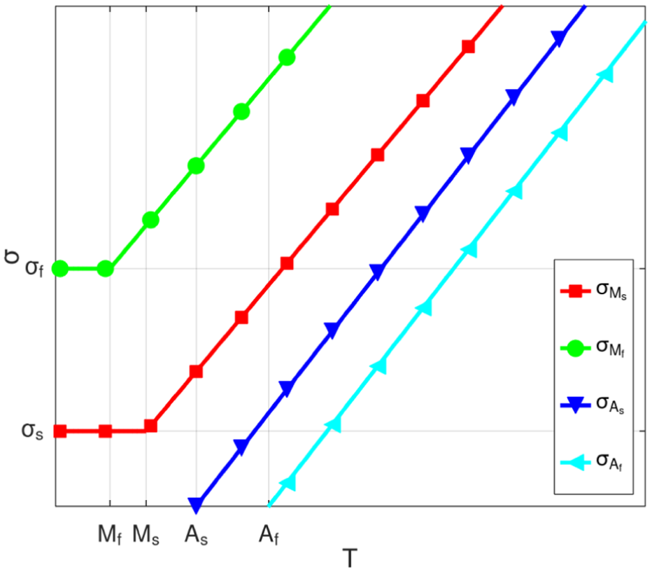
Phase transformation critical surfaces based on Brinson (1993).

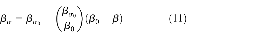
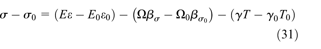
The inclusion of the residual stress field $σ_{TW}$ is a novel strategy to describe the two-way shape memory effect. This field is induced by a training thermomechanical process necessary to make an SMA sample to present this phenomenon. Typically, this process is modeled by considering permanent plastic strain induced during the two-way shape memory effect training process (Hakimi and Ashrafi, 2023; Scalet et al., 2019). The alternative here proposed is simpler assuming the residual stress field induced by the training process.

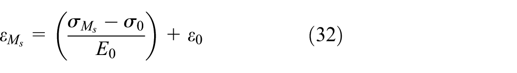
It can be established that the stress-induced austenite-martensite transformation occurs when the condition $σ_{Ms} < σ < σ_{M_{f}}$ is satisfied. Additionally, the following functions are defined to represent the transformation kinetics:

β_{σ} = (\frac{1 - β_{σ_{0}}}{2}) f_{M} (σ, T) + (\frac{1 + β_{σ_{0}}}{2})

(8)

β_{T} = β_{T_{0}} - (\frac{β_{T_{0}}}{1 - β_{σ_{0}}}) (β_{σ} - β_{σ_{0}}) + (\frac{1 - β_{T_{0}}}{2}) g_{M} (T)

(9)

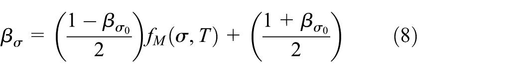
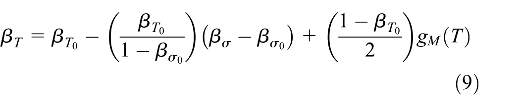
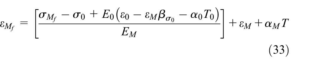
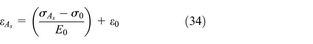
where the subscript “0” denotes the quantities in the initial state; $f_{M} (σ, T)$ is a function that satisfies $f_{M} (σ_{M_{s}}, T) = - 1$ and $f_{M} (σ_{M_{f}}, T) = 1$ . Note that $β_{σ} = β_{σ_{0}}$ if $f_{M} (σ_{M_{s}}, T) = - 1$ , and $β_{σ} = 1$ if $f_{M} (σ_{M_{f}}, T) = 1$ . Additionally, if $M_{f} < T < M_{s}$ and $\overset{\cdot}{T} < 0$ , the function $g_{M} (T)$ must satisfy the conditions $g_{M} (M_{f}) = 2$ and $g_{M} (M_{s}) = 0$ ; otherwise, $g_{M} (T) = 0$ .

For the stress-induced martensite-austenite transformation, it can be established that the condition $σ_{A_{f}} < σ < σ_{A_{s}}$ must be satisfied to occur phase transformation and the kinetics is represented by the following functions:

β = (\frac{β_{0}}{2}) h_{A} (σ, T)

(10)

β_{σ} = β_{σ_{0}} - (\frac{β_{σ_{0}}}{β_{0}}) (β_{0} - β)

(11)

β_{T} = β_{T_{0}} - (\frac{β_{T_{0}}}{β_{0}}) (β_{0} - β)

(12)

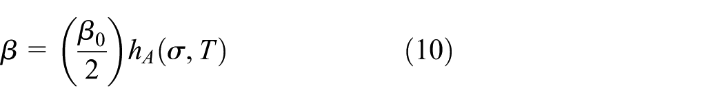
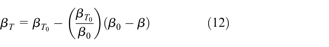
where $h_{A} (σ, T)$ is a function that satisfies $h_{A} (σ_{A_{s}}) = 2$ and $h_{A} (σ_{A_{f}}) = 0$ .

Therefore, the phase transformation kinetics is described by the functions $f_{M} (σ, T)$ , $g_{M} (T)$ , and $h_{A} (σ, T)$ , which characterizes the different models in the literature. In the sequel, the classical Brinson’s model functions are presented followed by the novel polynomials model functions that are proposed in this work.

Brinson’s model

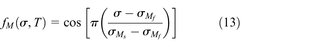
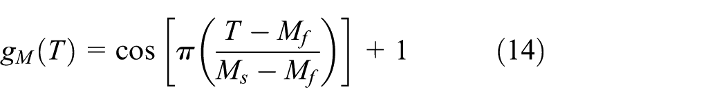
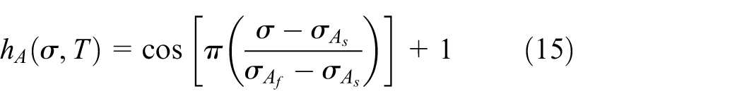
The assumed function for the phase transformation kinetics is the key for the SMA constitutive description. The pioneer work of Tanaka and Nagaki (1982) employed an exponential function, but the cosine alternatives were employed in several references with a good performance (Boyd and Lagoudas, 1994; Ivshin and Pence, 1994; Liang and Rogers, 1990). Brinson (1993) proposed the following cosine functions to represent phase transformation kinetics:

f_{M} (σ, T) = \cos [π (\frac{σ - σ_{M_{f}}}{σ_{M_{s}} - σ_{M_{f}}})]

(13)

g_{M} (T) = \cos [π (\frac{T - M_{f}}{M_{s} - M_{f}})] + 1

(14)

h_{A} (σ, T) = \cos [π (\frac{σ - σ_{A_{s}}}{σ_{A_{f}} - σ_{A_{s}}})] + 1

(15)

Polynomial models

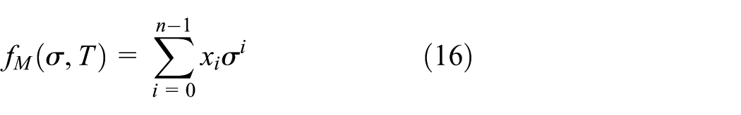
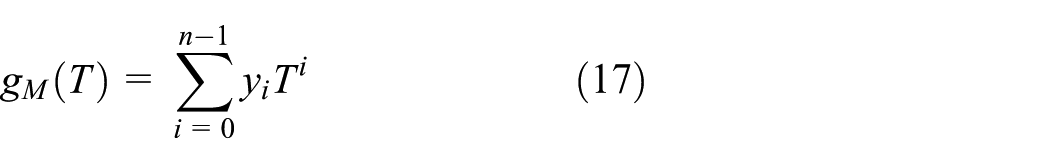
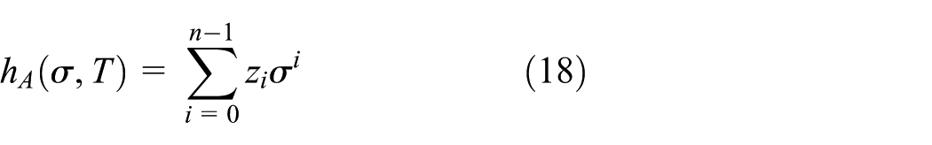
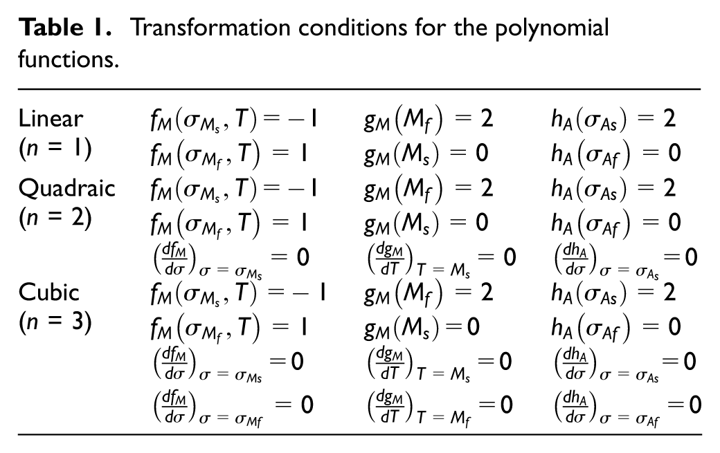
This work proposes the use of polynomial functions for the SMA phase transformation kinetics. In a general way, different polynomial order functions are employed, using transformation conditions to define the coefficients. In this regard, the following equations are adopted:

f_{M} (σ, T) = \sum_{i = 0}^{n - 1} x_{i} σ^{i}

(16)

g_{M} (T) = \sum_{i = 0}^{n - 1} y_{i} T^{i}

(17)

h_{A} (σ, T) = \sum_{i = 0}^{n - 1} z_{i} σ^{i}

(18)

where $x_{i}$ , $y_{i}$ , and $z_{i}$ are unknown to be evaluated according to phase transformation conditions, and n is the order of the polynomial function. A summary of the phase transformation conditions is presented in Table 1 for linear, quadratic and cubic polynomials. Once the transformation conditions are imposed, it is necessary to solve a linear system according to the degree of the polynomial.

Table 1.

Transformation conditions for the polynomial functions.

Linear (n = 1)	$f_{M} (σ_{M_{s}}, T) = - 1$	$g_{M} (M_{f}) = 2$	$h_{A} (σ_{As}) = 2$
Linear (n = 1)	$f_{M} (σ_{M_{f}}, T) = 1$	$g_{M} (M_{s}) = 0$	$h_{A} (σ_{Af}) = 0$
Quadraic (n = 2)	$f_{M} (σ_{M_{s}}, T) = - 1$	$g_{M} (M_{f}) = 2$	$h_{A} (σ_{As}) = 2$
	$f_{M} (σ_{M_{f}}, T) = 1$	$g_{M} (M_{s}) = 0$	$h_{A} (σ_{Af}) = 0$
	${(\frac{{df}_{M}}{d σ})}_{σ = σ_{M_{s}}} = 0$	${(\frac{{dg}_{M}}{dT})}_{T = M_{s}} = 0$	${(\frac{{dh}_{A}}{d σ})}_{σ = σ_{A_{s}}} = 0$
Cubic (n = 3)	$f_{M} (σ_{M_{s}}, T) = - 1$	$g_{M} (M_{f}) = 2$	$h_{A} (σ_{As}) = 2$
	$f_{M} (σ_{M_{f}}, T) = 1$	$g_{M} (M_{s}) = 0$	$h_{A} (σ_{Af}) = 0$
	${(\frac{{df}_{M}}{d σ})}_{σ = σ_{Ms}} = 0$	${(\frac{{dg}_{M}}{dT})}_{T = M_{s}} = 0$	${(\frac{{dh}_{A}}{d σ})}_{σ = σ_{As}} = 0$
	${(\frac{{df}_{M}}{d σ})}_{σ = σ_{Mf}} = 0$	${(\frac{{dg}_{M}}{dT})}_{T = M_{f}} = 0$	${(\frac{{dh}_{A}}{d σ})}_{σ = σ_{Af}} = 0$

On this basis, each polynomial kinetics is discussed in the sequel.

Linear polynomial

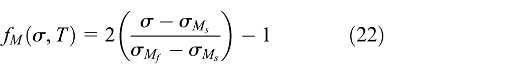
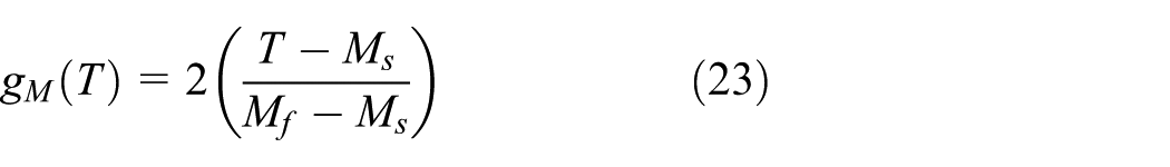
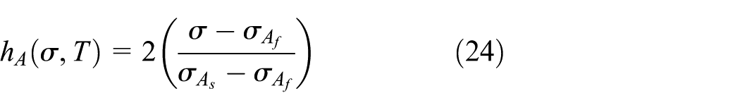
The linear polynomial phase transformation kinetics considers a function of the form,

f_{M} (σ, T) = x_{1} σ + x_{0}

(19)

g_{M} (T) = y_{1} T + y_{0}

(20)

h_{A} (σ, T) = z_{1} σ + z_{0}

(21)

By applying the transformation conditions, it is reached the following functions:

f_{M} (σ, T) = 2 (\frac{σ - σ_{M_{s}}}{σ_{M_{f}} - σ_{M_{s}}}) - 1

(22)

g_{M} (T) = 2 (\frac{T - M_{s}}{M_{f} - M_{s}})

(23)

h_{A} (σ, T) = 2 (\frac{σ - σ_{A_{f}}}{σ_{A_{s}} - σ_{A_{f}}})

(24)

Quadratic polynomial

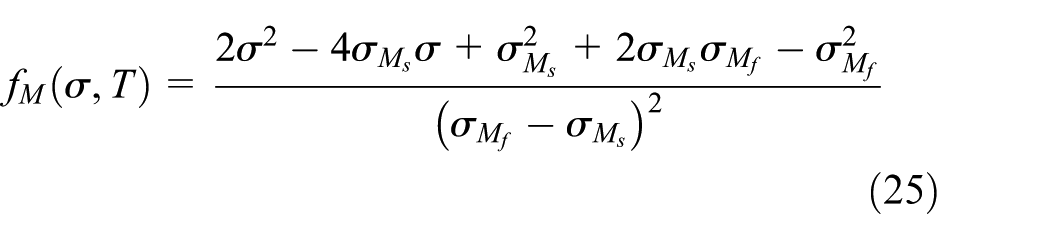
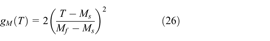
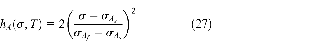
The quadratic polynomial phase transformation kinetics considers a quadratic function and, by applying the phase transformation conditions, the following equations are obtained considering analogous procedure of the linear polynomial,

f_{M} (σ, T) = \frac{2 σ^{2} - 4 σ_{M_{s}} σ + σ_{M_{s}}^{2} + 2 σ_{M_{s}} σ_{M_{f}} - σ_{M_{f}}^{2}}{{(σ_{M_{f}} - σ_{M_{s}})}^{2}}

(25)

g_{M} (T) = 2 {(\frac{T - M_{s}}{M_{f} - M_{s}})}^{2}

(26)

h_{A} (σ, T) = 2 {(\frac{σ - σ_{A_{s}}}{σ_{A_{f}} - σ_{A_{s}}})}^{2}

(27)

Cubic polynomial

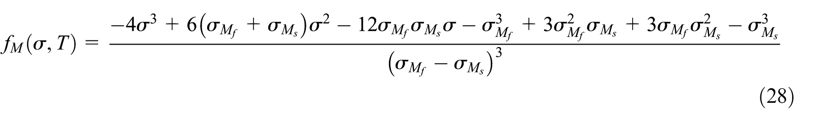
The cubic polynomial phase transformation kinetics considers a third order function and, by applying the phase transformation conditions, the following equations are obtained,

f_{M} (σ, T) = \frac{- 4 σ^{3} + 6 (σ_{M_{f}} + σ_{M_{s}}) σ^{2} - 12 σ_{M_{f}} σ_{M_{s}} σ - σ_{M_{f}}^{3} + 3 σ_{M_{f}}^{2} σ_{M_{s}} + 3 σ_{M_{f}} σ_{M_{s}}^{2} - σ_{M_{s}}^{3}}{{(σ_{M_{f}} - σ_{M_{s}})}^{3}}

(28)

g_{M} (T) = \frac{- 4 T^{3} + 6 (M_{f} + M_{s}) T^{2} - 12 M_{f} M_{s} T + 2 M_{s} (3 M_{f} - M_{s})}{{(M_{f} - M_{s})}^{3}}

(29)

h_{A} (T) = \frac{4 σ^{3} - 6 (σ_{A_{f}} + σ_{A_{s}}) σ^{2} + 12 σ_{A_{f}} σ_{A_{s}} σ + 2 σ_{A_{s}} (σ_{A_{f}} - 3 σ_{A_{s}})}{{(σ_{A_{f}} - σ_{A_{s}})}^{3}}

(30)

Parameter characterization

This section presents details about the SMA characterization, showing the experimental tests developed to define the constitutive parameters. Essentially, material characterization is performed by considering thermomechanical tests. The evaluation of phase transformation temperatures employs differential scanning calorimeter (DSC) while mechanical properties are defined from quasi-static tensile tests performed in a testing machine.

In order to present the material characterization, experimental tests are carried out on a pseudoelastic Ni56Ti44 (wt.%) wire in its as-received condition, manufactured by Sandinox Biomaterials. The wire has a circular cross-section with a diameter of 1.3 mm. A DSC NETZSCH Maia 200 F3 is employed together with quasi-static tensile tests using an Instron 5882 electromechanical testing machine equipped with a 30 kN static load cell and displacement-based strain measurement employing a gage length of 100 mm. A thermal chamber is also employed to conduct tests at various temperatures.

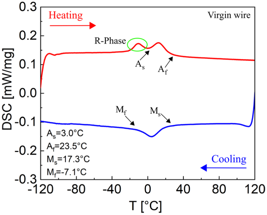
The analysis of the phase transformation temperatures is conducted through DSC tests using a virgin wire sample. The sample is heated from room temperature to 120°C and subsequently cooled to −120°C, repeating this thermal cycle. Figure 2 presents results of the test, highlighting the transformation temperatures of the start and finish of austenitic formation ( $A_{s}$ , $A_{f}$ ) and the start and finish of martensitic formation ( $M_{s}$ , $M_{f}$ ). During the heating process, two distinct phase transformation regions are observed: the transition from martensite to R-phase, followed by the conversion of R-phase to austenite. During cooling, a pronounced transformation peak marks the reverse transition from austenite to martensite. For temperatures above $A_{f}$ (23.5°C), the austenitic phase is stable, and the sample presents a pseudoelastic behavior when subjected to mechanical loading. On the other hand, for temperatures below $M_{f}$ (−7.1°C), the martensite phase is stable, and the SMA presents the shape memory effect.

Figure 2.

Phase transformation temperatures through DSC thermal analysis of the virgin NiTi wire.

After the thermal analysis, mechanical characterization is of concern. Initially, the cyclic response of the SMA sample is assessed by subjecting a specimen to a training process using a quasi-static cyclic tensile test, conducted at a peak stress of 900 MPa with a stress rate of 150 MPa/min. The training involves repeated cyclic mechanical loading until a stabilized response is achieved. This stabilization process is related to the transformation induced plasticity (TRIP) strain stabilization that ensures the repeatability of the material behavior throughout the cycles (Oliveira et al., 2018). Figure 3(a) illustrates the stress-strain curves obtained over 29 cycles, highlighting the comparison between the first and last cycles showing the TRIP strain stabilization, the progressive reduction of hysteresis loop size, and the decrease of critical stresses associated with phase transformations. In addition, Figure 3(b) presents the strain evolution of the specimen throughout the cycles, revealing that stabilization occurs after approximately 20 cycles.

Figure 3.

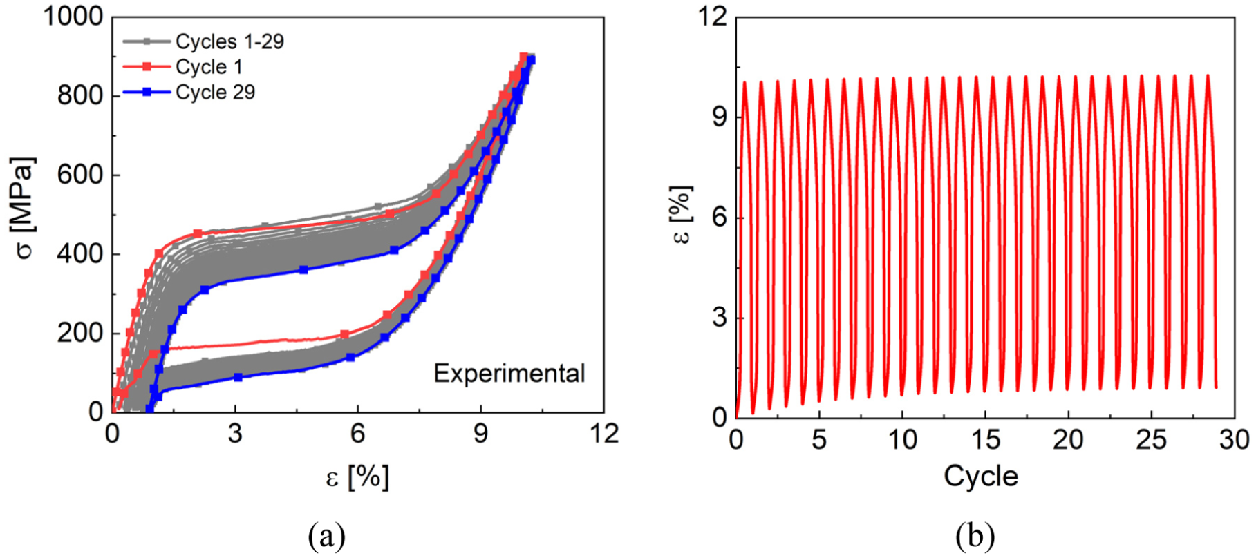
Training procedure of a pseudoelastic NiTi wire at a temperature of 30°C, at a maximum stress of 900 MPa, and a loading rate of 150 MPa/min: (a) cyclic stress-strain response and (b) TRIP strain stabilization throughout the cycles.

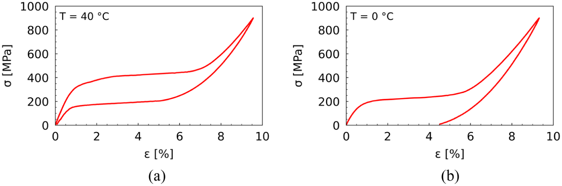
After the training procedure, a macroscopic evaluation of the SMA mechanical behavior is conducted based on the stress-strain curves at different temperatures. Figure 4 presents stress-strain curve at 40°C (above $A_{f}$ ) and 0°C (between $M_{s}$ and $M_{f}$ ). Results highlight the distinct thermomechanical responses of the sample under these conditions, showing a pseudoelastic behavior at 40°C. On the other hand, at 0°C, the shape memory effect is observed, presenting an incomplete phase transformation during unloading.

Figure 4.

Stress-strain curves considering different temperatures conducted from a sample initially trained at 30°C, considering a maximum stress of 900 MPa, and a loading rate of 150 MPa/min: (a) 40°C and (b) 0°C.

The SMA characterization needs to define all the constitutive parameters including phase transformation critical stress for direct ( $σ_{M_{s}}$ and $σ_{M_{f}}$ ) and reverse ( $σ_{A_{s}}$ and $σ_{A_{f}}$ ) phase transformations by using the tangent method. This approach involves the identification of the intersection of tangent lines corresponding to the regions where phase transformations start and finish, as presented in Figure 5(a) for a pseudoelastic test at 40°C. The elastic modulus of the austenitic phase ( $E_{A}$ ) is determined by the angular coefficient of the elastic region of austenite, during the loading process. On the other hand, the elastic modulus of the martensitic phase ( $E_{M}$ ) is determined by the angular coefficient of elastic region of martensite, during unloading. The slope is calculated using selected data points in the elastic regions as illustrated in Figure 5(b). The maximum residual strain $ε_{M}$ is achieved when the austenite undergoes complete transformation into detwinned martensite for a shape memory effect test. Upon unloading, this strain remains unchanged until the temperature is increased above $A_{s}$ . The determination of $ε_{M}$ is performed by considering a tangent line in the region where the unloading occurs, and this tangent line is extended until it reaches the horizontal axis, as shown in Figure 5(c) for a test at 0°C.

Figure 5.

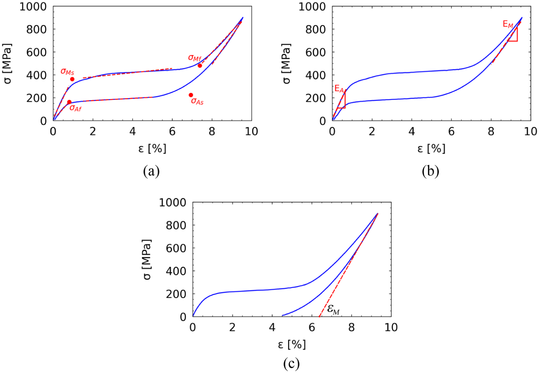
SMA constitutive parameters: (a) critical stresses, (b) elastic modulus for austenite and martensite, and (c) maximum recoverable strain $ε_{M}$ .

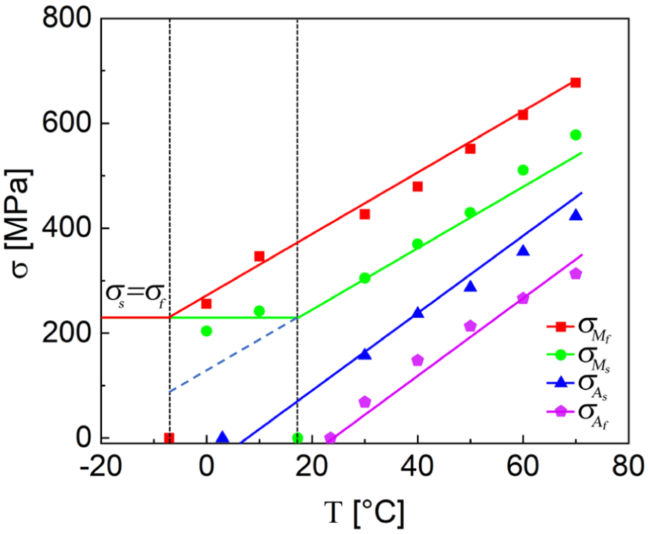
Phase transformations are defined from the critical transformation surfaces. The relationship among temperature and phase transformation critical stresses is defined by constants $C_{A}$ and $C_{M}$ . Their experimental determination involves the procedure illustrated in Figure 5(a) across various temperatures, combined with the experimental test shown in Figure 2, which identifies the phase transformation temperatures in the absence of mechanical loading. Figure 6 presents results measured by tensile tests at different temperatures: 0°C, 10°C, 30°C, 40°C, 50°C, 60°C, and 70°C. Besides, phase transformation temperatures obtained from DSC tests are employed to define the temperature values for stress-free states. Linear regression for each phase transformation critical stress is employed allowing the determination of parameters $C_{A}$ and $C_{M}$ .

Figure 6.

Phase transformation critical surfaces.

Considering temperatures below $M_{f}$ , in the absence of mechanical loading, only the twinned martensite variant is present. When a mechanical load is applied, a reorientation process occurs, transforming the twinned martensite into detwinned martensite, which starts at the stress $σ_{s}$ and finishes at $σ_{f}$ . The constants $σ_{s}$ and $σ_{f}$ represent material parameters that can be experimentally estimated by considering parallel lines derived from the intersections of the critical stresses $σ_{M_{s}}$ and $σ_{M_{f}}$ with the respective phase transformation temperatures $M_{s}$ and $M_{f}$ . The intersection of these lines with the vertical axis provides the value of $σ_{s}$ and $σ_{f}$ . This procedure is illustrated in Figure 6. The residual stress field $σ_{TW}$ is generated by a two-way shape memory alloy training process and can be macroscopically evaluated by adjusting the strain recovery induced by temperature changes (Hakimi and Ashrafi, 2023; Scalet et al., 2019).

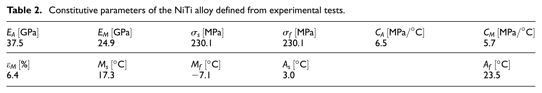
Based on these tests and related approaches, the SMA is characterized, and all constitutive parameters are defined. Table 2 summarizes all these parameters.

Table 2.

Constitutive parameters of the NiTi alloy defined from experimental tests.

$E_{A} [GPa]$	$E_{M} [GPa]$	$σ_{s} [MPa]$	$σ_{f} [MPa]$	$C_{A}$ [MPa/°C]	$C_{M}$ [MPa/°C]
37.5	24.9	230.1	230.1	6.5	5.7
$ε_{M} [%]$	M_s [°C]	M_f [°C]	A_s [°C]		A_f [°C]
6.4	17.3	−7.1	3.0		23.5

Numerical procedure

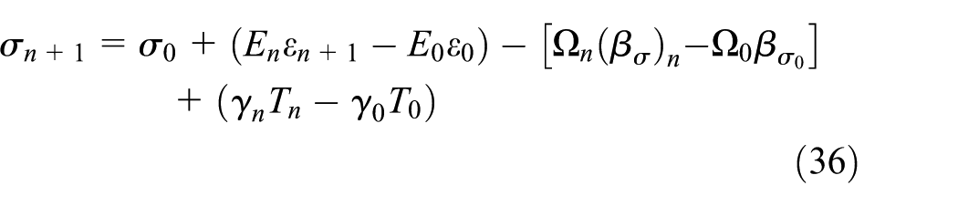
The numerical implementation of the constitutive equations considers a time integration that allows to write the following discrete version that should be evaluated together with the assumed function for transformation kinetics:

σ - σ_{0} = (E ε - E_{0} ε_{0}) - (Ω β_{σ} - Ω_{0} β_{σ_{0}}) - (γ T - γ_{0} T_{0})

(31)

Analysis can be performed by considering stress-driven, temperature-driven, and strain-driven cases and the essential point is the definition of phase transformation domains. On this basis, stress-driven and temperature-driven cases allow a direct determination of the phase transformation surfaces since they are defined by stress-temperature functions and both are known.

On the other hand, strain-driven cases need to use a predictor-corrector algorithm, estimating a trial stress that allows the evaluation of the transformation surfaces. From both information, the actual state is defined. This methodology is a typical predictor-corrector approach.

The classical return-mapping algorithm is an example of a predictor-corrector approach for plasticity (Simo and Hugles, 1998) while the projection algorithm is its counterpart for phase transformations (Oliveira et al., 2016). Essentially, a trial elastic state is defined followed by an evaluation of an inelastic evolution; if there is an inelastic evolution, a correction is needed, and the trial state is corrected by a projection that leads to the actual state. The classical plasticity promotes the projection to the yield surface and the inelastic evolution is related to plastic strains. On the other hand, the phase transformation problem needs to promote the projection to the phase transformation surfaces and the inelastic evolution is related to volume fraction evolution.

By considering the strain-driven phase transformation case, the inelastic evolution needs to define the phase transformation surfaces, characterized by unknown strain bounds since they are defined from stress values. Therefore, assuming an elastic step from a known previous state, a trial state is defined by considering that phase transformation does not occur. The trial stress allows the evaluation of phase transformation surface and, if the strain is inside the inelastic domain, the actual state should be recalculated estimating the martensitic volume fraction, which requires an iterative process to solve a nonlinear equation. A projection algorithm can be employed and alternatively, an optimization algorithm can be implemented to minimize the difference between the trial and actual states.

Golden section algorithm

Phase transformations are essentially characterized by the critical stress values for the start and finish of these transformations. Therefore, the martensitic transformations are defined by $σ_{M_{s}}$ and $σ_{M_{f}}$ , while austenite is defined by $σ_{A_{s}}$ and $σ_{A_{f}}$ . For strain-driven cases, it becomes useful to define the strain values associated with these stresses to evaluate if there is phase transformation or if the material has an elastic behavior. Thus, the strains for start and finish phase transformations are defined by the following expressions

ε_{M_{s}} = (\frac{σ_{M_{s}} - σ_{0}}{E_{0}}) + ε_{0}

(32)

ε_{M_{f}} = [\frac{σ_{M_{f}} - σ_{0} + E_{0} (ε_{0} - ε_{M} β_{σ_{0}} - α_{0} T_{0})}{E_{M}}] + ε_{M} + α_{M} T

(33)

ε_{A_{s}} = (\frac{σ_{A_{s}} - σ_{0}}{E_{0}}) + ε_{0}

(34)

ε_{A_{f}} = [\frac{σ_{A_{f}} - σ_{0} + E_{0} (ε_{0} - ε_{M} β_{σ_{0}} - α_{0} T_{0})}{E_{A}}] + α_{A} T

(35)

In order to introduce the algorithm, consider a known state ( $σ_{n}$ , $ε_{n}$ , $β_{n}$ ), and its evolution to an unknown state ( $σ_{n + 1}$ , $ε_{n + 1}$ , $β_{n + 1}$ ) considering $ε_{n + 1} = ε_{n} + Δ ε$ . If $ε_{n + 1}$ is outside inelastic domain (defined by the bonds of phase transformation), the actual state is defined by considering that $β_{n + 1} = β_{n}$ , which means that $E_{n + 1} = E_{n}$ , $Ω_{n + 1} = Ω_{n}$ , and $γ_{n + 1} = γ_{n}$ . Hence, the stress is computed by

\begin{matrix} σ_{n + 1} = σ_{0} + (E_{n} ε_{n + 1} - E_{0} ε_{0}) - [Ω_{n} {(β_{σ})}_{n} - Ω_{0} β_{σ_{0}}] \\ + (γ_{n} T_{n} - γ_{0} T_{0}) \end{matrix}

(36)

Otherwise, if $ε_{n + 1}$ is inside the inelastic domain, an iterative procedure is required. By assuming a trial stress state, $σ_{n + 1}^{trial}$ , the martensite volume fraction can be computed by defining $β_{n + 1}^{trial} = β (σ_{n + 1}^{trial})$ using the equations previously presented in Section 2 for each model. Consequently, the SMA elastic modulus and coefficient of thermal expansion are also obtained for the trial solution since they are functions of the martensite volume fraction. In other words, if $σ_{n + 1}^{trial}$ is estimated, $E_{n + 1}^{trial}$ , $Ω_{n + 1}^{trial}$ , and $γ_{n + 1}^{trial}$ can be calculated. This conclusion implies that the nonlinear problem can be rewritten as a problem of finding the roots of the following function:

\begin{matrix} F = (σ_{n + 1}^{trial} - σ_{0}) - (E_{n + 1}^{trial} ε_{n + 1} - E_{0} ε_{0}) \\ + [Ω_{n + 1}^{trial} {(β_{σ})}_{n + 1}^{trial} - Ω_{0} β_{σ_{0}}] + (γ_{n + 1}^{trial} T_{n + 1} - γ_{0} T_{0}) \end{matrix}

(37)

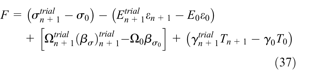
Note that $F = F (σ_{n + 1}^{trial})$ is a one-variable function. Additionally, the domain limits are $σ_{M_{s}} \leq σ_{n + 1}^{trial} \leq σ_{M_{f}}$ for the austenite-martensite transformation, and $σ_{A_{s}} \geq σ_{n + 1}^{trial} \geq σ_{A_{f}}$ for the martensite-austenite transformation.

To find the root of F that satisfies the limit conditions associated with the critical stresses, the golden section method is applied (Ji et al., 2022; Koupaei et al., 2016). First, the lower and upper limits of the trial stress solution are defined as $σ_{lower}$ and $σ_{upper}$ , respectively, where $σ_{lower} = σ_{M_{s}}$ and $σ_{upper} = σ_{M_{f}}$ for the transformation to detwinned martensite, and $σ_{lower} = σ_{A_{f}}$ and $σ_{upper} = σ_{A_{s}}$ for the transformation to austenite.

Four different points are evaluated within the domain $σ_{lower} \leq σ_{n + 1}^{trial} \leq σ_{upper}$ :

{σ_{n + 1}^{trial}}_{1} = σ_{lower}

(38)

{σ_{n + 1}^{trial}}_{2} = σ_{lower} + (1 - R_{A}) (σ_{upper} - σ_{lower})

(39)

{σ_{n + 1}^{trial}}_{3} = σ_{lower} + R_{A} (σ_{upper} - σ_{lower})

(40)

{σ_{n + 1}^{trial}}_{4} = σ_{upper}

(41)

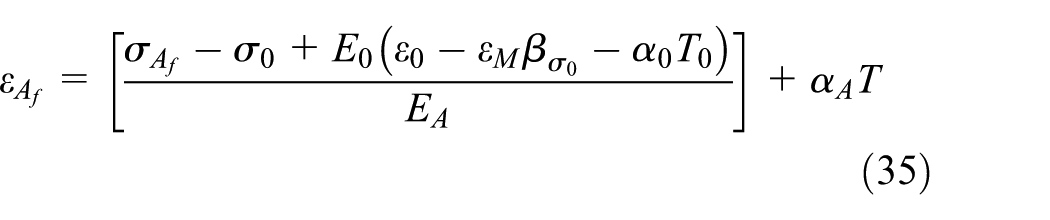
where $R_{A} = (\sqrt{5} - 1) / 2$ is the golden ratio.

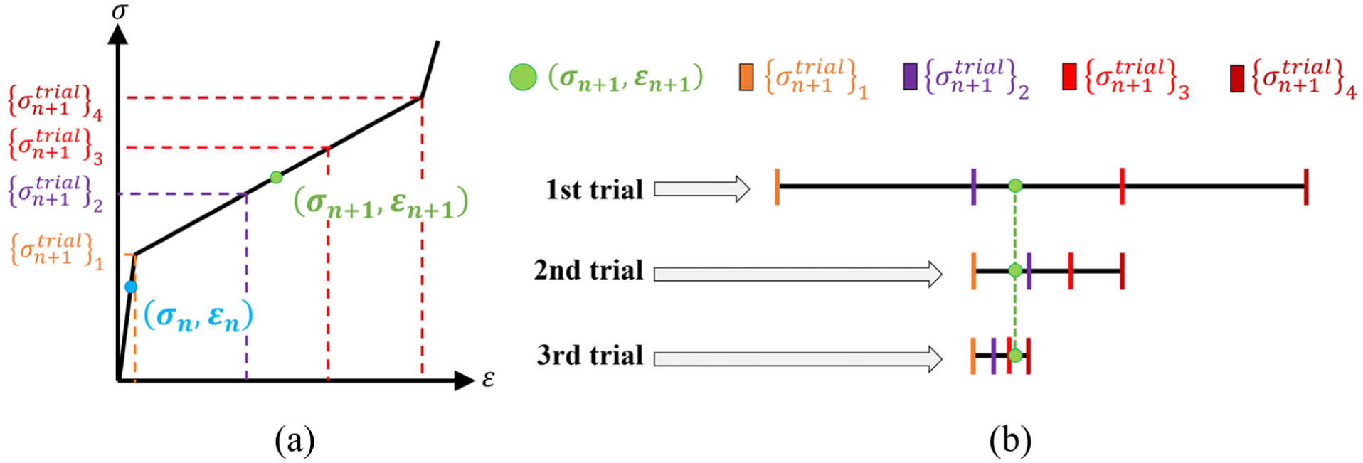
Once the trial stress solutions are defined using equations (38)–(41), these parameters are replaced into equation (37) to compute the values of $F ({σ_{n + 1}^{t r i a l}}_{i})$ . The method consists in recursively update the values of $σ_{lower}$ and $σ_{upper}$ according to signal of $F ({σ_{n + 1}^{t r i a l}}_{i})$ . For an illustrative example, Figure 7(a) shows the stress-strain curve considering that the previous state is in the elastic regime and the actual state is in the inelastic domain with phase transformation. The recursive procedure is illustrated in Figure 7(b), where the first three iterations updating the values of $σ_{lower}$ and $σ_{upper}$ are also represented. Computational iterations are performed until the convergence is reached, when the absolute value of $F ({σ_{n + 1}^{t r i a l}}_{i})$ becomes smaller than the tolerance.

Figure 7.

Schematic representation of the golden section algorithm: (a) stress-strain curve considering the previous state ( $σ_{n}, ε_{n})$ , and the actual state ( $σ_{n + 1}, ε_{n + 1}$ ) and (b) iterative approach to find roots of F updating the values of $σ_{lower}$ and $σ_{upper}$ .

Linear phase transformation kinetics

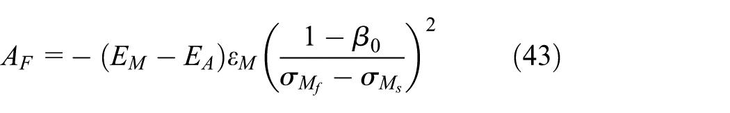
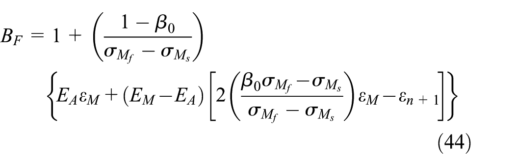
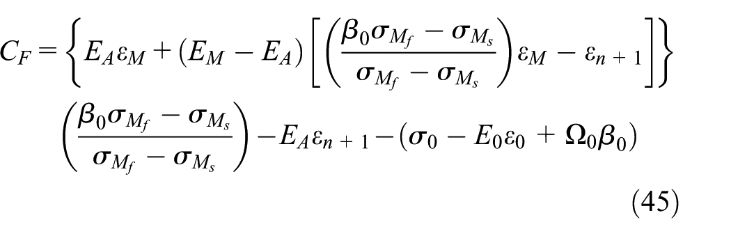
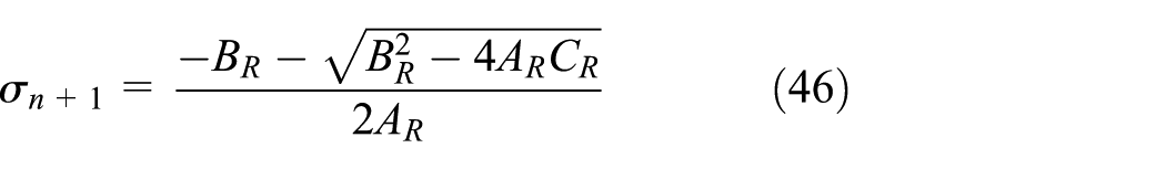
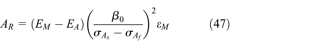
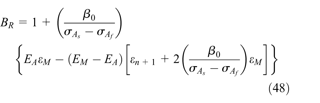
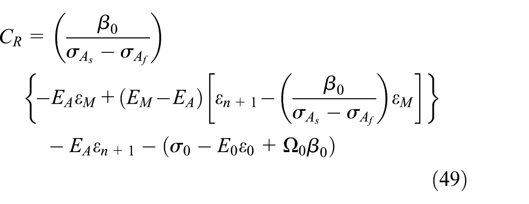
By considering the linear polynomial kinetics, an analytical solution is available to define the inelastic response, avoiding the iterative procedure. Therefore, consider the strain-driven case with $\overset{\cdot}{T} = 0$ . Details about the calculation of the closed form equations are presented in Appendix 1.

For the austenite-martensite (forward) transformation, the stress solution is defined by

σ_{n + 1} = \frac{- B_{F} - \sqrt{B_{F}^{2} - 4 A_{F} C_{F}}}{2 A_{F}}

(42)

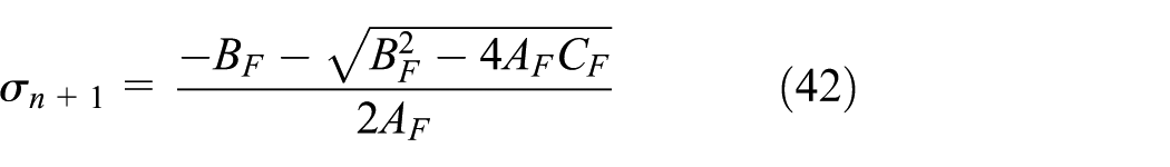
where

A_{F} = - (E_{M} - E_{A}) ε_{M} {(\frac{1 - β_{0}}{σ_{M_{f}} - σ_{M_{s}}})}^{2}

(43)

\begin{matrix} B_{F} = 1 + (\frac{1 - β_{0}}{σ_{M_{f}} - σ_{M_{s}}}) \\ {E_{A} ε_{M} + (E_{M} - E_{A}) [2 (\frac{β_{0} σ_{M_{f}} - σ_{M_{s}}}{σ_{M_{f}} - σ_{M_{s}}}) ε_{M} - ε_{n + 1}]} \end{matrix}

(44)

\begin{matrix} C_{F} = {E_{A} ε_{M} + (E_{M} - E_{A}) [(\frac{β_{0} σ_{M_{f}} - σ_{M_{s}}}{σ_{M_{f}} - σ_{M_{s}}}) ε_{M} - ε_{n + 1}]} \\ (\frac{β_{0} σ_{M_{f}} - σ_{M_{s}}}{σ_{M_{f}} - σ_{M_{s}}}) - E_{A} ε_{n + 1} - (σ_{0} - E_{0} ε_{0} + Ω_{0} β_{0}) \end{matrix}

(45)

For the martensite-austenite (reverse) transformation, the stress solution is defined by

σ_{n + 1} = \frac{- B_{R} - \sqrt{B_{R}^{2} - 4 A_{R} C_{R}}}{2 A_{R}}

(46)

where

A_{R} = (E_{M} - E_{A}) {(\frac{β_{0}}{σ_{A_{s}} - σ_{A_{f}}})}^{2} ε_{M}

(47)

\begin{matrix} B_{R} = 1 + (\frac{β_{0}}{σ_{A_{s}} - σ_{A_{f}}}) \\ {E_{A} ε_{M} - (E_{M} - E_{A}) [ε_{n + 1} + 2 (\frac{β_{0}}{σ_{A_{s}} - σ_{A_{f}}}) ε_{M}]} \end{matrix}

(48)

\begin{matrix} C_{R} = (\frac{β_{0}}{σ_{A_{s}} - σ_{A_{f}}}) \\ {- E_{A} ε_{M} + (E_{M} - E_{A}) [ε_{n + 1} - (\frac{β_{0}}{σ_{A_{s}} - σ_{A_{f}}}) ε_{M}]} \\ - E_{A} ε_{n + 1} - (σ_{0} - E_{0} ε_{0} + Ω_{0} β_{0}) \end{matrix}

(49)

Numerical simulations

SMA thermomechanical behavior is now of concern considering the assumed phase transformation kinetics. The different polynomials and the classical Brinson’s model are compared with sets of experimental data, obtained from different references, representing distinct macroscopic phenomena: temperature-induced phase transformation with constant stress; pseudoelasticity; one-way shape memory effect; two-way shape memory effect; internal subloops due to incomplete phase transformation. The characterization procedure discussed in Section 3 is employed. Since different materials were used to obtain the experimental data employed as reference for distinct macroscopic phenomena, different model parameters values are employed in the numerical simulations.

A metric is adopted to establish a numerical-experimental comparison of each model. Basically, it is assumed the following discrepancy factor for each point:

e_{i} = \frac{| P_{i}^{Num} - P_{i}^{Exp} |}{P_{i}^{Exp}}

(50)

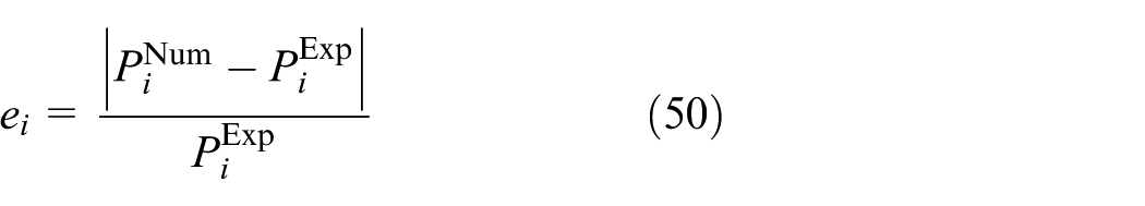
where the parameter $P_{i} = σ_{i}$ for strain-driven cases, and $P_{i} = ε_{i}$ for temperature and stress-driven cases. This allows one to define a general average discrepancy that aims to establish a quantitative comparison among the models:

e = \frac{1}{N} \sum_{i = 1}^{N} e_{i}

(51)

where N is the total number of points considered in the analysis. Note that the number of points must be equal for the experimental and numerical calculations to properly compute this metric. All the models are implemented using the Octave-Matlab.

Temperature-induced phase transformation

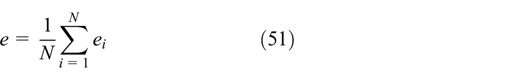
The temperature-induced phase transformation phenomenon is of concern, investigating the influence of the constant stress levels using the experimental data by Hartl et al. (2010a) as reference. The constitutive parameters are presented in Table 3, where it should be noticed that the maximum recoverable strain, $ε_{M}$ , depends on the stress level (Hartl et al., 2010b).

Table 3.

Experimental properties of the SMA reported by Hartl et al. (2010a).

$E_{A} [GPa]$	$E_{M} [GPa]$	α_A [°C⁻¹]	α_M [°C⁻¹]	$C_{A}$ [MPa/°C]
90	63	10 × 10⁻⁶	10 × 10⁻⁶	14.9
$C_{M}$ [MPa/°C]	M_s [°C]	M_f [°C]	A_s [°C]	A_f [°C]
10.6	20	−16	24	48
$σ_{s} [MPa]$	$σ_{f} [MPa]$	$ε_{M}^{(σ = 90 MPa)} [%]$	$ε_{M}^{(σ = 150 MPa)} [%]$	$ε_{M}^{(σ = 200 MPa)} [%]$
0	0	0.65	0.99	1.17

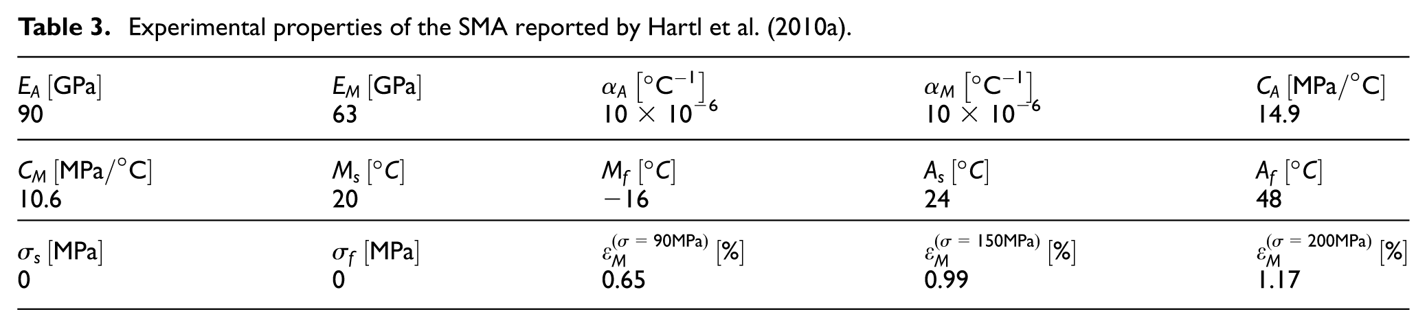
The temperature-driven case assumes prescribed temperature and constant stress, estimating strain from constitutive equations. Initially, the sample is in austenitic phase with $T > A_{f}$ , being subjected to a temperature decreases up to $T < M_{f}$ to induce phase transformations. Afterward, the temperature increases again up to the initial value. The complete temperature load cycles are presented in Figure 8.

Figure 8.

Temperature-driven loads for different constant stress levels from Hartl et al. (2010a).

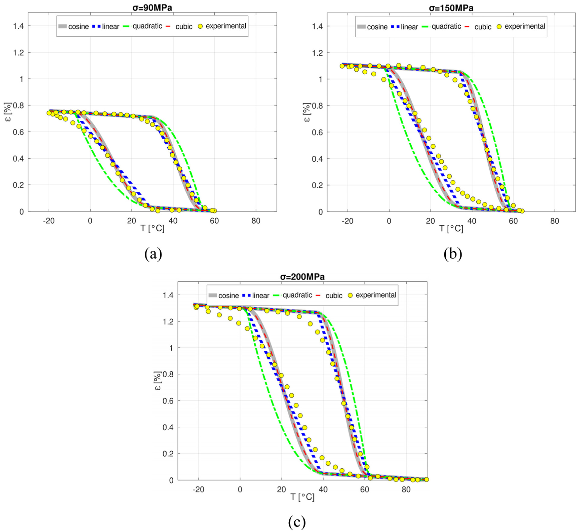
Results of the strain-temperature curves predicted by the constitutive models are presented in Figure 9, together with experimental data. Without phase transformations, the strain variation is due to the thermal expansion. Note that the strain is almost constant in the regions with $\overset{\cdot}{T} < 0$ , $T > M_{s}$ , and $T < M_{f}$ or $\overset{\cdot}{T} > 0$ , $T < A_{s}$ , and $T > A_{f}$ . It should be pointed out that all models present a good agreement with experimental data. In addition, the cubic polynomial has results close to the cosine model and the quadratic polynomial has the most discrepant behavior.

Figure 9.

Temperature-induced phase transformation compared with experimental data by Hartl et al. (2010a): (a) $σ = 90 MPa$ , (b) $σ = 150 MPa$ , and (c) $σ = 200 MPa$ .

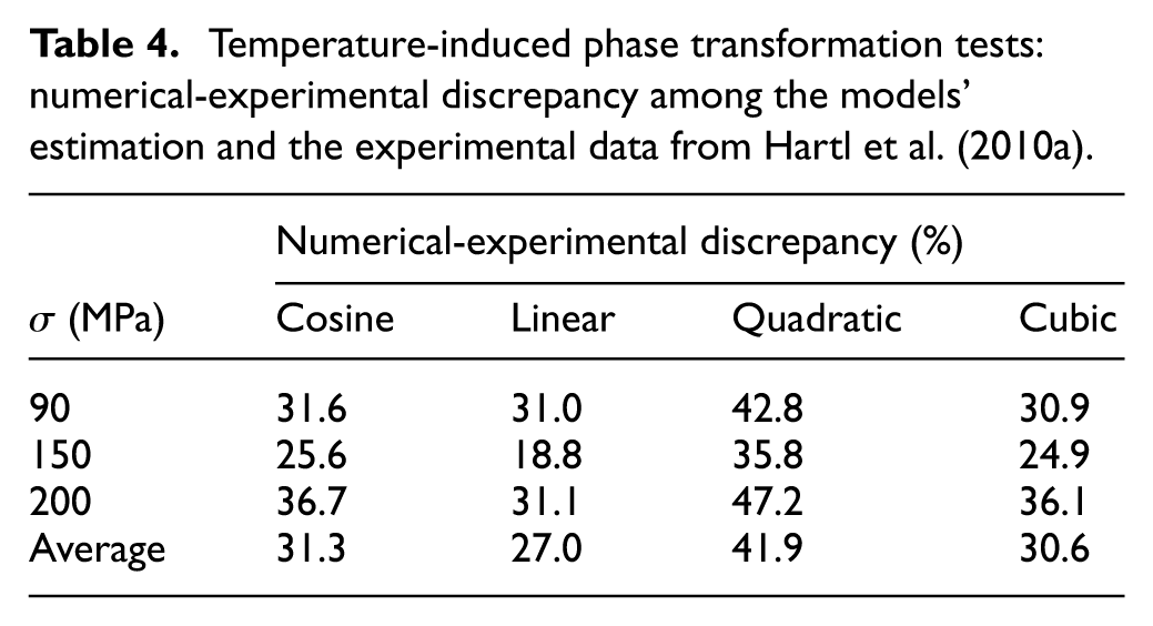
The analysis of numerical-experimental discrepancy metric is presented in Table 4. The linear function presents the smallest discrepancies in two of the three cases ( $σ = 150 MPa$ and $σ = 200 MPa$ ), with an improvement of up to 26.5% when compared with the cosine function. The quadratic polynomial presents the worst estimation for all three cases. The cubic function presents the best estimation for one case ( $σ = 90 MPa$ ), and the difference compared with the cosine is around 2% for all three values of σ.

Table 4.

Temperature-induced phase transformation tests: numerical-experimental discrepancy among the models’ estimation and the experimental data from Hartl et al. (2010a).

	Numerical-experimental discrepancy (%)
σ (MPa)	Cosine	Linear	Quadratic	Cubic
90	31.6	31.0	42.8	30.9
150	25.6	18.8	35.8	24.9
200	36.7	31.1	47.2	36.1
Average	31.3	27.0	41.9	30.6

Pseudoelasticity

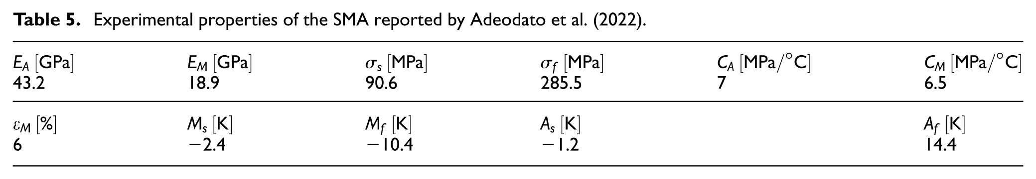
The pseudoelasticity is now investigated considering the experimental data reported by Adeodato et al. (2022) using the constitutive parameters listed in Table 5. This set of experimental data considers, for each case, a strain-driven case with a constant temperature, while the stress is computed for each model. The strain load cycle is defined by $ε = 0 % \to 10.5 % \to 0 %$ , as represented in Figure 10. Three different temperatures are evaluated: $30^{°} C$ , $50^{°} C$ , and $70^{°} C$ .

Table 5.

Experimental properties of the SMA reported by Adeodato et al. (2022).

$E_{A} [GPa]$	$E_{M} [GPa]$	$σ_{s} [MPa]$	$σ_{f} [MPa]$	$C_{A}$ [MPa/°C]	$C_{M}$ [MPa/°C]
43.2	18.9	90.6	285.5	7	6.5
$ε_{M} [%]$	$M_{s} [K]$	$M_{f} [K]$	$A_{s} [K]$		$A_{f} [K]$
6	−2.4	−10.4	−1.2		14.4

Figure 10.

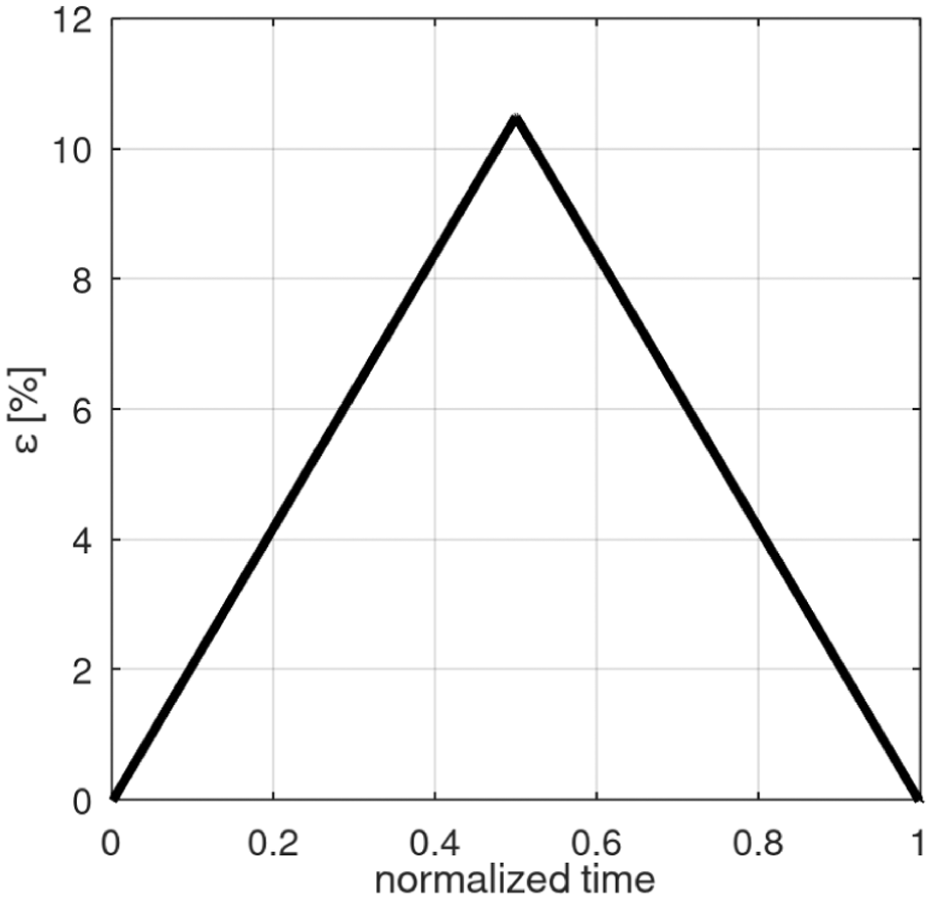
Pseudoelastic strain-driven load for $T =$ 30°C, 50°C, and 70°C from Adeodato et al. (2022).

Results of the pseudoelastic tests are presented in Figure 11 for different temperatures. Essentially, the sample is initially at austenitic phase, being subjected to a strain-driven case and a constant temperature. Note that the loading-unloading induces the austenite-martensite phase transformation and, afterward, an elastic response occurs at the martensitic phase. The subsequent unloading promotes the reverse transformation that finishes with an elastic response in austenitic phase. It should be pointed out that after the loading-unloading process, the sample is in a stress-free state being subjected to a dissipation process associated with the hysteresis loop. It is also noticeable that the increase of temperature promotes a shift of the hysteresis loop. Once again, all models present a good agreement with experimental data and the cubic polynomial is close to the cosine function.

Figure 11.

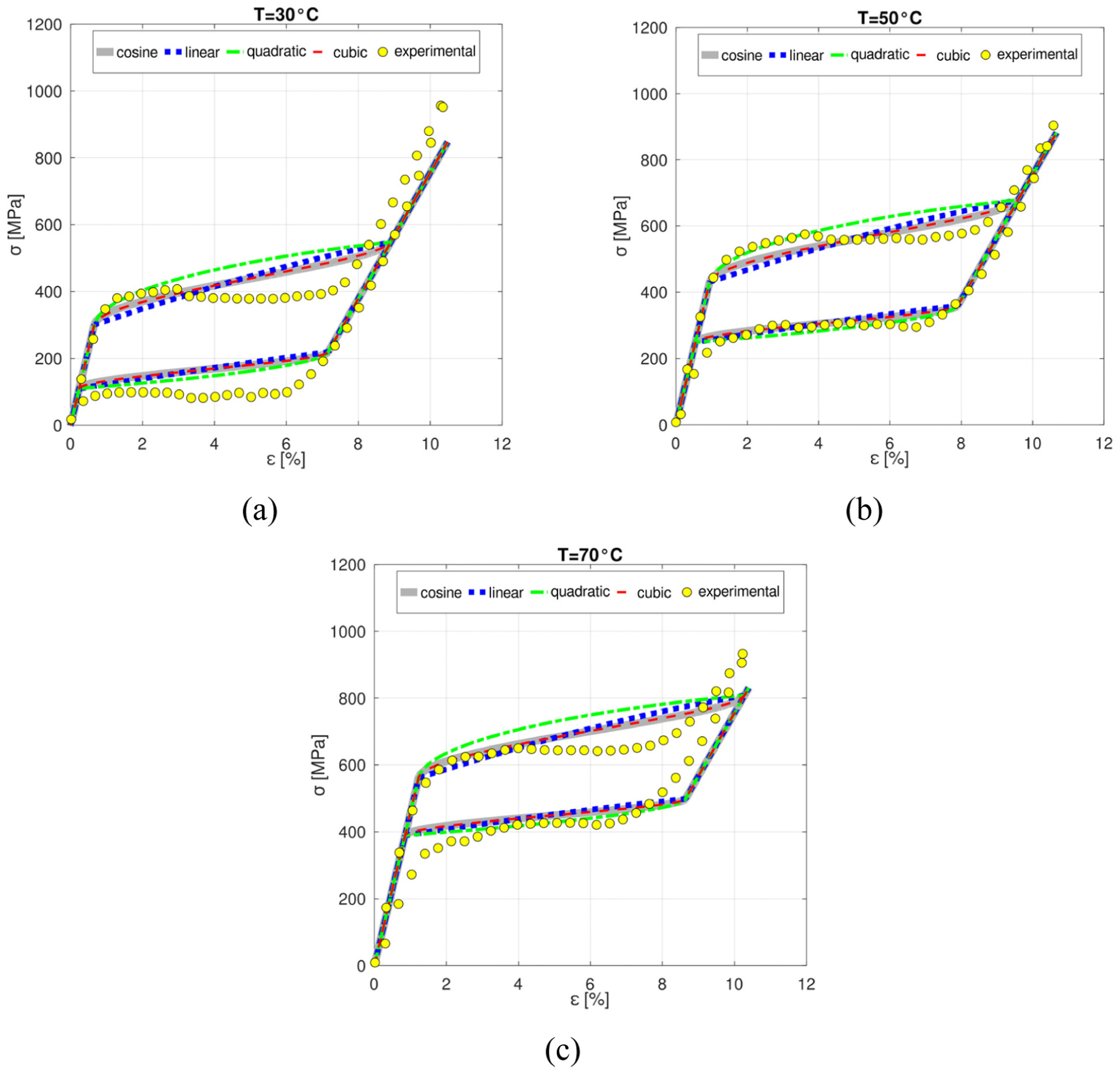
Pseudoelastic strain-driven effect compared with experimental data by Adeodato et al. (2022): (a) $T = 30^{°} C$ , (b) $T = 50^{°} C$ , and (c) $T = 70^{°} C$ .

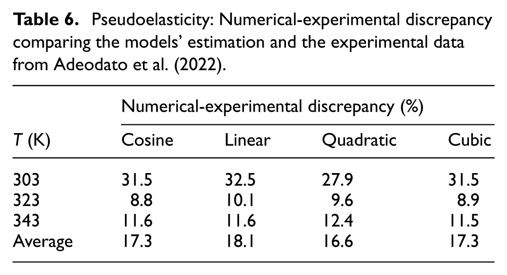
For a quantitative comparison, the numerical-experimental discrepancy is presented in Table 6. Comparing the discrepancy, the quadratic, the cubic and the cosine functions obtained the best estimation for one case. Although the linear polynomial model obtained the worst estimation for two cases, a small difference is observed when compared with the best and the worst estimations for all cases. Comparing the experimental data for all the three temperatures, the average errors are: 17.3% for the cosine, 18.1% for the linear, 16.6% for the quadratic, and 17.3% for the cubic. This result indicates that the models have very close estimations, the difference between the worst (linear) and the best (quadratic) for these data is only 1.5%. Another point that should be evaluated is the computational cost. The linear polynomial model is approximately 87% faster than the other functions due to the analytical solution, while all the other functions demand iterative solutions.

Table 6.

Pseudoelasticity: Numerical-experimental discrepancy comparing the models’ estimation and the experimental data from Adeodato et al. (2022).

	Numerical-experimental discrepancy (%)
T (K)	Cosine	Linear	Quadratic	Cubic
303	31.5	32.5	27.9	31.5
323	8.8	10.1	9.6	8.9
343	11.6	11.6	12.4	11.5
Average	17.3	18.1	16.6	17.3

Shape memory effect

Shape memory effect is now of concern considering two different phenomena: one-way shape memory effect (SME) using experimental data by Adeodato et al. (2022) as reference; two-way shape memory effect (TWSME) using experimental data by Luo and Abel (2007) as reference.

Initially, the SME is of concern, and constitutive parameters presented in Table 5 are used. Typically, a mechanical loading is applied at a temperature lower than $M_{f}$ ; in this case, $M_{f} = - 10 . 4^{°} C$ , and $T = - 30^{°} C$ . The complete load cycle is split into two parts, as represented in Figure 12: first, a mechanical loading-unloading process is applied, keeping $\overset{\cdot}{T} = 0$ to obtain the reorientation from twinned to detwinned martensite and resulting in a residual strain; next, $\overset{\cdot}{σ} = 0$ and the temperature is increased to a value higher than $A_{f}$ to obtain the austenitic transformation, followed by a decreasing up to $- 30^{°} C$ , where the microstructure is twinned martensite again.

Figure 12.

Shape memory effect load cycle for the SME based on Adeodato et al. (2022): (a) stress and (b) temperature.

It should be pointed out that the experimental data deal only with the martensite reorientation during the mechanical loading-unloading process, and therefore, do not consider the subsequent thermal load responsible for the shape recovery. Nevertheless, the temperature variation is simulated to demonstrate the model ability to represent the shape recovery represented by the transformation from detwinned martensite to austenite when $\overset{\cdot}{T} > 0$ . On this basis, experimental-numerical comparison is restricted to the mechanical load. Figure 13 presents the SME simulations split into two parts: martensitic reorientation due to mechanical load (Figure 13(a)); shape recovery due to temperature variation (Figure 13(b)). It is noticeable that all models capture the general behavior. A similar trend is observed for both stress-driven and temperature-driven cases: the cosine and cubic functions are very close, the linear function crosses the cubic and cosine functions halfway through the transformation, and the quadratic function has the most discrepant behavior.

Figure 13.

Shape memory effect: (a) martensitic reorientation induced by the mechanical load establishing a comparison with the experimental data from Adeodato et al. (2022) and (b) shape recovery induced by the thermal load.

Two-way shape memory effect (TWSME) is now of concern. Experimental tests due to Luo and Abel (2007) are used as reference. The original reference presented just the temperatures for start and finish of phase transformation, being measured before the samples training. Table 7 are employed as material properties including adjusted values and other taken from Hartl et al. (2010a).

Table 7.

Material properties for the TWSME based on the data reported by Luo and Abel (2007).

$E_{A} [GPa]$ ^a	$E_{M} [GPa]$ ^a	α_A = α_M [°C⁻¹]^a
90	63	10×10⁻⁶
$M_{f}$ [°C]^b	$M_{s}$ [°C]^b	$A_{s}$ [°C]^b	$A_{f}$ [°C]^b
50	63	65	76
$ε_{M} [%]$ ^c	$C_{A} = C_{M}$ [MPa/°C]^c	$σ_{s} = σ_{f} [MPa]$ ^c	$σ_{TW} [MPa]$ ^c
2.88	15	0	250

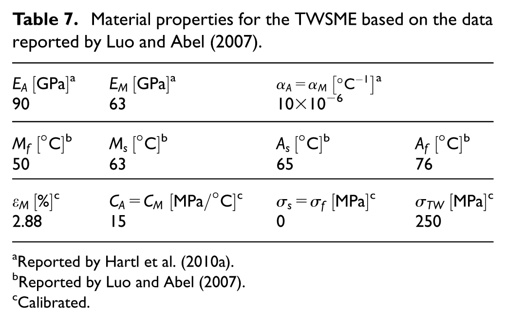
Reported by Hartl et al. (2010a).

Reported by Luo and Abel (2007).

Calibrated.

TWSME is treated as a temperature-driven case, shown in Figure 14. Figure 15 presents numerical simulations as strain-temperature curves. It is noticeable that shape changes occur due to temperature variations, without mechanical loads. This behavior is the essence of the TWSME, different of the SME that needs a mechanical load to induce shape change. 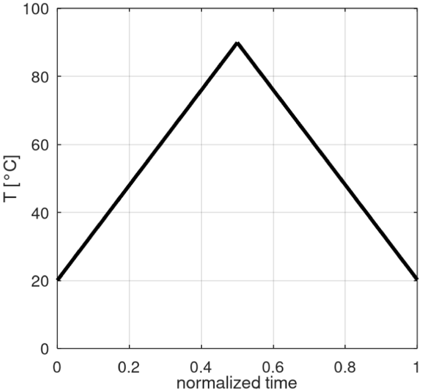This effect is only possible due to a previous training process that induces a residual stress field, represented by $σ_{TW}$ in the model. All models capture the qualitative behavior but, the linear polynomial estimation tends to be closer to the cosine and cubic functions.

Figure 14.

Temperature-driven for the two-way shape memory effect from Luo and Abel (2007).

Figure 15.

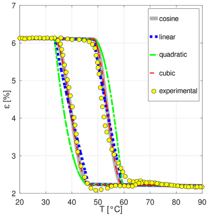
Two-way shape memory effect compared with experimental data from Luo and Abel (2007).

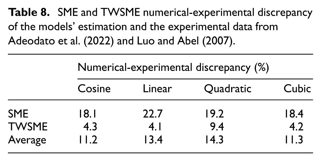
Results of the numerical-experimental discrepancy are presented in Table 8. The linear function obtained the highest value for the SME and the smallest for the TWSME. Considering both one-way and two-way, the average discrepancies are: 11.2% for the cosine, 13.4% for the linear, 14.3% for the quadratic, and 11.3% for the cubic. Now, the difference between the model with the best estimations (cosine) and the model with the worst estimation (quadratic) is 2.3%.

Table 8.

SME and TWSME numerical-experimental discrepancy of the models’ estimation and the experimental data from Adeodato et al. (2022) and Luo and Abel (2007).

	Numerical-experimental discrepancy (%)
	Cosine	Linear	Quadratic	Cubic
SME	18.1	22.7	19.2	18.4
TWSME	4.3	4.1	9.4	4.2
Average	11.2	13.4	14.3	11.3

Internal subloops

This section investigates internal subloops associated with incomplete phase transformations. Experimental data considering material properties characterized in Section 3 and presented in Table 2 are employed, being based on tests reported by Alvares et al. (2024). Different strain-driven load cycles are of concern in order to show different aspects of complex SMA thermomechanical responses. All tests are performed at a constant temperature $T = 30^{°} C$ .

Figure 16 considers a mechanical loading process, named load I. The stress-strain curves of this response are presented in Figure 17 showing internal subloops due to incomplete phase transformation. It is noticeable that the constitutive models present good agreement with experimental data.

Figure 16.

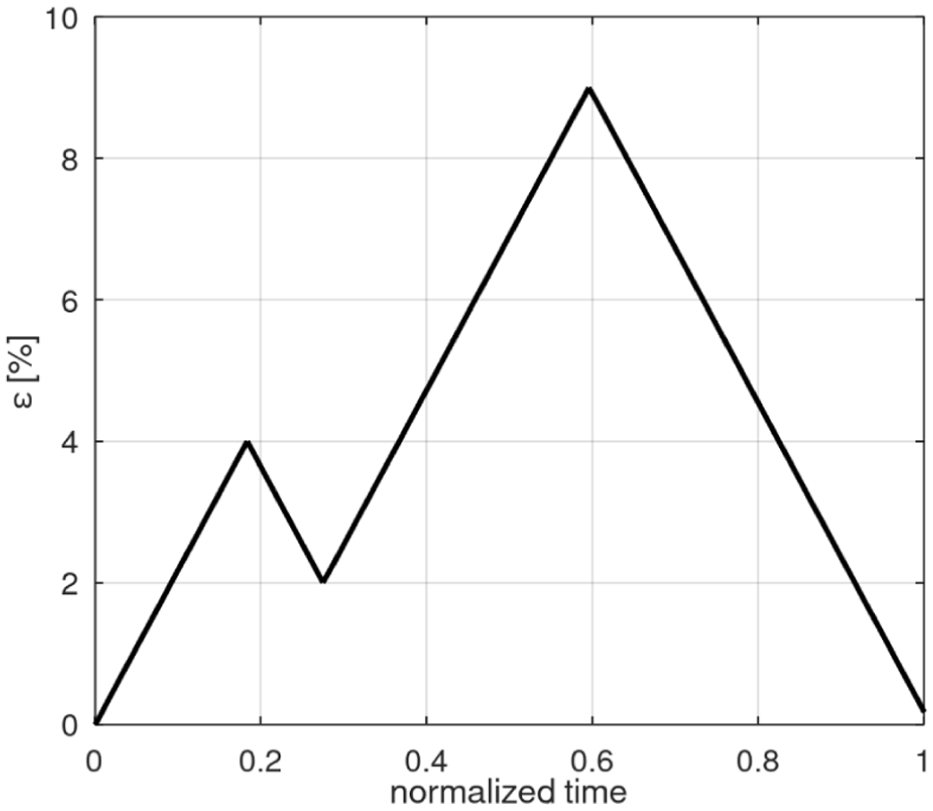
Strain-driven load I based on experimental tests by Alvares et al. (2024).

Figure 17.

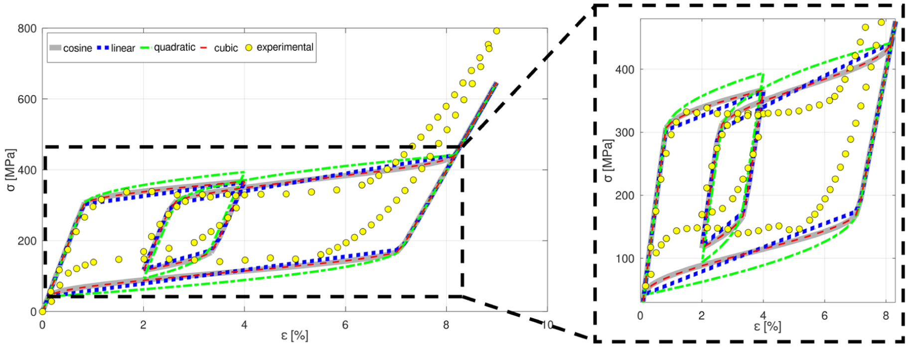
Pseudoelastic internal subloops based on experimental tests by Alvares et al. (2024), load I.

A different strain-driven load (load II) is now of concern, being presented in Figure 18. Figure 19 presents the stress-strain curves showing again internal subloops. Once again, all models present a good agreement.

Figure 18.

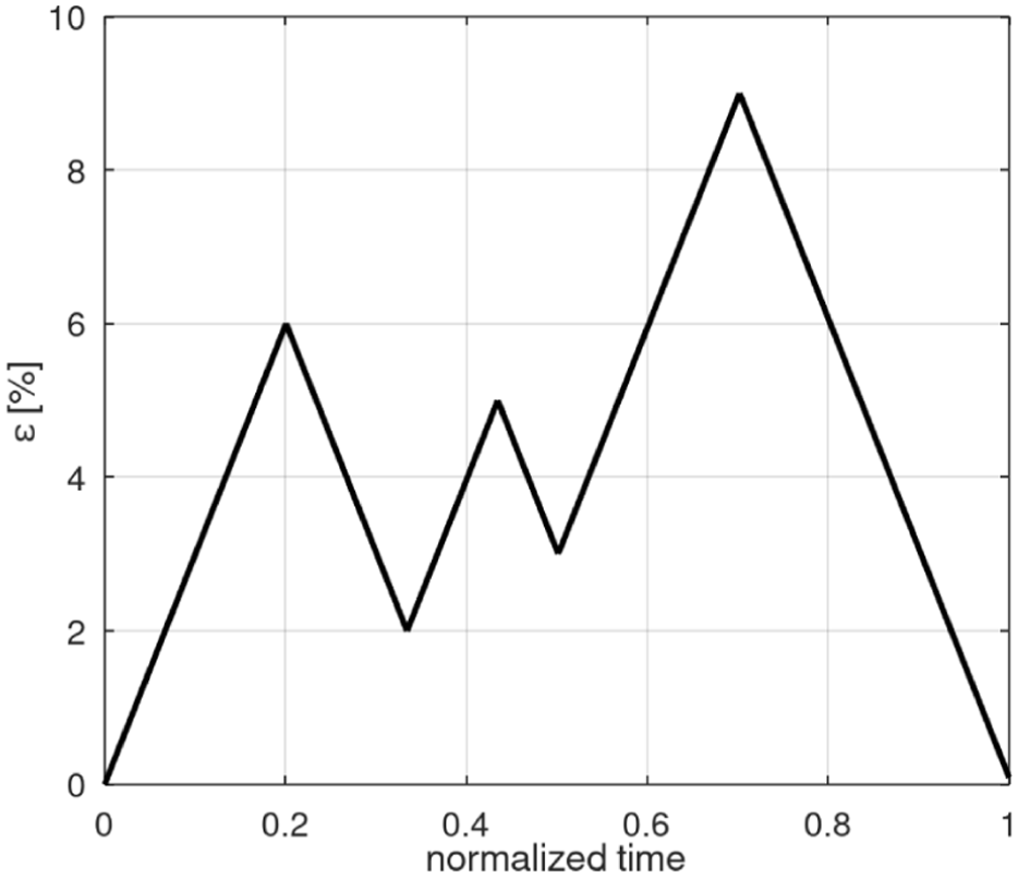
Strain-driven load II based on experimental tests by Alvares et al. (2024).

Figure 19.

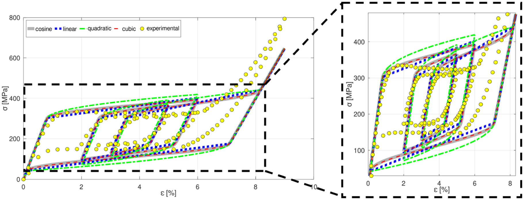
Pseudoelastic internal subloops based on experimental tests by Alvares et al. (2024), load II.

Finally, a different strain-driven load is employed (load III), being presented in Figure 20, while the stress-strain response shown in Figure 21, that depicts details about different cycles. Although all models present a reasonable agreement, it is noticeable that the cosine and cubic functions are overlapped, while the quadratic function has the most discrepant trend.

Figure 20.

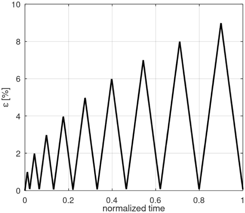
Strain-driven load III based on experimental tests by Alvares et al. (2024).

Figure 21.

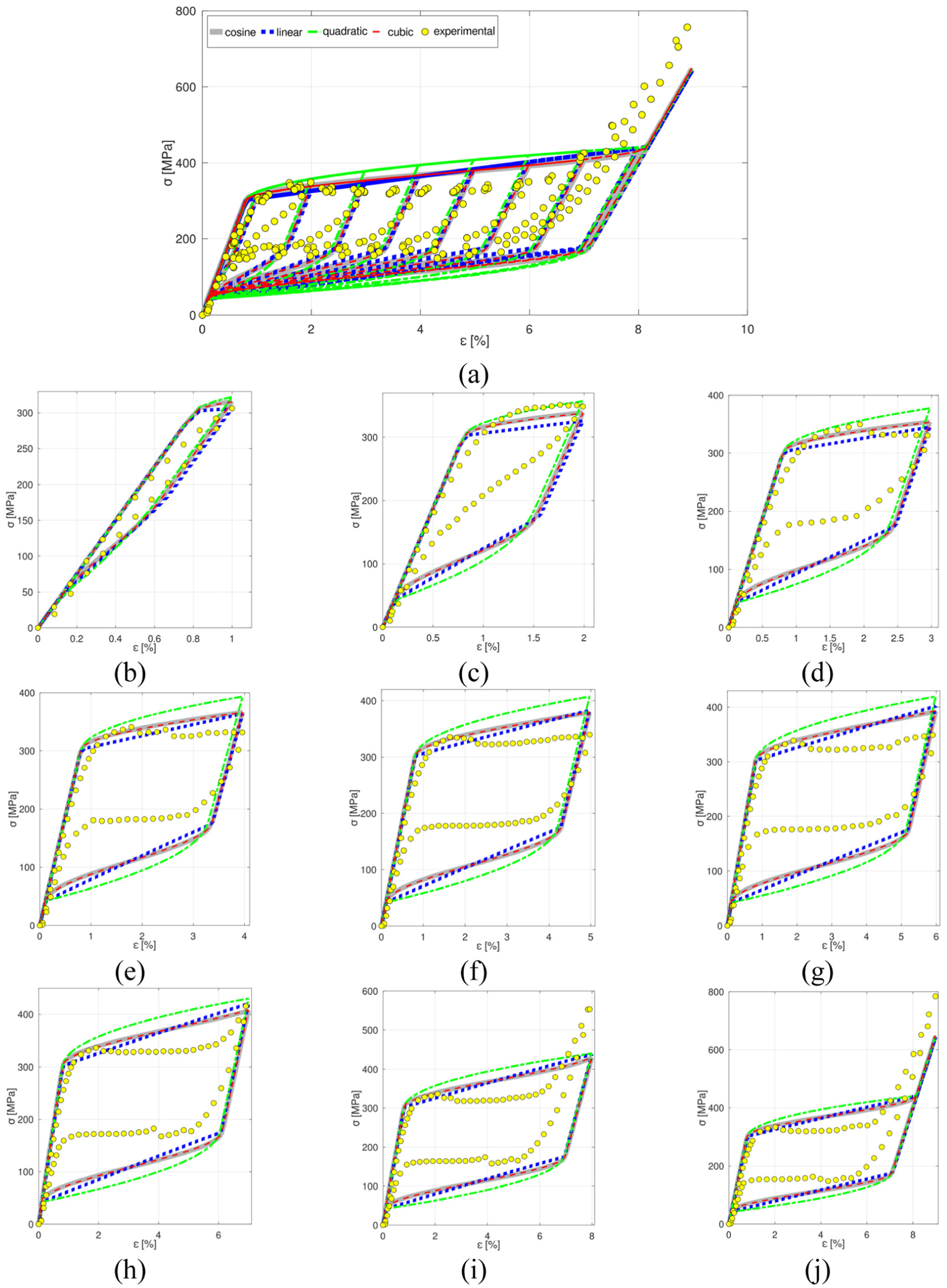
Pseudoelastic internal subloops based on experimental tests by Alvares et al. (2024), load III: (a) complete load history; (b) $ε = 0 % \to 1 % \to 0 %$ , (c) $ε = 0 % \to 2 % \to 0 %$ , (d) $ε = 0 % \to 3 % \to 0 %$ , (e) $ε = 0 % \to 4 % \to 0 %$ , (f) $ε = 0 % \to 5 % \to 0 %$ , (g) $ε = 0 % \to 6 % \to 0 %$ , (h) $ε = 0 % \to 7 % \to 0 %$ , (i) $ε = 0 % \to 8 % \to 0 %$ , and (j) $ε = 0 % \to 9 % \to 0 %$ .

The computational efficiency of the linear function also must be highlighted when compared with the other functions which the analytical solutions are not available. In general, linear polynomial simulations are 86% faster than the others since it does not need the iterative process.

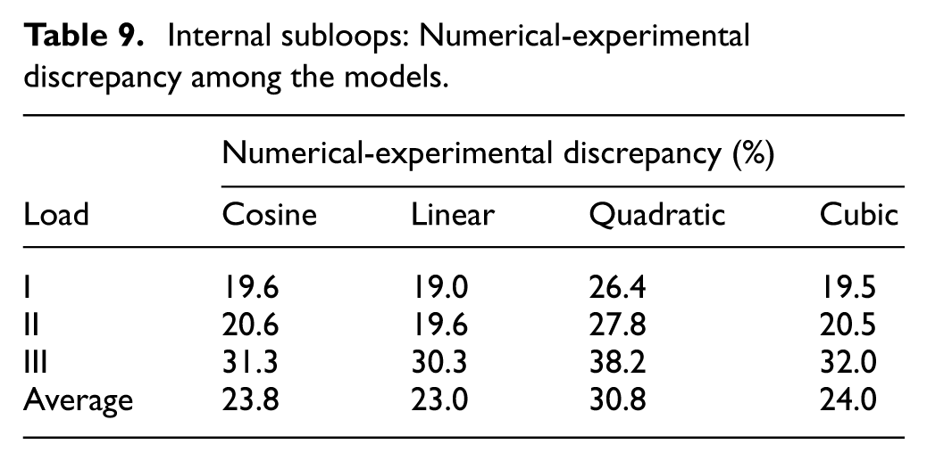
The quantitative numerical-experimental discrepancies are listed in Table 9. It should be noted that the linear function has the best estimation for all the load cases, with results compared with the cosine and quadratic functions.

Table 9.

Internal subloops: Numerical-experimental discrepancy among the models.

	Numerical-experimental discrepancy (%)
Load	Cosine	Linear	Quadratic	Cubic
I	19.6	19.0	26.4	19.5
II	20.6	19.6	27.8	20.5
III	31.3	30.3	38.2	32.0
Average	23.8	23.0	30.8	24.0

Conclusions

This paper deals with SMA constitutive model with assumed phase transformation kinetics, investigating the use of polynomial functions. The classical Brinson’s model is employed as the essential framework, but novel ideas are incorporated to deal with tensile-compressive behaviors and two-way shape memory effect.

Polynomial phase transformation kinetics are derived, considering linear, quadratic, and cubic functions. Numerical procedure has a direct implementation for stress-driven and temperature-driven cases. The strain-driven case needs an iterative procedure, but analytical solutions can be derived for the linear polynomials, which is an attractive advantage since it results in a considerably less computational cost.

Numerical simulations are carried out to show the model ability to deal with the SMA thermomechanical behavior. Essentially, the following cases are treated: temperature-induced phase transformation with constant stress; pseudoelasticity; one-way shape memory effect; two-way shape memory effect; internal subloops due to incomplete phase transformation. Considering all these sets of experimental data, 11 different load scenarios are evaluated. All models present a good match with experimental data, being able to capture the general SMA thermomechanical behavior.

Results highlight that the use of the linear function to describe the phase kinetics transformation is a good alternative, improving the computational efficiency without loss the capability to describe the complex behavior of SMAs. In general, linear polynomial simulations are 86% faster than the others since it does not need the iterative process.

Footnotes

Appendix 1

This appendix aims to derive the closed-form analytical expressions for strain-driven loads using linear polynomial phase transformation model, as presented in Section 4. By considering the pseudoelastic phenomenon, $\overset{\cdot}{T} = 0$ , $β_{T} = 0$ , and ${\overset{\cdot}{β}}_{T} = 0$ , which implies that $β = β_{σ}$ Hence, the constitutive model is defined by

(A.1)

σ_{n + 1} = E_{n + 1} ε_{n + 1} - Ω_{n + 1} β_{n + 1} + (σ_{0} - E_{0} ε_{0} + Ω_{0} β_{0})

Since $Ω = E ε_{M}$ and $E = E_{A} + β (E_{M} - E_{A})$ , equation (A.1) can be manipulated to obtain the following expression

(A.2)

\begin{matrix} σ_{n + 1} + [E_{A} ε_{M} - (E_{M} - E_{A}) ε_{n + 1}] β_{n + 1} + (E_{M} - E_{A}) \\ ε_{M} β_{n + 1}^{2} - E_{A} ε_{n + 1} - (σ_{0} - E_{0} ε_{0} + Ω_{0} β_{0}) = 0 \end{matrix}

The strain-driven case assumes $ε_{n + 1} = ε_{n} + Δ ε$ , which is known; on the other hand, $σ_{n + 1}$ and $β_{n + 1}$ are unknows. Additionally, $β_{n + 1} = {(β_{σ})}_{n + 1}$ and $β_{0} = β_{σ_{0}}$ .

Using equations (8) and (22), the martensite volume fraction for the austenite-martensite transformation is

(A.3)

β_{n + 1} = (\frac{1 - β_{0}}{σ_{M_{f}} - σ_{M_{s}}}) σ_{n + 1} + (\frac{β_{0} σ_{M_{f}} - σ_{M_{s}}}{σ_{M_{f}} - σ_{M_{s}}})

Replacing equation (A.3) into equation (A.2)

(A.4)

\begin{matrix} σ_{n + 1} + [E_{A} ε_{M} - (E_{M} - E_{A}) ε_{n + 1}] [(\frac{1 - β_{0}}{σ_{M_{f}} - σ_{M_{s}}}) σ_{n + 1} + (\frac{β_{0} σ_{M_{f}} - σ_{M_{s}}}{σ_{M_{f}} - σ_{M_{s}}})] + (E_{M} - E_{A}) ε_{M} \\ [{(\frac{1 - β_{0}}{σ_{M_{f}} - σ_{M_{s}}})}^{2} σ_{n + 1}^{2} + {(\frac{β_{0} σ_{M_{f}} - σ_{M_{s}}}{σ_{M_{f}} - σ_{M_{s}}})}^{2} + 2 (\frac{1 - β_{0}}{σ_{M_{f}} - σ_{M_{s}}}) (\frac{β_{0} σ_{M_{f}} - σ_{M_{s}}}{σ_{M_{f}} - σ_{M_{s}}}) σ_{n + 1}] \\ - E_{A} ε_{n + 1} - (σ_{0} - E_{0} ε_{0} + Ω_{0} β_{0}) = 0 \end{matrix}

Realizing that equation (A.4) is a quadratic polynomial function of $σ_{n + 1}$ , its compact form is written as

(A.5)

A_{F} σ_{n + 1}^{2} + B_{F} σ_{n + 1} + C_{F} = 0

where

(A.6)

A_{F} = (E_{M} - E_{A}) ε_{M} {(\frac{1 - β_{0}}{σ_{M_{f}} - σ_{M_{s}}})}^{2}

(A.7)

B_{F} = 1 + (\frac{1 - β_{0}}{σ_{M_{f}} - σ_{M_{s}}}) {E_{A} ε_{M} + (E_{M} - E_{A}) [2 (\frac{β_{0} σ_{M_{f}} - σ_{M_{s}}}{σ_{M_{f}} - σ_{M_{s}}}) ε_{M} - ε_{n + 1}]}

(A.8)

C_{F} = {E_{A} ε_{M} + (E_{M} - E_{A}) [(\frac{β_{0} σ_{M_{f}} - σ_{M_{s}}}{σ_{M_{f}} - σ_{M_{s}}}) ε_{M} - ε_{n + 1}]} (\frac{β_{0} σ_{M_{f}} - σ_{M_{s}}}{σ_{M_{f}} - σ_{M_{s}}}) - E_{A} ε_{n + 1} - (σ_{0} - E_{0} ε_{0} + Ω_{0} β_{0})

Consequently, the solutions of equation (A.5) are

(A.9)

σ_{n + 1} = \frac{- B_{F} \pm \sqrt{B_{F}^{2} - 4 A_{F} C_{F}}}{2 A_{F}}

The solution of $σ_{n + 1}$ for the transformation from austenite to martensite has the bounds $σ_{M_{s}} \leq σ_{n + 1} \leq σ_{M_{f}}$ . In a general sense, both solutions should be evaluated to verify which one satisfy this limit requirement. For all the cases simulated in this study, the solution is $- B_{F} - \sqrt{B_{F}^{2} - 4 A_{F} C_{F}} / 2 A_{F}$ , as defined in equation (42).

On the other hand, the volume fraction for the martensite-austenite transformation is calculated by manipulating equations (10) and (24), obtained the following relation

(A.10)

β_{n + 1} = (\frac{β_{0}}{σ_{A_{s}} - σ_{A_{f}}}) σ_{n + 1} - (\frac{β_{0}}{σ_{A_{s}} - σ_{A_{f}}})

Replacing equation (A.10) into equation (A.2)

(A.11)

\begin{matrix} σ_{n + 1} + [E_{A} ε_{M} - (E_{M} - E_{A}) ε_{n + 1}] [(\frac{β_{0}}{σ_{A_{s}} - σ_{A_{f}}}) σ_{n + 1} - (\frac{β_{0}}{σ_{A_{s}} - σ_{A_{f}}})] + (E_{M} - E_{A}) {(\frac{β_{0}}{σ_{A_{s}} - σ_{A_{f}}})}^{2} ε_{M} \\ [σ_{n + 1}^{2} - 1 - 2 σ_{n + 1}] - E_{A} ε_{n + 1} - (σ_{0} - E_{0} ε_{0} + Ω_{0} β_{0}) = 0 \end{matrix}

The compact form of the quadratic expressions defined in equation (A.11) is

(A.12)

A_{R} σ_{n + 1}^{2} + B_{R} σ_{n + 1} + C_{R} = 0

where

(A.13)

A_{R} = (E_{M} - E_{A}) {(\frac{β_{0}}{σ_{A_{s}} - σ_{A_{f}}})}^{2} ε_{M}

(A.14)

\begin{matrix} B_{R} = 1 + (\frac{β_{0}}{σ_{A_{s}} - σ_{A_{f}}}) \\ {E_{A} ε_{M} - (E_{M} - E_{A}) [ε_{n + 1} + 2 (\frac{β_{0}}{σ_{A_{s}} - σ_{A_{f}}}) ε_{M}]} \end{matrix}

(A.15)

\begin{matrix} C_{R} = (\frac{β_{0}}{σ_{A_{s}} - σ_{A_{f}}}) \\ {- E_{A} ε_{M} + (E_{M} - E_{A}) [ε_{n + 1} - (\frac{β_{0}}{σ_{A_{s}} - σ_{A_{f}}}) ε_{M}]} \\ - E_{A} ε_{n + 1} - (σ_{0} - E_{0} ε_{0} + Ω_{0} β_{0}) \end{matrix}

At last, the solutions of equation (A.12) are written as

(A.16)

σ_{n + 1} = \frac{- B_{R} \pm \sqrt{B_{R}^{2} - 4 A_{R} C_{R}}}{2 A_{R}}

The two solutions from equation (A.16) should be evaluated considering that $σ_{A_{s}} \geq σ_{n + 1} \geq σ_{A_{f}}$ for the martensite-austenite transformation. Again, for all the cases simulated in this study, the solution is $- B_{R} - \sqrt{B_{R}^{2} - 4 A_{R} C_{R}} / 2 A_{R}$ , as defined in equation (46).

ORCID iDs

Lucas L. Vignoli

Marcelo A. Savi

Pedro Manuel Calas Lopes Pacheco

Funding

The authors disclosed receipt of the following financial support for the research, authorship, and/or publication of this article: The authors would like to acknowledge the support of the Brazilian Research Agencies CNPq (Conselho Nacional de Desenvolvimento Científico e Tecnológico), CAPES (Coordenação de Aperfeiçoamento de Pessoal de Nível Superior), and FAPERJ (Fundação Carlos Chagas Filho de Amparo à Pesquisa do Estado do Rio de Janeiro) and through the INCT-EIE (National Institute of Science and Technology - Smart Structures in Engineering), and FAPEMIG (Fundação de Amparo à Pesquisa do Estado de Minas Gerais). The support of the AFOSR (Air Force Office of Scientific Research) (FA9550-23-4301-0527) is also acknowledged.

Declaration of conflicting interests

The authors declared no potential conflicts of interest with respect to the research, authorship, and/or publication of this article.

Data availability statement

The datasets generated during and/or analyzed during the current study are available from the corresponding author upon reasonable request.*

References

Adeodato

Duarte

Monteiro

LLS

, et al. (2021) Synergistic use of piezoelectric and shape memory alloy elements for vibration-based energy harvesting. International Journal of Mechanical Sciences 194: 106206.

Adeodato

Vignoli

Paiva

, et al. (2022) A shape memory alloy constitutive model with polynomial phase transformation kinetics. Shape Memory and Superelasticity 8: 277–294.

Alvares

Dornelas

Oliveira

, et al. (2024) Thermomechanical description of shape memory alloys using the preisach model. Smart Materials and Structures 33: 035019.

Auricchio

Sacco

(1997) A one-dimensional model for superelastic shape-memory alloys with different elastic properties between austenite and martensite. International Journal of Non-Linear Mechanics 32: 1101–1114.

Boyd

Lagoudas

(1994) Constitutive model for simultaneous transformation and reorientation in shape memory alloys. In: Brinson

Moran

(eds) Mechanics of Phase Transformation and Shape Memory Alloys. ASME, pp. 159–177.

Boyd

Lagoudas

(1996) A thermodynamical constitutive model for shape memory materials. Part I. The monolithic shape memory alloy. International Journal of Plasticity 12: 805–842.

Brack

Ghasemnejad

(2025) Effect of embedded shape memory alloy (SMA) on the low-velocity impact behaviour of stringer stiffened composite plates. Applied Composite Materials 32: 21–44.

Brinson

(1993) One-dimensional constitutive behavior of shape memory alloys: Thermomechanical derivation with non-constant material functions and redefined martensite internal variable. Journal of Intelligent Material Systems and Structures 4: 229–242.

Chaudhary

Haribhakta

Jadhav

(2024) A review of shape memory alloys in MEMS devices and biomedical applications. Materials Today Proceedings. https://doi.org/10.1016/j.matpr.2024.04.105

10.

Chowdhury

(2018) Frontiers of theoretical research on shape memory alloys: A general overview. Shape Memory and Superelasticity 4(1): 26–40.

11.

Cisse

Zaki

Ben Zineb

(2016a) A review of constitutive models and modeling techniques for shape memory alloys. International Journal of Plasticity 76: 244–284.

12.

Cisse

Zaki

Zineb

(2016b) A review of modeling techniques for advanced effects in shape memory alloy behavior. Smart Materials and Structures 25: 103001.

13.

Dalave

Joseph

Patil

, et al. (2024) Meta-structures for energy absorption: Materials, designs, and applications in additive manufacturing and its future scope. Journal of the Brazilian Society of Mechanical Sciences and Engineering 46: 518.

14.

Debossan

AJD

Vignoli

(2022) Improving composite low velocity impact performance using SMA: A multiscale analysis. Mechanics Research Communications 125: 103996.

15.

Del Core

Attolico

Moramarco

, et al. (2025) Shape memory alloys for reversible restoration of ancient monuments. Shape Memory and Superelasticity 11: 44–65.

16.

Dornelas

Oliveira

Savi

, et al. (2021) Fatigue on shape memory alloys: experimental observations and constitutive modeling. International Journal of Solids and Structures 213: 1–24.

17.

Dornelas

Oliveira

Savi

(2025) A prismatic approach to describe the hysteretic behavior of smart materials: An application to shape memory alloys. Journal of Intelligent Material Systems and Structures 36(9): 563–578.

18.

Dornelas

Oliveira

Savi

(2026) Multiphysics description of smart materials using a prismatic data-driven approach. International Journal of Mechanical Sciences 311: 111180.

19.

Fang

(2022) SMAs for infrastructures in seismic zones: A critical review of latest trends and future needs. Journal of Building Engineering 57: 104918.

20.

Fonseca

Rodrigues

Savi

(2022) An overview of the mechanical description of origami-inspired systems and structures. International Journal of Mechanical Sciences 223: 107316.

21.

Fremond

(1987) Matériaux à mémoire de forme. Comptes Rendus des séances l’Academie des Sciences, Paris, Tome 304(7): 239–244.

22.

Gantz

Stroud

Fuller

, et al. (2022) Aerospace, energy recovery, and medical applications: Shape memory alloy case studies for CASMART 3rd student design challenge. Shape Memory and Superelasticity 8: 150–167.

23.

Hakimi

Ashrafi

(2023) constitutive modeling for the training process of two-way shape memory effect under thermal cyclic loading. Journal of Intelligent Material Systems and Structures 34: 1511–1526.

24.

Hartl

Lagoudas

(2007) Aerospace applications of shape memory alloys. Proceedings of the Institution of Mechanical Engineers Part G Journal of Aerospace Engineering 221: 535–552.

25.

Hartl

Lagoudas

Calkins

, et al. (2010a) Use of a Ni60Ti shape memory alloy for active jet engine chevron application: I. Thermomechanical characterization. Smart Materials and Structures 19: 015020.

26.

Hartl

Mooney

Lagoudas

, et al. (2010b) Use of a Ni60Ti shape memory alloy for active jet engine chevron application: II. Experimentally validated numerical analysis. Smart Materials and Structures 19: 015021.

27.

Dong

Nie

, et al. (2023) Comprehensive shape memory alloys constitutive models for engineering application. Materials & Design 225: 111563.

28.

Honrao

Benafan

Lawson

(2023) Data-driven study of shape memory behavior of multi-component Ni–Ti alloys in large compositional and processing space. Shape Memory and Superelasticity 9: 144–155.

29.

Ivshin

Pence

(1994) A constitutive model for hysteretic phase transition behavior. International Journal of Engineering Science 32: 681–704.

30.

Jani

Leary

Subic

, et al. (2014) A review of shape memory alloy research, applications and opportunities. Materials & Design 56: 1078–1113.

31.

Jin

Zang

Xing

, et al. (2024) Resonant peak reduction of a rotor system based on gradually variable stiffness of supports with shape memory alloy springs. Journal of Sound and Vibration 591: 118626.

32.

Sun

Wang

, et al. (2022) Optimization of aero-engine pipeline for avoiding vibration based on length adjustment of straight-line segment. Frontiers in Mechanical Engineering 17: 11.

33.

Khandelwal

Buravalla

(2009) Models for shape memory alloy behavior: An overview of modeling approaches. The International Journal of Structural Changes in Solids 1: 111–148.

34.

Kim

M-S

Heo

J-K

Rodrigue

, et al. (2023) Shape memory alloy (SMA) actuators: The role of material, form, and scaling effects. Advanced Materials 35: 2208517.

35.

Koupaei

Hosseini

SMM

Ghaini

FMM

(2016) A new optimization algorithm based on chaotic maps and golden section search method. Engineering Applications of Artificial Intelligence 50: 201–214.

36.

Kumar

Patel

Panda

, et al. (2024) A comprehensive exploration of shape memory alloys: Fundamentals, structural reinforcements, nano-analysis, machine learning perspective, and emerging applications. Mechanics of Advanced Materials and Structures 31: 11450–11483.

37.

Lagoudas

(2008) Shape Memory Alloys, Modeling and Engineering Applications. Springer.

38.

Leal

PBC

Savi

(2018) Shape memory alloy-based mechanism for aeronautical application: Theory, optimization and experiment. Aerospace Science and Technology 76: 155–163.

39.

Lemaitre

Chaboche

(1990) Mechanics of Solid Materials. Cambridge University Press.

40.

Liang

Rogers

(1990) One-dimensional thermomechanical constitutive relations for shape memory materials. Journal of Intelligent Material Systems and Structures 1: 207–234.

41.

Wang

Chen

, et al. (2025) Arresting fatigue cracks in steel plates using prestressed bonded Fe-SMA strips: Analytical prediction and experimental validation. Thin-Walled Structures 210: 112971.

42.

Liu

Dong

(2024) A constitutive model of nanoporous NiTi shape memory alloys considering tensile-compressive asymmetry, grain size and porosity. International Journal of Non-Linear Mechanics 160: 104661.

43.

Liu

Chen

Lin

, et al. (2024a) A new constitutive model of shape memory alloy and its seismic mitigation capacity compared with existing models. Advances in Structural Engineering 27: 835–853.

44.

Liu

Xiang

Pan

, et al. (2024b) Porous shape memory niti-entangled material with incredible recoverable strain for downhole sand control in oil/gas production. Applied Materials Today 38: 102249.

45.

Liu

(2021) Design and experiment of piezoelectric-shape memory alloy composite shock absorber. Materials Letters 304: 130538.

46.

Luo

Abel

(2007) A comparison of methods for the training of NiTi two-way shape memory alloy. Smart Materials and Structures 16: 2543–2549.

47.

Machado

Savi

(2003) Medical applications of shape memory alloys. Brazilian Journal of Medical and Biological Research 36(6): 683–691.

48.

Mayergoyz

(2003) Mathematical Models of Hysteresis and Their Applications. Academic Press.

49.

Medina

Herrera

Beltran

(2023) Constitutive model for superelastic shape memory alloys considering strength and stiffness degradation and residual strain: An empirical approach for engineering applications. Engineering Structures 283: 115810.

50.

Nozaki

Miyata

Hara

, et al. (2021) A robust control system against temperature variance for space-use SMA actuators. In: AIAA 2021-1561. AIAA scitech 2021 forum.

51.

Oliveira

Dornelas

Savi

, et al. (2018) A phenomenological description of shape memory alloy transformation induced plasticity. Meccanica 53(10): 2503–2523.

52.

Oliveira

Savi

Zouain

(2016) A three-dimensional description of shape memory alloy thermomechanical behavior including plasticity. Journal of the Brazilian Society of Mechanical Sciences and Engineering 38(5): 1451–1472.

53.

Paiva

Savi

(2006) An overview of constitutive models for shape memory alloys. Mathematical Problems in Engineering 2006(1): 30.

54.

Paiva

Savi

Braga

AMB

, et al. (2005) A constitutive model for shape memory alloys considering tensile–compressive asymmetry and plasticity. International Journal of Solids and Structures 42: 3439–3457.

55.

Pan

Liu

Lei

, et al. (2025) Bioinspired mechanisms and actuation of soft robotic crawlers. Advanced Science 12: 2416764.

56.

Peraza-Hernandez

Hartl

Malak Jr

, et al. (2014) Origami-inspired active structures: A synthesis and review. Smart Materials and Structures 23: 094001.

57.

Preto

GLCM

de Abreu

Gonçalves

, et al. (2023) Experimental investigation of vibration control of flexible rotors using shape memory alloys. Smart Materials and Structures 32: 095001.

58.

Ren

Song

(2007) A one-dimensional strain-rate-dependent constitutive model for superelastic shape memory alloys. Smart Materials and Structures 16: 191–197.

59.

Ruth

DJS

Sohn

J-W

Dhanalakshmi

, et al. (2022) Control aspects of shape memory alloys in robotics applications: A review over the last decade. Sensors 22: 4860.

60.

Savi

(2015) Nonlinear dynamics and chaos in shape memory alloy systems. International Journal of Non-Linear Mechanics 70: 2–19.

61.

Savi

Paiva

Araujo

, et al. (2016) Shape memory alloys. In: Lopes

Steffen

Savi

(eds) Dynamics of Smart Systems and Structures, 1st edn. Springer International Publishing, pp. 155–188.

62.

Scalet

Niccoli

Garion

, et al. (2019) A three-dimensional phenomenological model for shape memory alloys including two-way shape memory effect and plasticity. Mechanics of Materials 136: 103085.

63.

Shaw

Kyriades

(1995) Thermomechanical aspects of Ni-Ti. Journal of the Mechanics and Physics of Solids 43(8): 1243–1281.

64.

Silva

Silvestre

Donadon

(2022) A nonlinear aerothermoelastic model for slender composite beam-like wings with embedded shape memory alloys. Composite Structures 287: 115367.

65.

Silva

Ritto

Savi

(2021) Shape memory alloy couplers applied for torsional vibration attenuation of drill-string systems. Journal of Petroleum Science and Engineering 202: 108546.

66.

Sima

Wang

Abu-Tahon

, et al. (2024) An overview of 3D-printed shape memory alloys and applications in biomedical engineering. Advanced Composites and Hybrid Materials 7: 148.

67.

Simo

Hugles

TJR

(1998) Computational Inelasticity. Springer.

68.

Sohn

Ruth

Yuk

, et al. (2023) Application of shape memory alloy actuators to vibration and motion control of structural systems: A review. Applied Sciences 13: 995.

69.

Souza

Mamiya

Zouain

(1998) Three-dimensional model for solids undergoing stress-induced phase transformations. European Journal of Mechanics - A Solids 17: 789–806.

70.

Stroud

Hartl

(2023) Explorations of knitted shape memory alloy actuation behavior under high loads via finite element analyses and experimental studies. Smart Materials and Structures 32: 085001.

71.

Tabrizikahou

Kuczma

Łasecka-Plura

, et al. (2022) Application and modelling of shape-memory alloys for structural vibration control: State-of-the-art review. Construction and Building Materials 342: 127975.

72.

Tanaka

(1985) A thermomechanical sketch of shape memory effect: one-dimensional tensile behavior. Materials Science Research International 18: 251.

73.

Tanaka

Kobayashi

Sato

(1986) Thermomechanics of transformation pseudoelasticity and shape memory effect in alloys. International Journal of Plasticity 2: 59–72.

74.

Tanaka

Nagaki

(1982) A thermomechanical description of materials with internal variables in the process of phase transitions. Ingenieur – Archivies 51: 287–299.

75.

Tanaka

Nishimura

Tobushi

(1994) Phenomenological analysis on subloops in shape memory alloys due to incomplete transformations. Journal of Intelligent Material Systems and Structures 5: 487–493.

76.

Thomas

Hassan

Bahroun

, et al. (2025) Exploring the role of shape memory alloys in advanced composite sandwich panels and laminates. Composites Part C: Open Access 16: 100557.

77.

Trehern

Ortiz-Ayala

Atli

, et al. (2022) Data-driven shape memory alloy discovery using Artificial Intelligence Materials Selection (AIMS) framework. Acta Materialia 228: 117751.

78.

Vignoli

Savi

El-Borgi

(2020) Nonlinear dynamics of earthquake-resistant structures using shape memory alloy composites. Journal of Intelligent Material Systems and Structures 31: 771–787.

79.

Wang

Kang

, et al. (2021) Molecular dynamics simulations on one-way shape memory effect of nanocrystalline NiTi shape memory alloy and its cyclic degeneration. International Journal of Mechanical Sciences 211: 106777.

80.

Wang

L-X

(2021) A phenomenological constitutive model for one-dimensional shape memory alloys based on artificial neural network. Journal of Intelligent Material Systems and Structures 32: 2338–2348.

81.

Wang

Feng

, et al. (2019) A tensile-compressive asymmetry model for shape memory alloys with a redefined martensite internal variable. Smart Materials and Structures 28: 105050.

82.

Wang

Jiang

, et al. (2024) Self-prestressing bonded patches using Fe-SMA and CFRP for lifetime extension of fatigue-cracked steel details. Construction and Building Materials 443: 137690.

83.

Wang

Hou

Roux

, et al. (2025) An analytical model for the phase transformation front propagation in superelastic SMA under impact tensile loading. International Journal of Solids and Structures 308: 113151.

84.

Yang

Zhang

Scarpa

, et al. (2023) A polynomial constitutive model of shape memory alloys based on kinematic hardening. Smart Materials and Structures 32(7): 075016.

85.

Zhang

Zhu

, et al. (2024) A one-dimensional phenomenological constitutive model of shape memory alloys considering the cyclic degradation of two-way memory effect. Fatigue & Fracture of Engineering Materials & Structures 47: 3723–3738.

86.

Zhu

Zhou

, et al. (2025) Effects of strain rate on the superelasticity of polycrystalline NiTi shape memory alloy with microvoids: Constitutive modeling and molecular dynamics. Acta Mechanica 236: 1381–1394.