A Nested Frailty Survival Approach for Analyzing Small Group Behavioral Observation Data

Abstract

Patterns of behavior during social interaction have long been of interest to small group researchers. Within social interaction, the probability of an initial behavior meeting with a particular response (e.g., an angry comment meeting with an angry rejoinder) often depends, in part, on the duration of the initial behavior. This article presents a nested frailty approach that accounts for the duration of individual behavior and is well suited to the examination of small group data. While traditional sequential techniques disregard information about the duration of behaviors, survival methods are capable of modeling behavioral duration in sophisticated ways. Expanding on previously proposed survival methods for behavioral observation research, the nested frailty approach involves three levels of hierarchical clustering and is thus well suited to analyzing data from a variety of different social configurations. An example application explores the spreading of smiles within 160 groups of three in a laboratory-based social interaction.

Keywords

survival sequential small groups indistinguishable dyads behavioral observation

A phenomenon remains unexplainable as long as the range of observation is not wide enough to include the context in which the phenomenon occurs. Failure to realize the intricacies of the relationships between an event and the matrix in which it takes place, between an organism and its environment, either confronts the observer with something “mysterious” or induces him to attribute to his object of study certain properties the object may not possess. (Watzlawick, Bevelas, & Jackson, 1967, pp. 2-3)

The past several decades have seen a proliferation of statistical methods aimed at understanding sequential patterns of responding¹ within social interaction (Bakeman & Quera, 2011). During this time, behavioral researchers have developed more nuanced conceptualizations of the processes at play in social exchange, understanding social behaviors not simply as collections of individual responses but rather as contingent reactions elicited within a dynamic interactive system (Butler, 2011; Granic & Patterson, 2006; Kenny, 1994). Increasingly, behavioral researchers are coming to the position that social behaviors cannot be fully understood in the absence of information concerning the immediate context in which they are displayed (Cronin, Weingart, & Todorova, 2011; Herndon & Lewis, 2015; Leenders, Contractor, & DeChurch, in press). For example, a smile when displayed in response to a joke is often an indication of good fellowship, whereas that same smile displayed in response to distressing news may evidence a disordered individual or distressed social relationship. Thus, behavioral researchers have moved away from statistical analyses that solely consider absolute counts of individual-level social behaviors and toward analyses that consider behavioral contingencies and sequencing between interaction partners.

Nonetheless, sequential techniques are still evolving, and researchers have faced a number of challenges in modeling the complex data produced by behavioral observation methods. Prominent among the challenges posed by behavioral observation data is that of modeling the progression of time (Bakeman & Gottman, 1997). While a variety of techniques have been proposed that model the broad order of responses in social interaction (Bakeman & Quera, 1995; Dagne, Brown, & Howe, 2007; Dagne, Howe, Brown, & Muthén, 2002; Ozechowski, Turner, & Hops, 2007), few consider the duration of the social behaviors under examination (Boker & Laurenceau, 2006). As noted by Bakeman and Gottman (1997), sequential analytic techniques lose their power to detect behavioral contingencies across interaction partners when information concerning event duration is incorporated into these models. Thus, although modern computing resources increasingly facilitate continuous coding of precise behavioral onset and offset points as they occur in time, researchers still tend to favor analytic approaches which do not account for the duration of these behaviors. The choice to model social interactions without accounting for behavioral durations may be appropriate in cases where the duration of individual behaviors is not theorized to affect transitional probabilities between behaviors and/or the latency to transition is not of conceptual interest to the researcher. But such a choice can be problematic in other cases, especially when researchers are interested in group phenomena such as social contagion or social responsiveness.

While information concerning the precise timing of responses has been largely overlooked by researchers examining social interactions, the precise timing of responses has been of central interest to many other behavioral researchers (Donders, 1969). In studies of cognition, the reaction times of participants in response to study prompts are thought to carry critical information concerning underlying cognitive processes (Sternberg, 1969), and, in social-psychological research, the speed with which participants categorize facial images represents the most widely implemented measure of implicitly held attitudes (Greenwald, McGhee, & Schwartz, 1998). Given powerful relationships between response timing and key affective and cognitive processes, it seems reasonable to assume that information concerning timing would be relevant to understanding the processes at play during social discourse (Chapple, 1970; Fairbairn & Sayette, 2013; Jaffe & Feldstein, 1970). Indeed, our own social experiences would seem to provide a wealth of evidence to suggest that the timing of social behaviors is critical to how we experience interpersonal interaction. To offer just a few illustrations, what if, upon encountering a friend at a social gathering, you note that he or she responds to your initiating smile but only after a pronounced hesitation? What about an angry rejoinder from a spouse that bursts out instantaneously versus one that is drawn forth only after prolonged pestering? What of the conversational silence that seems to stretch on for an eternity before a response finally arrives? These observations concerning timing are critical to how people judge the motivations of their interaction partners, and also how they express their own feelings in interpersonal exchange.

Here, I propose a nested frailty survival model for the analysis of behavioral observation data. This nested frailty approach aims to address limitations of previous research by allowing for an in-depth analysis of the precise timing of behavior. I join with others (Gardner & Griffin, 1989; Griffin & Gardner, 1989; Leenders et al., in press; Stoolmiller & Snyder, 2006) in calling for the more widespread implementation of survival techniques in behavioral research. Of importance, unlike survival models proposed by these previous researchers, the nested frailty model presented here more readily generalizes to research beyond that involving distinguishable dyads. This approach harnesses recent computing advances in the estimation of complex survival models to propose a multilevel hierarchical (nested) approach (see Duchateau & Janssen, 2007), an approach with important advantages in facilitating the examination of research questions when investigations involve indistinguishable dyads or small groups. Like traditional survival models, nested frailty models have the capability to incorporate information regarding behavioral duration, estimating the probability of a given consequent behavior for each unit time of the antecedent behavior during interaction. Unlike these traditional survival approaches, however, nested frailty models involve three levels of hierarchical clustering, allowing researchers to examine predictors that vary not only between groups but also within groups. This article further builds on previous work by offering an overview of other commonly implemented sequential analytic techniques and comparing the information gained from these techniques to that available from survival models.

Sequential Analysis and Small Groups

Small group researchers have long been interested in exploring sequential patters of responding as a way of better understanding group processes. To this end, researchers have adapted traditional sequential approaches, which were originally applied mainly to distinguishable dyads (see also a more detailed description of these methods below), to model behaviors as they unfold in groups of three or more (Kauffeld & Meyers, 2009; Lehmann-Willenbrock & Allen, 2014; Lehmann-Willenbrock, Allen, & Kauffeld, 2013; Stachowski, Kaplan, & Waller, 2009). These sequential analytic methods have furthered the understanding of group processes across a range of social settings including work teams (Putnam, 1983), classrooms of students (Jadallah et al., 2011), and family therapy contexts (Liddle et al., 2001).

More recently, small group researchers have begun to call for methods that incorporate a consideration of the timing of behaviors within social interaction as a way to understand group processes (Cronin et al., 2011; Herndon & Lewis, 2015; Leenders et al., in press). A number of methods have been developed for the analysis of small group data that allow for an examination of timing at various levels. For example, Dynamic Multilevel Analysis considers timing at a broader level and is well suited to examinations of the effect of time when group processes are characterized by breakpoints, or distinct epochs within a single interaction session (Chiu & Khoo, 2005). Methods that apply sequential analysis to interaction sequences subdivided according to time units, rather than events, are well suited when a time unit of potential interest is clearly indicated by theory (Herndon & Lewis, 2015; see Bakeman & Gottman, 1997, for issues that arise with interval sequence analysis).

Small group researchers have proposed the application of survival analysis for the examination of small group data (e.g., Leenders et al., in press), an analytic approach that examines timing at the micro-level of the behavior and does not require the researcher to select the time unit of interest. While previously proposed survival analytic methods can be readily applied to small group data, as well as data from indistinguishable dyads, when all predictors of interest are at the level of the group, researchers who have been interested in exploring individual-level predictors within these small groups and indistinguishable dyads have heretofore had limited analytic options (Raudenbush & Bryk, 2002).

Analytical Approaches for Behavioral Observation Data

The next section of this article reviews various approaches for behavioral observation data including both traditional analytic approaches as well as the nested frailty method. Note that this review is not intended to be exhaustive (see Chiu & Khoo, 2005, for an earlier review of sequential methods). Instead, I focus on methods that have been widely implemented (e.g., event-level approaches) and approaches that have been applied with the aim of accounting for the timing of behaviors within social interaction (e.g., windowed event-level approaches, time-series analysis).

Traditional Approaches

Event-level approaches

Analyses that focus on each behavior (or event) as the unit of analysis represent the most widely applied framework for the examination of behavioral observation data (Bakeman & Gottman, 1997). Event-level approaches are applied to event sequences, or data in which the order of behavioral states is recorded but no other information pertaining to behavioral duration is retained. Sequential approaches have traditionally been applied to distinguishable dyads, and behavioral codes are often assigned that establish the identity of the dyad member who is behaving, thus allowing for the differentiation of the individuals within these dyads. An example of such an event sequence is the following: “child play” → “mother touch” → “child fuss” → “mother soothe.” The key construct of interest is the transitional probability, or the probability that a given behavioral state (antecedent condition) will transition into another behavioral state (consequent condition; for example, what is the probability of mother soothe given a previous episode of child fussing?). Researchers then often transform these transitional probabilities into statistics that adjust for base rates in consequent conditions (e.g., Yule’s Q; Bakeman & Gottman, 1997), and the term sequential analyses is often applied to such procedures (another analytic approach to these event-level analyses have been first order Markov models; for example, Jaffe & Feldstein, 1970).

It is possible to implement sequential approaches in a manner such that some information concerning the duration of each behavior is retained. Sequences can be altered such that they represent behaviors displayed within each time interval of the interaction (interval sequences) instead of representing the simple order of events (event sequences; Herndon & Lewis, 2015). However, performing sequential analysis with these interval sequences is not recommended, as repetitions of the same code can obscure transitions between distinct codes (Bakeman & Gottman, 1997; Gardner & Griffin, 1989). Accordingly, Bakeman and colleagues recommend that any information concerning event duration be removed from the data prior to the application of sequential analysis.

Windowed event-level approaches

With advances in computational systems for behavioral coding that facilitate the recording of timed-event sequences, efforts have been made to develop analytic approaches that account for behavioral duration. Timed-event sequences record not only the order of behavioral states but also their precise onset and offset times (Bakeman & Gottman, 1997). To account for event timing within sequential analysis, investigators have often established a specific time window of interest (e.g., 5 s; Bakeman, 2004; Yoder & Tapp, 2004). Transitional probabilities are then adjusted such that they represent the probability of a consequent condition occurring within the established time window of the antecedent condition. For example, such analyses might examine the probability of mother initiating soothing behavior within 5 s of the initiation of infant fussing. These windowed analytic approaches (e.g., time window sequential analysis; Bakeman & Quera, 2011) often produce results that vary depending on the specific time window chosen. Therefore, this framework is most appropriate when research points to a single time window of potential importance.

Time-series analysis

Multivariate time-series methods such as cross-correlation and cross-spectral analysis offer powerful platforms for examining behavioral influence across interaction partners (Boker, Rotondo, Xu, & King, 2002; Gottman, 1981; Warner, 1998). Unlike other methods reviewed to this point, multivariate time-series methods, including cross-correlation and cross-spectral approaches, provide information about not only the degree of coordination but also allow for the estimation of the precise timing of behaviors across interaction partners (see also Boker & Laurenceau, 2006, for a dynamical systems method). As such, it is no surprise that these time-series techniques have often been recommended for the analysis of behavioral observation data. Of note, these techniques have sometimes been applied not only to continuously recorded outcomes (Sadler, Ethier, Gunn, Duong, & Woody, 2009), but also to the categorical codes frequently employed in behavioral observation work (Jaffe et al., 2001). In such investigations, categorical outcomes are generally summed or binned across a given time interval (e.g., duration of speech summed within each 10 s interval of an interaction). Bakeman and Gottman (1997) recommended a variant of this technique, suggesting the binning of categorical codes according to a sliding window.

Although these methods have distinct advantages, time-series methods can have significant limitations when applied to categorical behavioral observation data, including the following. First, unlike analyses within sequential approaches, cross-correlation and cross-spectral indexes contain information about the concordance between two series not only at times when an event did occur (e.g., did mother soothing behavior tend to increase at times when infant fussing increased?) but also at times when the behavior did not occur (did mother soothing behavior tend to decrease at times when infant fussing decreased?) Within a traditional time-series framework, it is not possible to parse these two pieces of information and determine which of these factors might primarily drive effects. Depending on the specific research question of interest, this may represent a serious limitation. Second, like time window sequential analysis, time-series analysis presents the behavioral observation researcher with choices that could have important implications for results. In particular, researchers must choose a specific interval of time within which to bin categorical codes. To this point, no standardized set of procedures have been widely adopted that would guide researchers through the process of choosing a particular bin for analysis. In the absence of research that points to a single interval of interest and/or analyses demonstrating generalizability of results across bins, results produced by analyses that apply time-series methods to binned categorical codes might wisely be viewed with caution. Third, traditional time-series techniques require a normally distributed outcome variable (Warner, 1998, 2008). Depending on the frequency with which a given behavior appears in the data, outcomes often will not approximate normality at time bins of sufficient precision (e.g., 5 s, 10 s) to carry meaningful information about behavioral influence across interaction partners.

Survival Analysis

Originally named for its application to the analysis of lifetimes, survival analysis (also known as event history analysis) was originally proposed for the examination of social interaction by Gardner and Griffin (1989; Griffin & Gardner, 1989), and later elaborated by Stoolmiller and Snyder (2006). Survival analytic techniques are capable of treating time in its continuous form, estimating the probability of a consequent condition (e.g., mother soothe) for each unit of time the dyad remains in the antecedent condition (e.g., infant fuss). While traditional sequential approaches could answer the question “what is the probability of mother soothing behavior given an episode of infant fussing?” Time window sequential approaches would address “what is the probability of mother soothing within 5 s of the infant initiating fussing?” The same issue posed within a survival analytic framework would address the question “what is the probability of mother initiating soothing behavior for each unit time of infant fussing (given she has not soothed until that point)?” Thus, the survival analytic approach offers a unique framework for integrating the question of what response occurred with the question of when it occurred.

At this point, I will introduce some important terms within the survival literature. The critical quantity under consideration within the survival analytic framework is the hazard, or the probability of a given outcome per unit time. Within behavioral observation data, the hazard represents the transitional probability of the consequent condition per unit time of the antecedent condition. Survival models are typically applied to data in which some observations are censored, or observations where the specific timing of an event is unknown except that it occurred later than some known value (e.g., specific time of death is unknown, but it is known that death occurred sometime after age 50).² One important form of censoring occurs within the context of competing risks, or transitions involving multiple possible outcomes, each of which precludes the possibility of the other later occurring (e.g., death by automobile accident precludes the possibility of later death by cancer or, when applied to our behavioral observation example, an episode of infant fussing ending with a mother soothing behavior precludes the possibility of this same fussing episode ending later without any intervention from the mother). In behavioral observation research, where an antecedent condition may give rise to a range of possible consequent conditions, competing risk survival models are generally applied (Stoolmiller & Snyder, 2006). According to the competing risks framework, once a transition to a particular consequent condition takes place, all other potential consequent conditions are considered censored at the time of that transition.

In line with past survival models proposed for behavioral observation data, I adopt the Cox regression model here (Cox, 1972). The Cox model is referred to as the proportional hazards model because the shape of the hazard function (i.e., a shape that tracks exactly when, over the course of the antecedent condition, transitions to consequent conditions take place) is assumed constant across individuals in the sample. In addition to its assumption of proportional hazards, the Cox model is characterized by its use of partial-likelihood estimation.

L o g [h_{i} (t)] = \log [h_{0} (t)] + β X_{i}

In Equation 1, we see that the instantaneous transitional probability at time t for subject i (h_i(t)) is calculated as a function of (a) the baseline hazard h₀(t) and (b) a vector of covariates with weights β and values X_i. The baseline hazard—a function that is required to have a non-negative value but is otherwise left unspecified within the model—refers to the value of the hazard when all other covariates in the model are zero.

The Cox regression model can be expanded to incorporate random variance components that model survival processes at multiple levels of analysis. The traditional Cox regression model can be represented as follows in log form. Survival models that incorporate a single random error term that accounts for one level of clustering are referred to as basic frailty models (see also Stoolmiller & Snyder, 2006, for an inventive behavioral observation frailty approach allowing random effects to vary across different transitions).

L o g [h_{i j} (t)] = \log [h_{0} (t)] + β X_{i j} + u_{j}

Equation 2 represents a frailty model in which observations i are clustered within units j. Here, in contrast to Equation 1, the instantaneous rate of transition at time t for observation i within cluster j is calculated not only as a function of the baseline hazard and the covariates, but also a random error term u_j that accounts for clustering within each of these j units.

Frailty models, such as the one represented above, have previously been implemented within the behavioral observation literature (Griffin & Gardner, 1989; Stoolmiller & Snyder, 2006). Importantly, however, within the behavioral observation literature, these models have never moved beyond the basic frailty model that incorporates only one random factor and two levels of analysis: between group and within groups. As a result, these methods do not allow for the examination of characteristics of individual group members (i.e., who is initiating a behavior and who might be responding?). This two-level analytic approach is sufficient when distinguishable dyads are under investigation since behavioral codes for distinguishable dyads can be represented in a way such that the specific actor is identified. But the approach presents important limitations when researchers are interested in examining characteristics of individuals within indistinguishable dyads or small groups. Thus, as with the event-level approaches discussed above, previously proposed survival methods do not provide a solid framework for answering research questions in social configurations beyond the distinguishable dyad.

L o g [h_{i j k} (t)] = \log [h_{0} (t)] + β X_{i j k} + u_{k} + w_{j k}

Equation 3 represents a nested frailty model in which observations i are clustered within sub-clusters j which, in turn, are clustered within k. Here, random error term u_k represents the clustering of observations within each of the units k, and w_jk represents the clustering within sub-cluster j which is nested within k. Applying this nested structure to our behavioral observation data, we assume that sub-cluster j represents the individual identified as displaying the antecedent behavior (the “smile initiator”). Observations i are clustered within smile initiators j, who are clustered within three-person groups k. Nested frailty Cox regression models can now be estimated within the Coxme package (Therneau, 2011) available within the free software program R (see Appendix for code).

Nested Frailty Model

In contrast to these previously proposed survival models, the nested frailty survival approach presented within the current article represents a flexible framework for the analysis of behavioral observation data, with potential applications across a range of dyadic and small group configurations. The nested frailty model was originally developed over a decade ago but, given relatively heavy computational demands required for model estimation, nested frailty models have only recently become available within widely accessible software programs (Sastry, 1997; Wienke, 2010). Importantly, where previous approaches incorporated just one random variance component, the nested approach estimates two random effects and thus accounts for two levels of hierarchical clustering.

I next demonstrate the potential usefulness of the nested frailty model within an example application. Example data are drawn from a large-scale laboratory study of emotional processes during small group interaction (Sayette et al., 2012). In the current application, nested survival models are used to examine the effect of the personality trait of agreeableness on reciprocal displays of positive emotion between members of social drinking groups. Research has linked the trait of agreeableness to motivation to maintain positive relationships with others (Graziano & Tobin, 2009), and agreeableness and perceptions surrounding agreeableness have been connected to specific patterns of smiling behavior (Graziano, Jensen-Campbell, & Hair, 1996; Meier, Robinson, Carter, & Hinsz, 2010). Here we apply these conceptualizations of agreeableness to examine smiling responsiveness during unstructured social discourse, examining whether those higher in agreeableness were more likely to reciprocate smiles compared with those low in agreeableness. Along with these nested frailty regression models, I apply Kenny and colleagues’ actor–partner interdependence model (APIM; Kenny, Kashy, & Cook, 2006), an approach in which the characteristics of an individual (actor effects) are distinguished from the characteristics of that individual’s groupmates (partner effects) as predictors within a regression framework. By employing the APIM within a nested frailty survival analysis, the proposed method not only accounts for the progression of time within a sequential examination of behavior, but is also applicable across a range of dyadic and group interactive settings.

Example Data

Participants included 480 individuals between the ages of 21 to 28 recruited from the Pittsburgh community (for more details of study methods see Sayette et al., 2012). Participants were randomly assigned to engage in a 36-min unstructured social interaction in 160 groups of three strangers³ while they consumed a non-alcoholic juice beverage. This sample of participants was taken from a larger study examining the effect of alcohol on emotional displays (N = 720). To reduce noise in the data, and because there was no strong theoretical reason to predict an interaction between alcohol and agreeableness, only participants assigned to no-alcohol conditions are examined. During the experimental session, the three group members were seated at equidistant intervals around a round table while their social interactions were video recorded. Prior to the experimental session, participants attended a questionnaire session during which they completed a 60-item version of the NEO Five-Factor Inventory (NEO-FFI), which assesses five domains of adult personality, including agreeableness (agreeableness; α = .78; sample item “I try to be courteous to everyone I meet”; Costa & McCrae, 1992).

Video recordings of social interactions were coded for facial expression and content-free speech behavior. Facial expressions were coded according to the Facial Action Coding System (FACS; Ekman, Friesen, & Hager, 2002), a comprehensive and reliable system for measuring distinct facial muscle movements. The present analyses focused on the most widely studied emotion-related expression in FACS, the Duchenne smile or true smile (Ekman & Rosenberg, 2005). Facial expressions were coded by four FACS-certified coders. Coders received 100 hr of training according to standardized FACS procedures (Ekman et al., 2002). Reliability of facial coding, evaluated based on 3 min of video tape drawn from the beginning of the drink period, was assessed on a random subset of 72 participants. This sample included a total of more than 500 Duchenne smiles, or at least one smile per participant evaluated. Inter-rater reliability for Duchenne smiling was excellent (κ = .88). The precise onset and offset times of smiles were recorded to provide a timed-event sequence. Overall, 34.9 million frames of video data were coded for this study.

In the present study, analyses focused on tracking the spreading of smiles as they were passed from one group member to the next. More specifically, analyses focused on the probability that a smile initiated by a single group member would (a) develop into a smile that was simultaneous with another group member (mutual smile) or (b) end without eliciting a mutual smile (unreciprocated smile). I examined smiles first initiated when no other group member was currently smiling. The research question examined here has several advantages for the illustration of survival techniques, First, while previous methodological papers in sequential analyses have not emphasized simultaneous action, the examination of transitions to mutual smiling is intended to provide an example of a theoretically meaningful outcome where the duration of the antecedent condition would have clear relevance to the interpretation of findings (see also “Discussion” section). Second, although survival models can be applied to data including numerous categorical codes and are not constrained to binary outcomes, the binary consequent condition (mutual smile vs. unreciprocated smile) examined here has the advantage of providing a relatively simple question for the purposes of illustration (Ozechowski et al., 2007).

Results

Traditional Approaches

Event-level analyses

First, I applied traditional event-level approaches to the examination of smiling responsiveness and agreeableness at the level of the event. More specifically, I examined the transitional probability of an initial smile developing into a mutual smile (vs. an unreciprocated smile) without considering the duration of these smiles. In these initial analyses, models examine the transitional probability, considered the most basic sequential descriptive statistic. Hierarchical logistic regression models are used to test for significant differences in these transitional probabilities (Chen, Chiu, & Wang, 2012; Chiu & Khoo, 2005; Kenny et al., 2006; Ozechowski et al., 2007). To model the type of analysis that might be possible within a traditional frailty survival analytic framework (presented later in this article), I first conducted a group-level analysis of agreeableness, summing individual agreeableness scores within each three-person group. This analysis assumes an additive model of group climate (Chan, 1998), which I adopted for its simplicity and for ease of comparison with later individual-level models, and not because there is reason to believe the additive model is superior to other models, such as those that might consider the consensus/similarity among agreeableness scores of individual group members. Agreeableness scores were standardized. Results indicated that, within those groups higher in agreeableness, initial smiles were more likely to be reciprocated than within groups lower in agreeableness, B = 0.09, odds ratio (OR) = 1.09, t = 2.17, p = .03. More specifically, a one standard deviation increase in the level of group agreeableness was associated with an 8% increase in the probability that an initial smile will develop into a mutual smile in that group.

This event-level analysis provides an important starting point in our examination of social coordination. Results suggest that a group’s level of agreeableness affects the probability that an initial smile will develop into a mutual smile within that group. Importantly, however, this event-level approach ignores a substantial amount of valuable information contained in the data. A smile that develops into a mutual smile after 0.2 s, for example, is treated identically to a smile that develops into a mutual smile after 8 s. While a common interpretation of such sequential findings is that they reflect variation in social responsiveness or reactiveness, an equally plausible alternative is that effects are explained by variation in parameters (e.g., duration) of the initiating behavior. For example, a behavior displayed over a prolonged period may produce very different social outcomes than this same behavior displayed only fleetingly. Of note, in the current study, agreeableness correlated significantly with the median duration of smiles, B = 0.15, t = 3.67, p < .001, so that smiles displayed by those high in agreeableness lasted significantly longer than the smiles of those lower in agreeableness. Thus, any effects of group agreeableness reported above could potentially have emerged simply as a result of these increased smile durations. In other words, one might observe increases in mutual smiling with increases in agreeableness not because agreeableness increases the innate responsiveness of smiles per unit time, but simply because exposure to the initial smile was more prolonged. Therefore, this event-level starting point seems to raise as many questions as it answers, and analyses considering smiling duration are warranted.

Windowed event-level analyses

Next, we move toward incorporating event duration information by adopting a windowed event-level approach. Within the windowed approach, transitional probabilities do not reflect whether an initial smile ultimately developed into a mutual smile, but whether it developed into a mutual smile within a given time window. Here, I examined the time windows of 5 s, 2 s, and 1 s as windows commonly encountered in the psychological literature (Bakeman & Quera, 2011). Results suggested that the effect of group agreeableness tended to differ quite substantially depending on the specific time window chosen (5-s window, B = 0.09, OR = 1.09, t = 2.18, p = .03; 2-s window, B = 0.06, OR = 1.07, t = 1.63, p = .10; and 1-s window, B = 0.05, OR = 1.05, t = 1.21, p = .22). If a 1-s window was chosen, then results would indicate that an increase of a standard deviation in group agreeableness would lead to only a 5% increase in the chance that an initial smile would develop into a mutual smile (a non-significant effect) whereas, if a 5-s window was chosen, then the effect would nearly double to 9% (an effect that reaches significance). As the literature does not point to any one of these time windows as of particular interest over the others, findings produced by the windowed event-level approach were somewhat inconclusive.

Time-series analysis

As noted previously, researchers have sometimes summed categorical codes across specific time intervals to apply time-series methods. These summed codes may not always approximate normality, and statistical transformations aimed at increasing normality have limitations if the data contain large numbers of zeroes (Atkins & Gallop, 2007; Ozechowski et al., 2007; Raudenbush & Bryk, 2002). Figure 1 contains histograms representing the distribution of smiling behavior duration summed across different time intervals together with statistics assessing the normality of these distributions. Our examination begins with the 10-s interval, as among the larger of the time intervals examined in prior research (Jaffe et al., 2001), and also explores Duchenne smiling distributions summed across 20-s and 1-min intervals. In addition to Duchenne smiling, I also examined social smiling duration. Social smiles involve only one facial muscle movement, whereas Duchenne smiles involve two simultaneous muscle movements. Importantly, social smiles were the behavior that, of all the facial and speech data coded in the present study, appeared with the greatest frequency. Participants displayed a social smile for 16.9 s per every 1 min of the interaction, or approximately 28% of the time. Neither Duchenne smiling nor social smiling duration codes display a normal distribution when summed across the three time bins examined here. Behavioral coordination of interaction partners often occurs at the level of the second or the micro-second (Boker et al., 2002) and, depending on the research question of interest, intervals as large as 1-min may be too large to capture entrainment of responses across interaction partners.

Figure 1.

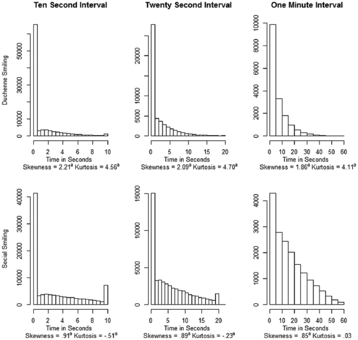
Histograms of smile duration.

As the data failed to meet distributional requirements for time-series analysis—a characteristic that will likely be common among data sets examining categorical codes—I did not apply traditional time-series methods to the current data set. Instead, I examined the relationship between Duchenne smiling across groupmates within a regression framework that shares many characteristics of time-series methods but offers more options in terms of the distribution of outcome variables (Fairbairn & Sayette, 2013; Kenny et al., 2006). More specifically, I estimated effects within hierarchical generalized linear models specifying Poisson distributed errors. Within this framework, I predicted an individual’s duration of Duchenne smiling during the current 10-s interval with that individual’s groupmates’ Duchenne smiling during the previous 10-s interval, controlling for the individual’s own Duchenne smiling during the previous 10-s interval. Results indicated that an individual’s agreeableness did not significantly moderate the relationship between groupmates smiling duration during the previous 10-s interval and that individual’s smiling duration during the current 10-s interval, B = −0.01, t = −1.64, p = .10. Thus, an individual’s level of agreeableness does not appear to significantly moderate the correlation between groupmates’ duration of Duchenne smiling during the previous 10-s interval and their current duration of Duchenne smiling. However, given characteristics of time-series analysis noted previously, it is unclear whether these results reflect (a) lack of concordance between an individual and his/her groupmates at the level of smiling or non-smiling, or (b) a time interval that is either too large or too small to capture concordance of smiling behavior.

The Nested Frailty Model

Next, the effect of agreeableness was examined using a nested frailty approach. This type of model is capable of integrating time as a continuous variable and is also well suited to the examination of categorical codes. More specifically, when applied to the current example, nested frailty models would address the question “what is the probability of an initial smile being reciprocated for each unit time that smile is displayed?” Thus, unlike popular event-level approaches, survival methods allow the researcher to model the exact duration of the initial smile, while avoiding the interpretive ambiguities that arise when time-series methods are applied to categorical behavioral observation codes.

For ease of comparison with previous event-level models, which have examined agreeableness only at the level of the group, I began by estimating a simple nested frailty model involving only one group-level predictor (Equation 4). Note that this first model does not necessarily require the nested frailty model, and might be estimated using basic frailty models.

L o g [h_{i j k} (t)] = \log [h_{0} (t)] + β_{001} {GA}_{k} + u_{k} + w_{j k}

Where GA represents the sum of group members’ level of agreeableness. Random effect w_jk represents the clustering of initial smiles (i) within individuals (j), and u_k the clustering of these smile initiators (j) within groups of three (k).

The data structure required for this nested frailty analysis is represented in Table 1. The data set should be in long form, with each row representing an occurrence of each behavior (antecedent condition in this case initial smiles are clustered within individuals (SubjectID), which are then clustered within groups (GroupID). The Mutual column, which functions as an indicator of whether or not an observation was censored, is a binary indicator of whether or not a smile led to a mutual smile (Mutual = 1) or ended without being reciprocated (Mutual = 0). Finally, the Duration column identifies the length of time a given behavior lasted before it either led to a mutual smile or ended without being reciprocated. In the results reported below, group differences in hazard rates are represented by the abbreviation Exp(B), which can be interpreted as a form of relative risk for transition across levels of a given predictor and provide information regarding the size of effects. Likelihood ratio tests comparing the relative fit of basic frailty models (only group random effect) versus nested frailty models (individual and group random effect) confirmed that the nested frailty model provided a significantly improved model fit, χ² = 157.29, p < .0001.

Table 1.

Example Data Structure for Nested Frailty Analysis.

GroupID	SubjectID	GrpAgree	ActAgree	PartAgree	Mutual	Duration
001	001	98	29	69	0	4.76
001	001	98	29	69	1	0.07
001	001	98	29	69	0	3.03
001	002	98	33	65	0	1.27
001	002	98	33	65	1	1.07
001	003	98	36	62	1	0.40
001	003	98	36	62	0	0.50
002	004	82	22	60	1	1.14
002	004	82	22	60	0	2.53
002	005	82	34	48	0	2.46
002	005	82	34	48	0	4.76
002	005	82	34	48	1	0.07
002	006	82	26	56	1	3.03
002	006	82	26	56	0	1.27

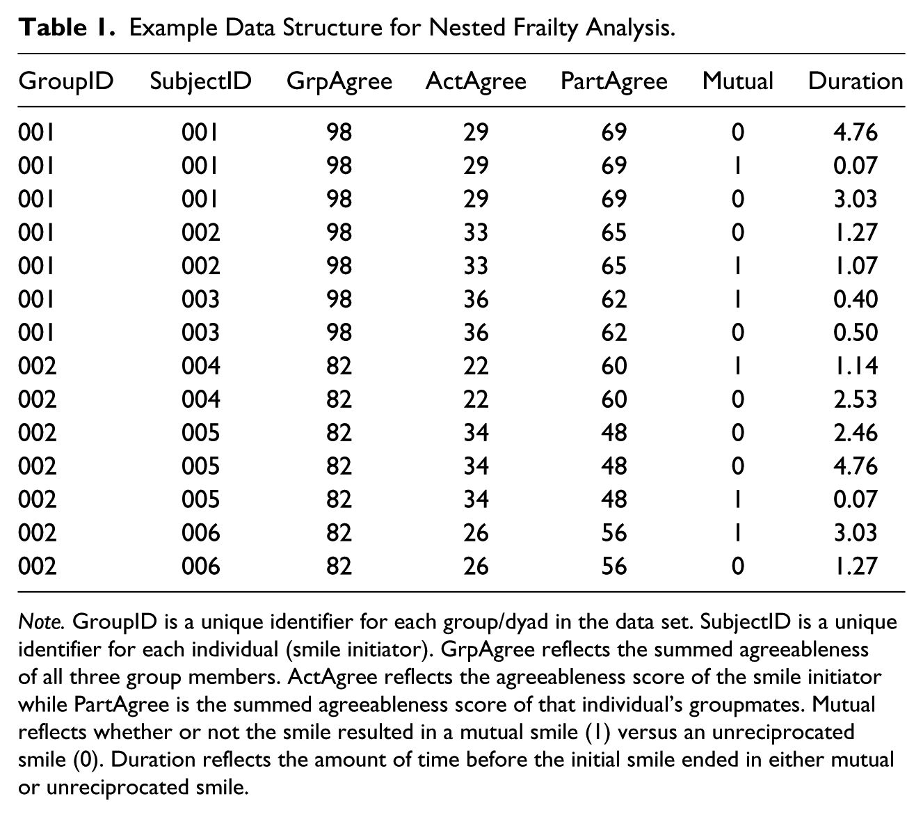
Note. GroupID is a unique identifier for each group/dyad in the data set. SubjectID is a unique identifier for each individual (smile initiator). GrpAgree reflects the summed agreeableness of all three group members. ActAgree reflects the agreeableness score of the smile initiator while PartAgree is the summed agreeableness score of that individual’s groupmates. Mutual reflects whether or not the smile resulted in a mutual smile (1) versus an unreciprocated smile (0). Duration reflects the amount of time before the initial smile ended in either mutual or unreciprocated smile.

In contrast to the previous event-level analysis, results of the nested frailty survival analysis of group agreeableness indicated no significant relationship between the group’s level of agreeableness and the probability that an initial smile would develop into a mutual smile within that group, B = 0.05, Exp(B) = 1.05, SE(B) = .03, p = .12. As noted previously, agreeableness was significantly associated with the duration of smiles, so that those higher in agreeableness showed longer initial smile duration. It was previously unclear whether event-level findings were attributable to true increases in social responsiveness within agreeable groups, or were instead simply attributable to longer initial smile duration within these groups. In light of null findings now produced within the survival framework, it seems that the association between group agreeableness and mutual smile transition was likely partially attributable to initial smile duration.

Importantly, however, to this point models have just examined predictors that vary at the level of the group. I have only examined the effect of a group’s level of agreeableness, and have not examined the characteristics of any individuals within the group. In other words, models have failed to parse the effect of being oneself highly agreeable with being in a group with highly agreeable people. Thus, to this point, the characteristics of the smile initiator are indistinguishable from the characteristics of the smile initiator’s groupmates. It is therefore unclear whether being oneself agreeable or, conversely, being in a group with highly agreeable people might increase the probability of a smile being reciprocated. Survival analytic models proposed to this point (Stoolmiller & Snyder, 2006) do not have the capability to examine predictors that denote characteristics of individuals, or factors that vary within indistinguishable dyads or small groups. Importantly, however, nested frailty models, which operate at three levels of analysis, can disentangle the contributions of an individual’s own characteristics from the characteristics of that individual’s groupmates.

Using the nested frailty approach together with Kenny and colleagues’ APIM, we can parse actor effects (characteristics of the smile initiator) from partner effects (characteristics of the smile initiator’s groupmates) and examine which of these factors might drive the effects reported to this point (Kenny, Mannetti, Pierro, Livi, & Kashy, 2002). This analytic strategy, as applied to the current research question, is represented in Equation 5.

L o g [h_{i j k} (t)] = \log [h_{0} (t)] + β_{010} {AA}_{j k} + β_{020} {PA}_{j k} + u_{k} + w_{j k}

Where AA represents the effects of actor (smile initiator) agreeableness and PA the effect of partner agreeableness (the summed agreeableness of the smile initiator’s two groupmates).

Results of these nested frailty models indicate that the agreeableness of the individual who initiates the smile (the actor) does not impact the hazard that a smile will transition into a mutual smile (see Figure 2). In other words, this study did not find evidence that smiles displayed by individuals high in agreeableness were more likely to develop into a mutual smile, per unit time they were displayed, p = .75. In contrast, models did produce evidence that the level of agreeableness of the smile initiator’s groupmates (partner effects, or effects of potential smile responders) influenced the probability that the initial smile would transition into a mutual smile, B = 0.07, Exp(B) = 1.07, SE(B) = .028, p = .02 Hazard to mutual smile increased by 7% for every one standard deviation increase in groupmates’ level of agreeableness.

Figure 2.

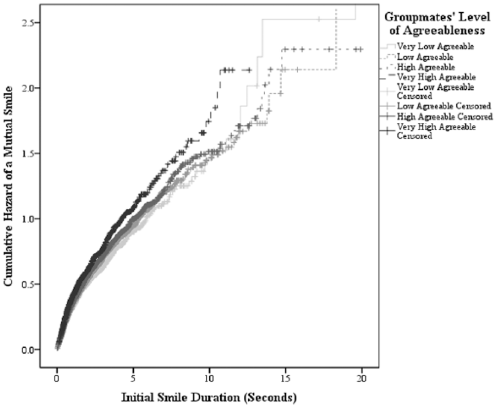
Cumulative hazard of a smile developing into a mutual smile as a function of groupmates’ agreeableness.

In sum, using the survival analytic framework, we found no evidence that a group’s average level of agreeableness increased the probability of a smile being reciprocated, per each unit time that smile was displayed. We were, however, able to use novel nested frailty survival methods, together with the Actor–Partner Interdependence Model, to move beyond the level of the group and differentiate the smile initiator’s level of agreeableness from the level of agreeableness of that individual’s groupmates. This model produced evidence that being in a group with individuals high in agreeableness significantly increased hazard to mutual smile. In other words, results suggested that smiles displayed by those high in agreeableness were no more likely to meet with a responding smile than smiles displayed by those low in agreeableness but, instead, that those high in agreeableness might be more likely to “catch” a smile. Thus, using nested frailty models together with the APIM, we gain critical information regarding the individuals acting within the group and the social processes potentially at play.

Extensions of survival methods

Survival methods offer several additional features that may address questions of interest to researchers. As these features are available within all survival methods, and are not specific to the nested frailty model proposed here, this article does not go into detail regarding these features, but aims to simply point to their existence and their potential application within the current example. First, within examinations of behavioral observation data, researchers are often interested in the question of whether effects of a given transitional probability are observed above and beyond what might be expected given base rates of consequent conditions. In other words, when applied to the research questions addressed here, we might be interested in whether those high in agreeableness are simply more likely to smile at any point, regardless of whether one of their groupmates is already smiling?⁴ If such questions are of interest, then survival methods allow the researcher to stratify models according to different antecedent conditions. For example, in the case of the current data set, we might examine the effect of agreeableness on smiling behavior at times when no group members are smiling versus at times when one other group member is already smiling (the difference between effects of agreeableness under these two conditions is non-significant in the current example, p > .05). See Appendix, as well as Stoolmiller and Snyder (2006) and Fairbairn, Sayette, Aalen, and Frigessi (2015) for further discussion of these procedures. Second, in certain cases, it may be of interest to know whether effects vary over the course of the duration of the antecedent condition. For example, are the effects of agreeableness on increased tendency to “catch” a smile seen immediately after the onset of an initiating smile, or do they emerge only after a delay? A description of these methods is offered within Allison (2012) and an application to behavioral observation data is provided within Fairbairn et al. (2015).

Discussion

This article builds on prior work by Stoolmiller and Snyder (2006) as well as Gardner and Griffin (1989; Griffin & Gardner, 1989) to propose a novel nested frailty model for the analysis of behavioral observation data. While advances in computer systems increasingly facilitate the recording of timed-event behavioral sequences, researchers still overwhelmingly favor analytic approaches that discard duration information. Thus, although survival approaches for behavioral observation data have been presented within psychology’s top journals, such methods have not yet gained popularity over event-based sequential approaches. This article aimed to inspire and facilitate the implementation of survival-based approaches through (a) proposing a novel nested frailty model that allows for more flexible implementation of survival methods beyond the distinguishable dyad and (b) explicitly comparing results produced by survival models with results produced by several popular methods through an example application, demonstrating the enhanced information that might be gained from survival models.

Findings of the present research indicate that the nested frailty survival approach has several advantages over three traditional methods. Results produced by event-level approaches failed to address whether effects of agreeableness were explained by the duration of the antecedent condition (initial smiles). In turn, the windowed event-level approach produced variable findings, and time-series analytic approaches led to ambiguities in interpretation when applied to our categorical data. In contrast, survival models provided unique information critical to the understanding of social processes. Survival models consider the duration of the social behaviors under examination and thereby allow for the exploration of whether effects are best explained by more prolonged exposure to the antecedent condition versus by true increases in social responsiveness. Further, and of particular importance, the nested frailty approach extended previous survival methods by allowing for the parsing of individuals acting within groups. Unlike previously proposed survival methods, the nested frailty approach permits an examination of whether effects of interest are driven by characteristics of the actor in the antecedent condition, or instead by the characteristics of that individual’s interaction partner(s).

The survival framework is a highly flexible modeling platform, and the research questions that can be accommodated within survival models are not limited to those examined here. The analyses in the current article focus on transitions to mutual smile versus unreciprocated smile. The probability of a smile transitioning into a mutual smile will not necessarily increase as a function of the duration of this initial smile, and therefore (although I argue that the duration of the antecedent condition will be of great relevance regardless of whether simultaneous behavior is a consequent condition of interest) the focus on simultaneous action in the present analysis is intended to provide an example in which the relevance of timing is readily apparent. Nonetheless, sequential examinations will not always involve transitions to simultaneous action or to binary outcome states. Of particular note, such examinations often involve transitions to numerous categorical consequent conditions. For example, within a work team, an idea proposed by one team member might be met with polite agreement, polite disagreement, or rude disagreement by another team member. In such cases, results can be stratified according to not only antecedent condition (as shown here) but also according to these different consequent conditions. Further, different random effects can be estimated for each of these distinct transitions, and hypotheses concerning the significance of these random effects can be tested (Stoolmiller & Snyder, 2006).

Relatedly, the survival analytic approach will not be appropriate to all research questions. This approach will be most suitable when one or both of the following conditions are met: (a) the probability of a consequent condition is likely to depend, at least in part, on the duration of the antecedent condition and/or (b) the timing of the consequent condition relative to the antecedent condition is of conceptual interest. When neither of these conditions are met, then survival analysis will likely not be appropriate. (e.g., If the researcher were interested in the probability of laughter following a joke, the transitional probability to laughter would not necessarily seem to increase systematically with the duration of the joke and, further, an examination of joke duration would not seem likely to produce information of great conceptual interest.) Note that I do not intend that survival analysis should always entirely replace event-level analyses as the preferred strategy, and this approach may in fact work nicely in conjunction with traditional event-level analytic approaches, with each approach supplying unique information.

Researchers may also be interested in examining the effects of session time on survival models (e.g., Are effects more pronounced at the beginning or end of the social interaction?) or in differential effects across multiple different sessions. Survival models can be stratified to these distinct sessions or according to different time intervals within a session, and results can be compared to examine whether effects evolve over time. Further, in the current research, identifying the specific characteristics of the group member associated with the consequent condition was not of critical importance. Instead, I am broadly interested in differentiating the characteristics of the antecedent actor from that individual’s groupmates, and so the APIM framework adopted here was appropriate. Indeed, within research examining dyadic group configurations, the APIM will identify the actor associated with the consequent condition. However, where research involves small groups and researchers are interested in targeting the specific characteristics of the consequent actor, survival models can be stratified according to the different consequent actors in the group, and then effects can be combined across strata.

Nested frailty methods might be useful in addressing a variety of questions of potential interest to small group researchers and, more broadly, to those interested in social interaction. For example, in groups of students working together on math problems, if an initial idea is proposed by a male, versus a female, might the group display a shorter latency to consensus regarding this idea? In conversations within work teams, do conversational silences last longer if the last person to speak within a group was a member of a minority racial group? During interactions among peer groups, following an episode of social exclusion, might individuals high in extraversion be quicker to recover and smile again? During interactions between same-sex couples, do levels of rejection sensitivity of oneself or one’s partner affect the speed with which a negative remark meets with a negative response?

Limitations and Future Directions

Some limitations and future directions are worth addressing. The most complicated model examined here involved approximately 31,000 data points and required 45 min to converge. All models were run on a laptop PC computer with a 64 bit operating system and 4 gigabytes of RAM. Where data sets are significantly larger (e.g., studies where numerous distinct categorical codes are of interest), processing time may become onerous and more powerful computers may be required. Further, in all survival models, the possibility of informative censoring should be explored.

Informative censoring refers to the situation in which observations that are censored represent an entirely different population of observations than those that are not censored. To use the current research questions as an example, informative censoring would suggest that the smile that ended unreciprocated represented a distinct form of smile, which (for example) would never have developed into a mutual smile regardless of how long it lasted. Sensitivity analyses such as those described by Allison (2012) should always be undertaken to examine how informative censoring might impact key findings (of note, results of these sensitivity analyses indicated that informative censoring was not cause for concern in the current example application). Next, serial dependence of observations over time may be a significant concern within some data sets. It should be noted that the specific models proposed in the current article do not account for autocorrelation of observations at adjacent points in time (see Chiu & Khoo, 2005). Finally, in some cases researchers may theorize that behavioral influence and behavioral timing operate along orthogonal dimensions, and such researchers may wish to estimate the degree of behavioral influence independent of the relative timing of effects. In other words, in some cases, researchers may postulate that the relative timing of behaviors does not necessarily reflect the degree of interpersonal influence during social exchange. The approach provided here is not intended to entirely supplant sequential approaches. Indeed, in some cases, an event-level examination of sequential ordering may represent an important first step. Instead, the survival approach outlined here is intended to provide a useful alternative when the relative timing of behaviors is thought to be relevant for the understanding of interpersonal influence during social exchange.

Summary and Conclusions

This article introduces a method intended to facilitate the examination of time within behavioral observation research. In their classic text Observing Interaction, Bakeman and Gottman (1997) refer to the tyranny of time and—based on the limitations of analytic procedures in use when their book was written—argue for the removal of time from observational data for the purposes of analysis. In the decades since this book was published, it is safe to say that time has been entirely stripped of any tyrannical influence it might once have held within the behavioral observation literature. Indeed, despite calls by methodologists for research that integrates duration information (Stoolmiller & Snyder, 2006; Warner, 1998), the large body of work examining sequential social behaviors has wholly neglected to consider the timing of responses. This article presents one method well suited to the examination of the precise duration of behaviors across a range of dyadic and group interactions.

Footnotes

Appendix

The following code can be used to fit a nested frailty model with the R package coxme. Here we focus on the effects of agreeableness. Variables that appear within this code correspond to those described in Table 1. The data set “OneSmile.csv” is provided within supplemental materials. The code below assumes that a data set is not already “attached.” Therefore, variables are identified with the name of the data set (e.g., “mydata”) followed by the $ symbol and the name of the variable (e.g., mydata$NumSmile). Note that R is case sensitive, so the correct case must always be specified in referring to variables and data sets.

##First install and then call coxme using the following code

install.packages(“coxme”)

library(coxme)

##import dataset, saved as csv files, and store it as an object with the name “mydata”

mydata <- read.table(“C:/users/Desktop/Files/OneSmile.csv”, header=TRUE,sep=“,”)

##Fit a basic Frailty Model

frailty.coxme <- coxme(Surv(mydata$Duration, mydata$Mutual) ~ mydata$ZGrpAgree +(1 | mydata$GroupID), data=mydata)

##show results

print(frailty.coxme)

##Fit a nested frailty model using APIM

Nest.frailty.coxme <- coxme(Surv(mydata$Duration, mydata$Mutual) ~ mydata$ZPartAgree + mydata$ZActAgree + (1 | mydata$GroupID/mydata$SubjectID), data=mydata)

##show results

print(Nest.frailty.coxme)

Acknowledgements

Thanks to Drs. Aidan Wright, Michael Sayette, Rebecca Warner, John Levine, and David Kenny for their helpful comments on earlier versions of this manuscript. Thanks also to Drs. Arnoldo Frigessi, Odd Aalen, Harald Weedon-Fekjær, and Terry Therneau for assistance with data analysis.

Declaration of Conflicting Interests

The author(s) declared no potential conflicts of interest with respect to the research, authorship, and/or publication of this article.

Funding

The author(s) disclosed receipt of the following financial support for the research, authorship, and/or publication of this article: This research was funded by National Science Foundation Graduate Research Opportunities Worldwide Grant (230165/F11) and National Science Foundation Graduate Research Fellowship (0753293-006) to Catharine Fairbairn and by National Institutes of Health Grant (R01 AA015773) to Michael Sayette. A portion of this article was drafted during the Fall of 2013 while the author visited the Department of Biostatistics at the University of Oslo. This research was also supported by National Institutes of Health Grant (R01 AA015773) to Michael Sayette.

Notes

Author Biography

Catharine E. Fairbairn is assistant professor of psychology at the University of Illinois at Urbana–Champaign, USA. Her work looks at social processes in small group interactions, and how alcohol’s affects these social processes.

References

Allison

P. D.

(2012). Survival analysis using SAS: A practical guide. Cary, NC: SAS Institute.

Atkins

D. C.

Gallop

R. J.

(2007). Rethinking how family researchers model infrequent outcomes: A tutorial on count regression and zero-inflated models. Journal of Family Psychology, 21, 726-735. doi:10.1037/0893-3200.21.4.726

Bakeman

(2004). Sequential analysis. In Lewis-Beck

Bryman

A. E.

Liao

T. F.

(Eds.), The SAGE encyclopedia of social science research methods (Vol. 3. pp. 1024-1026). Thousand Oaks, CA: Sage.

Bakeman

Gottman

J. M.

(1997). Observing interaction: An introduction to sequential analysis (2nd ed.). New York, NY: Cambridge University Press.

Bakeman

Quera

(1995). Log-linear approaches to lag-sequential analysis when consecutive codes may and cannot repeat. Psychological Bulletin, 118, 272-284. doi:10.1037/0033-2909.118.2.272

Bakeman

Quera

(2011). Sequential analysis and observational methods for the behavioral sciences. New York, NY: Cambridge University Press.

Boker

S. M.

Laurenceau

(2006). Dynamical systems modeling: An application to the regulation of intimacy and disclosure in marriage. In Walls

T. A.

Schafer

J. L.

(Eds.), Models for intensive longitudinal data (pp. 195-218). Oxford, UK: Oxford University Press.

Boker

S. M.

Rotondo

J. L.

King

(2002). Windowed cross-correlation and peak picking for the analysis of variability in the association between behavioral time series. Psychological Methods, 7, 338-355. doi:10.1037/1082-989X.7.3.338

Butler

E. A.

(2011). Temporal interpersonal emotion systems The “TIES” that form relationships. Personality and Social Psychology Review, 15, 367-393. doi:10.1177/1088868311411164

10.

Chan

(1998). Functional relations among constructs in the same content domain at different levels of analysis: A typology of composition models. Journal of Applied Psychology, 83, 234-246. doi:10.1037/0021-9010.83.2.234

11.

Chapple

E. D.

(1970). Culture and biological man. New York, NY: Holt, Rinehart and Winston.

12.

Chen

Chiu

M. M.

Wang

(2012). Social metacognition and the creation of correct, new ideas: A statistical discourse analysis of online mathematics discussions. Computers in Human Behavior, 28, 868-880. doi:10.1016/j.chb.2011.12.006

13.

Chiu

M. M.

Khoo

(2005). A new method for analyzing sequential processes dynamic multilevel analysis. Small Group Research, 36, 600-631. doi:10.1177/1046496405279309

14.

Costa

P. T.

McCrae

R. R.

(1992). Four ways five factors are basic. Personality and Individual Differences, 13, 653-665. doi:10.1016/0191-8869(92)90236-I

15.

Cox

D. R.

(1972). Regression models and life tables (with discussion). Journal of the Royal Statistical Society: Series B, 34, 187-220.

16.

Cronin

M. A.

Weingart

L. R.

Todorova

(2011). Dynamics in groups: Are we there yet? The Academy of Management Annals, 5, 571-612. doi:10.1080/19416520.2011.590297

17.

Dagne

G. A.

Brown

C. H.

Howe

G. W.

(2007). Hierarchical modeling of sequential behavioral data: Examining complex association patterns in mediation models. Psychological Methods, 12, 298-316. doi:10.1037/1082-989X.12.3.298

18.

Dagne

G. A.

Howe

G. W.

Brown

C. H.

Muthén

B. O.

(2002). Hierarchical modeling of sequential behavioral data: An empirical Bayesian approach. Psychological Methods, 7, 262-280. doi:10.1037/1082-989X.7.2.262

19.

Donders

F. C.

(1969). On the speed of mental processes. Acta Psychologica, 30, 412-431. doi:10.1016/0001-6918(69)90065-1

20.

Duchateau

Janssen

(2007). The frailty model. New York, NY: Springer.

21.

Ekman

Friesen

W. V.

Hager

J. C.

(2002). Facial action coding system. Salt Lake City, UT: Network Information Research.

22.

Ekman

Rosenberg

E. L.

(2005). What the face reveals: Basic and applied studies of spontaneous expression using the Facial Action Coding System (FACS) (2nd ed.). New York, NY: Oxford University Press.

23.

Fairbairn

C. E.

Sayette

M. A.

(2013). The effect of alcohol on emotional inertia: A test of alcohol myopia. Journal of Abnormal Psychology, 122, 770-781. doi:10.1037/a0032980

24.

Fairbairn

C. E.

Sayette

M. A.

Aalen

O. O.

Frigessi

(2015). Alcohol and emotional contagion: An examination of the spreading of smiles in male and female drinking groups. Clinical Psychological Science, 3, 686-701. doi:10.1177/2167702614548892

25.

Gardner

Griffin

W. A.

(1989). Methods for the analysis of parallel streams of continuously recorded social behaviors. Psychological Bulletin, 105, 446-455. doi:10.1037/0033-2909.105.3.446

26.

Gottman

J. M.

(1981). Time-series analysis: A comprehensive introduction for social scientists. Cambridge, UK: Cambridge University Press.

27.

Granic

Patterson

G. R.

(2006). Toward a comprehensive model of antisocial development: A dynamic systems approach. Psychological Review, 113, 101-131. doi:10.1037/0033-295X.113.1.101

28.

Graziano

W. G.

Jensen-Campbell

L. A.

Hair

E. C.

(1996). Perceiving interpersonal conflict and reacting to it: the case for agreeableness. Journal of Personality and Social Psychology, 70, 820-835.

29.

Graziano

W. G.

Tobin

R. M.

(2009). Agreeableness. In Leary

M. R.

Hoyle

R. H.

(Eds.), Handbook of individual differences in social behavior (pp. 46-61). New York, NY: Guilford Press. Retrieved from http://doi.apa.org/?uid=2009-12071-004

30.

Greenwald

A. G.

McGhee

D. E.

Schwartz

J. L.

(1998). Measuring individual differences in implicit cognition: The implicit association test. Journal of Personality and Social Psychology, 74, 1464-1480. doi:10.1037/0022-3514.74.6.1464

31.

Griffin

W. A.

Gardner

(1989). Analysis of behavioral durations in observational studies of social interaction. Psychological Bulletin, 106, 497-502. doi:10.1037/0033-2909.106.3.497

32.

Herndon

Lewis

(2015). Applying sequence methods to the study of team temporal dynamics. Organizational Psychology Review, 5, 318-332. doi:10.1177/2041386614538276

33.

Jadallah

Anderson

R. C.

Nguyen-Jahiel

Miller

B. W.

Kim

Kuo

. . . Wu

(2011). Influence of a teacher’s scaffolding moves during child-led small-group discussions. American Educational Research Journal, 48, 194-230. doi:10.3102/0002831210371498

34.

Jaffe

Beebe

Feldstein

Crown

C. L.

Jasnow

M. D.

Rochat

Stern

D. N.

(2001). Rhythms of dialogue in infancy: Coordinated timing in development. Monographs of the Society for Research in Child Development, 66, 1-132.

35.

Jaffe

Feldstein

(1970). Rhythms of dialogue. New York, NY: Academic.

36.

Kauffeld

Meyers

R. A.

(2009). Complaint and solution-oriented circles: Interaction patterns in work group discussions. European Journal of Work & Organizational Psychology, 18, 267-294. doi:10.1080/13594320701693209

37.

Kenny

D. A.

(1994). Interpersonal perception: A social relations analysis. New York, NY: Guilford Press.

38.

Kenny

D. A.

Kashy

D. A.

Cook

W. L.

(2006). Dyadic data analysis. New York, NY: Guilford Press.

39.

Kenny

D. A.

Mannetti

Pierro

Livi

Kashy

D. A.

(2002). The statistical analysis of data from small groups. Journal of Personality and Social Psychology, 83, 126-137. doi:10.1037/0022-3514.83.1.126

40.

Leenders

Contractor

N. S.

DeChurch

L. A.

(in press). Once upon a time: Understanding team dynamics as relational event networks. Organizational Psychology Review.

41.

Lehmann-Willenbrock

Allen

J. A.

(2014). How fun are your meetings? Investigating the relationship between humor patterns in team interactions and team performance. Journal of Applied Psychology, 99, 1278-1287. doi:10.1037/a0038083

42.

Lehmann-Willenbrock

Allen

J. A.

Kauffeld

(2013). A sequential analysis of procedural meeting communication: How teams facilitate their meetings. Journal of Applied Communication Research, 41, 365-388. doi:10.1080/00909882.2013.844847

43.

Liddle

H. A.

Dakof

G. A.

Parker

Diamond

G. S.

Barrett

Tejeda

(2001). Multidimensional family therapy for adolescent drug abuse: Results of a randomized clinical trial. The American Journal of Drug and Alcohol Abuse, 27, 651-688.

44.

Meier

B. P.

Robinson

M. D.

Carter

M. S.

Hinsz

V. B.

(2010). Are sociable people more beautiful? A zero-acquaintance analysis of agreeableness, extraversion, and attractiveness. Journal of Research in Personality, 44, 293-296.

45.

Ozechowski

T. J.

Turner

C. W.

Hops

(2007). Mixed-effects logistic regression for estimating transitional probabilities in sequentially coded observational data. Psychological Methods, 12, 317-335.

46.

Putnam

L. L.

(1983). Small group work climates: A lag-sequential analysis of group interaction. Small Group Research, 14, 465-494. doi:10.1177/104649648301400405

47.

Raudenbush

S. W.

Bryk

A. S.

(2002). Hierarchical linear models: Applications and data analysis methods (Vol. 2). Thousand Oaks, CA: Sage.

48.

Sadler

Ethier

Gunn

G. R.

Duong

Woody

(2009). Are we on the same wavelength? Interpersonal complementarity as shared cyclical patterns during interactions. Journal of Personality and Social Psychology, 97, 1005-1020. doi:10.1037/a0016232

49.

Sastry

(1997). A nested frailty model for survival data, with an application to the study of child survival in northeast Brazil. Journal of the American Statistical Association, 92, 426-435. doi:10.1080/01621459.1997.10473994

50.

Sayette

M. A.

Creswell

K. G.

Dimoff

J. D.

Fairbairn

C. E.

Cohn

J. F.

Heckman

B. W.

. . . Moreland

R. L.

(2012). Alcohol and group formation: A multimodal investigation of the effects of alcohol on emotion and social bonding. Psychological Science, 23, 869-878. doi:10.1177/0956797611435134

51.

Stachowski

A. A.

Kaplan

S. A.

Waller

M. J.

(2009). The benefits of flexible team interaction during crises. Journal of Applied Psychology, 94, 1536-1543. doi:10.1037/a0016903

52.

Sternberg

(1969). Memory-scanning: Mental processes revealed by reaction-time experiments. American Scientist, 57, 421-457.

53.

Stoolmiller

Snyder

(2006). Modeling heterogeneity in social interaction processes using multilevel survival analysis. Psychological Methods, 11, 164-177. doi:10.1037/1082-989X.11.2.164

54.

Therneau

(2011). Coxme: Mixed effects Cox Models (R Package Version).

55.

Warner

R. M.

(1998). Spectral analysis of time-series data. New York, NY: Guilford Press.

56.

Warner

R. M.

(2008). Applied statistics: From bivariate through multivariate techniques. Los Angeles, CA: Sage.

57.

Watzlawick

Bevelas

J. B.

Jackson

D. D.

(1967). Pragmatics of human communication. New York, NY: W.W. Norton.

58.

Wienke

(2010). Frailty models in survival analysis. Boca Raton, FL: CRC Press.

59.

Yoder

P. J.

Tapp

(2004). Empirical guidance for time-window sequential analysis of single cases. Journal of Behavioral Education, 13, 227-246. doi:10.1023/B:JOBE.0000044733.03220.a9