Life Span as the Measure of Performance and Learning in a Business Gaming Simulation

Abstract

This study applies the learning curve method of measuring learning to participants of a computer-assisted business gaming simulation that includes a multiple-life-cycle feature. The study involved 249 participants. It verified the workability of the feature and estimated the participants’ rate of learning at 17.4% for every doubling of experience. This method of measuring learning may be useful for the comparative assessment of different kinds of computer-mediated simulations and of their features and ancillary activities.

Keywords

assessment business simulation comparative assessment computer-assisted computer-mediated simulations experience learning curve learning measurement learning rate life cycle life span performance measurement

Consistent with the classical prescription of Campbell and Stanley (1963) on conducting psychological research, gaming simulation researchers have assessed learning using paper-and-pencil examinations by comparing the pretreatment and posttreatment responses of participants, or by comparing the response of a treatment group with that of a reference group, or by using both approaches (Gosen & Washbush, 2004). An exemplary instance of these efforts is the series of 11 studies undertaken over 8 years by Washbush and Gosen (2001), who applied two parallel forms of a paper-and-pencil examination for pretreatment and posttreatment comparisons. Although Washbush and Gosen showed that learning occurred from participation in simulations, despite their extensive efforts, they found little else, leading them to conclude, “There were few easily interpretable results . . . For the vast majority of predictor variables, relationships with learning were not significant” (p. 293). Their results corroborate earlier work by Anderson and Lawton (1992b), who found “very few significant relationships between the various measures of student learning and the student’s financial performance on the simulation exercise” (p. 337). Even with an updated literature review, Anderson and Lawton (2009) “have continued to be very disappointed with how little we can objectively demonstrate regarding what students learn from participating in simulation exercises” (p. 200).

The paucity of findings may be a consequence of the noise that accompanies the measurement of learning, because a paper-and-pencil examination of what simulation participants learn necessarily encompasses much that is not pertinent to performance in the simulation exercise itself, including test-taking skills, language skills, and cultural knowledge. For reasons such as these, learning is measured differently in operations management, by having the subject repeat the performance under controlled conditions, that is, conditions wherein noise is substantially limited. If the repetition gives rise to an improvement, learning has taken place, as evidenced by the improvement in performance that is observed. Thus, learning is defined behaviorally (Jonassen, 2003), based on what the subject does, rather than cognitively, based on a paper-and-pencil instrument that attempts to measure changes in the subject’s mental state.

In operations management, the amount of learning is calculated using a standard learning curve formula (Reguero, 1957; Wright, 1936), such that if T₁ is the time it takes to perform the task to an acceptable level of quality the first time and T_n is the time it takes to perform the same task to that same level of quality the nth time, then

T_{n} = T_{1} φ^{\log_{2} n} = T_{1} n^{\log_{2} φ} .

The measure of learning in Equation (1) is ϕ, the learning curve coefficient, which ranges between 0 and 1, inclusive. The general formula for computing ϕ is derived from Equation (1), so that given any mth and nth repetitions,

φ = 2^{\frac{\log (T_{n} / T_{m})}{\log (n / m)}} .

Accordingly, only two measurements of time are needed to estimate the learning curve coefficient, but if more than two are available, the data can be fitted by linear regression to the curve of Equation (1) to arrive at a best estimate. For this purpose, Equation (1) can be rearranged to reveal a linear relationship by taking its logarithm to any power; thus,

\log T_{n} = \log T_{1} + \log_{2} φ (\log n) .

Fitting Equation (3) to data is sensible only if the data come from times when the environment is sufficiently controlled to rule out events that distort measurement. These events are most likely to appear in the first few Ts, when the task is new, because the meaning of instructions may be unclear and extensive coaching may be provided. In the former case, the T that is observed would be contaminated by the time the subject took to understand the task; in the latter case, it would be contaminated by portions of the task that the instructor does for the subject to show how the work should be done. Accordingly, the data should not be fitted to Equation (3) until the Ts begin to fall, with repetition, along a curve.

The learning curve coefficient decreases when tasks are learned faster, so calling it a learning rate would be confusing. For clarity, the learning rate (ρ) can be defined as the complement of the learning curve coefficient, as follows:

ρ = 1 - φ

In descriptive terms, the learning rate is the relative reduction in the time to perform a task to an acceptable level of quality for every doubling of experience under controlled conditions. For example, if the learning curve coefficient is .95, then the time to perform the task falls by 5% with every doubling of experience. Thus, if a task takes an hour the first time, it should take 95% of an hour the second time (first doubling), (95%)² = 90.25% of an hour the fourth time (second doubling), (95%)³ = 85.74% of an hour the eighth time (third doubling), and so forth.

Learning rates in manufacturing operations differ depending on the combination of machine and manual labor that is employed. For assembly operations, which are largely manual, the learning rates are generally about 20% for every doubling of experience; for manufacturing operations, where the ratio of machine work to human work is about half and half, the learning rate is generally about 15%; and for operations where the ratio of machine work to human work is about three fourths to one fourth, the learning rate is generally about 10% (Andress, 1954).

The learning curve formula is based on the supposition that experience itself is sufficient for learning, a supposition supported by many studies on the educational effectiveness of business simulations (Gosen & Washbush, 2004; Washbush & Gosen, 2001; Wolfe, 1990, 1997), by the influential arguments of Dewey (1938, 1944), and by a large body of philosophical writing dating at least to the time of Socrates (Demiashkevich, 1935). The supposition is in tune with Dewey’s (1938) point that “every experience both takes up something from those which have gone before and modifies in some way the quality of those which come after” (p. 27). In other words, people are intelligent. When they perform a task repeatedly, they learn by themselves to work faster, provided they are neither inhibited from learning by disincentives nor prevented from working faster by machines—teaching is not necessary for learning.

Even so, Hirschmann (1964) cautions that performance improvements predicted by the learning curve formula do not arise merely because they are expected. He states, “It is not ordained by fate to arrive on schedule, but must be continuously, vigorously, and resourcefully sought” (p. 137). As such, if performance improvements by participants of a business gaming simulation are to appear as predicted by the formula, the participants must be substantially in control of their performance, be given incentives for improved performance, and be responsive to the incentives. The exposition that follows explains how a business gaming simulation that measures T was designed and administered to meet these conditions. Data are presented to show that T is a measure of performance that participants of the simulation accept, because their performance varied, as expected, with incentive conditions. A measure of the participants’ learning is then obtained by using linear regression to fit the data to Equation (3). The exposition concludes with suggestions for subsequent research.

The Gaming Simulation

The gaming simulation that was used to measure learning is GEO (2006), a computer-assisted simulation of a global economy. As a computer-assisted simulation the simulation couples high participant-participant interaction with high participant control (Crookall, Martin, Saunders, & Coote, 1986). Consistent with the importance accorded to participant-participant interactions, the GEO simulation program tracks each participant, requiring each to log into the simulation program with a unique user name and password. Consistent with high participant control, companies are not thrust on participants to manage. Rather, participants are allowed to found companies whenever they choose, distributing the shares of the founded companies among themselves in whatever proportion they find fitting. Thus, some companies might have one shareholder, whereas others have five; some participants might own shares in only one company, whereas others might own shares in five companies. Participants are neither restricted to working for the company in which they own shares nor prevented from moonlighting, that is, working in more than one job, so a participant might be employed as a manager of one company, a purchasing agent of another, and a sales agent of a third. Participants are prevented from doing the same job for more than one company, as that would be a conflict of interest. Essentially, GEO enables participants to do much of what people do in everyday commerce, namely, choose their associates and the nature of each association. It differs from everyday commerce in that antisocial actions, such as theft and embezzlement, are largely forestalled by the computer, rather than discouraged by the threat of law enforcement.

Distinguishing Features

GEO goes beyond the total enterprise (Goosen, Jensen, & Wells, 2001; Keys, 1987, 1997) to encompass a global economy. Its distinguishing features include how it handles time, sales, teams, and the objective of play.

Unlike many business simulations used in educational settings (Biggs, 1990; Fritzsche & Cotter, 1990), wherein time is administratively driven, and the entire duration of the exercise is completed in no more than 16 periods (Anderson & Lawton, 1992a; Rollier, 1992), GEO’s time is clock and activity driven (Chiesl, 1990; Thavikulwat, 1996) and set to advance automatically at the pace of about 50 periods a week after the initial registration and startup phases. Like the other business simulations, when a period advances goods are produced, income is paid, interest is charged, and taxes are collected.

In GEO, sales of products and stocks are not determined by a mathematical model of the market. Instead, sales are the result of auctions supported by the simulation program, so the participants’ principal challenge lies not in finding the solution to a model of the market but in sensing the ebb and flow between cooperation and competition that enables real markets to be adaptive and efficient (Thavikulwat, 1997).

In GEO, no one is required to join a team. Teams do form, nonetheless, because of an endogenous incentive: The production level of each company increases with the number of different participants employed by the company. Considering that the members of these teams have well-defined roles, as shareholders, managers, purchasing agents, and sales agents, and that any member can change teams at any time, the teams of GEO are more akin to those of the everyday world than to student teams put together for many other business simulations, wherein roles are often poorly defined (Teach, 1993; Wolfe & Rogé, 1997), and participants are not allowed to move from one team to another at will.

In GEO, consumption, rather than profit, is the objective of play (Thavikulwat, 1990, 2004). Each participant is assigned to be a citizen of a nation, and each is given a periodic cash entitlement. Participants expend their entitlements by founding companies, investing in the shares of companies, and purchasing company products for their own virtual consumption. Participants score higher by consuming more and consuming more evenly over the course of the exercise. Their consumption depends on their income, and their income includes salaries, dividends, and capital gains that in turn depend on their employment and ownership of company shares. As a consequence, participant scores are based on individual performance and only indirectly dependent on team or company performance.

Processes

The process through which participants receive their scores is diagrammed in Figure 1. The process begins with participation and ends with score. Although different scoring formulas apply to different administrative settings, all scoring formulas are based on consumption, measured in consumption points, and accumulated as participants purchase the virtual products produced by their virtual companies through a periodic double auction process that is procedurally simple but strategically complex (Thavikulwat & Pillutla, 2008).

Figure 1.

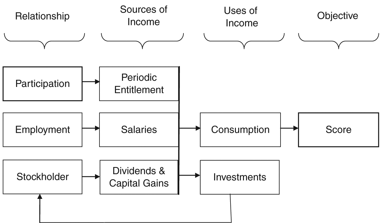
Performance flow diagram

Companies in GEO produce five kinds of products: service, material, energy, chemical, and food. Each kind of product is produced by companies specializing only in that product. The consumption points of each service and food item is the same to all participants, but the consumption points of each material, energy, and chemical item differ depending on the nation of which the participant is assigned to be a citizen. The supply chain of products and their consumption points per item is shown in Figure 2.

Figure 2.

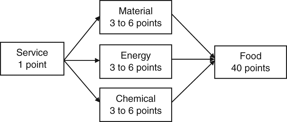
Supply chain of products and consumption points

The driving logic of the system is that no participant can earn a score without purchasing products for his or her own virtual consumption, no product can be produced without some participants founding companies to produce the products, no company can be founded without a participant choosing to invest some part of his or her periodic cash entitlements in founding a company and purchasing its shares, and no company can sell any of its production without a participant to purchase products, either for the participant’s own consumption or as a resource for the downstream company in which the participant is employed as a purchasing agent. The computer assists the participants in all these steps, but leaves the decision to act entirely with each participant.

The Study

The study reported here draws on data gathered when a multiple-life-cycle feature was added to the simulation. Before the addition, the simulation included only a single life cycle that began when the exercise started and ended when the exercise concluded. The problem with the single life cycle is that learning how to operate the simulation tends to take up a substantial part of the exercise (Wolfe & Castroviovanni, 2006), so the reliability of performance as a measure of participants’ capabilities is compromised. The multiple–life cycle feature isolates learning how to operate the simulation to the first life cycle, which should improve the reliability of performance as a measure of participants’ capabilities in subsequent life cycles. As implemented, companies remain intact throughout the exercise, but participants moving from one life cycle to the next lose all of their possessions, including their jobs and their company shares, so they begin each new life cycle from scratch.

In the process of refining the multiple–life cycle feature, the simulation was administered three different ways: by fixing the target, fixing the life span, and marking the segment. Each method requires its own measure of performance.

Fixing the target means that the administrator sets a fixed number of consumption points that participants must reach to complete a life cycle. This method is illustrated in Figure 3A, where the performance of Subject 1 (solid line) exceeds the performance of Subject 2 (dashed line), because Subject 1 reaches the target in fewer periods. With this method, each participant’s performance is measure by that participant’s life span, the number of periods that participant took to complete a life cycle.

Figure 3.

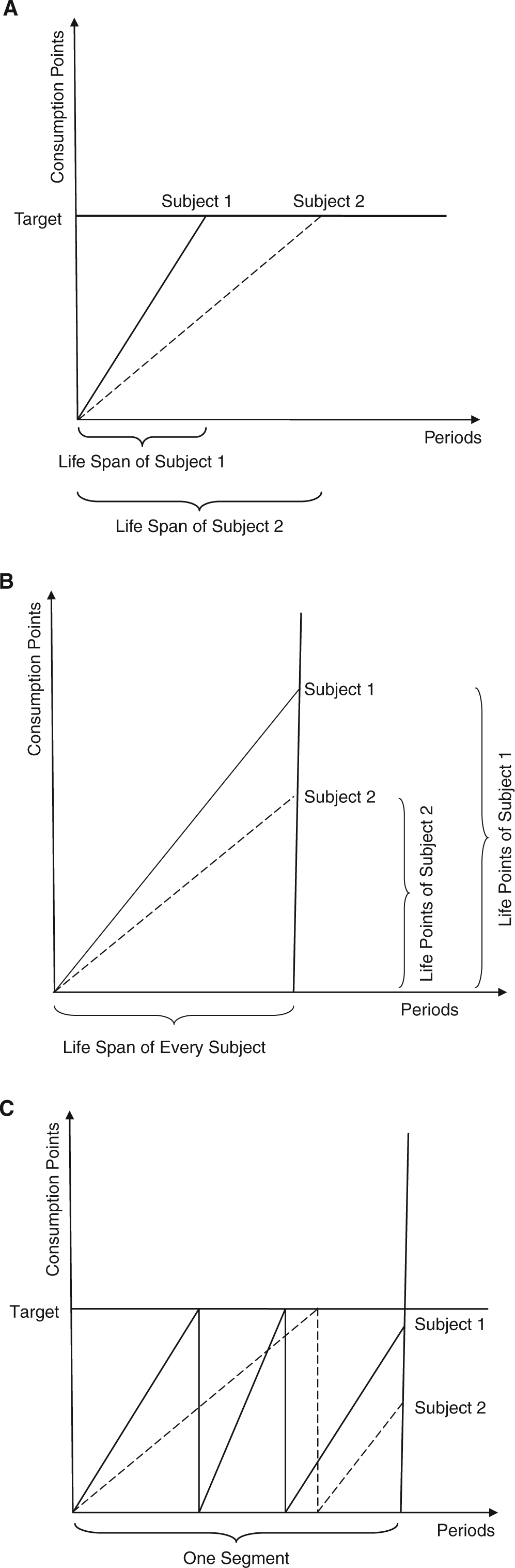
Three methods of administration: (A) fixing the target, (B) fixing the life span, and (C) marking the segment

Fixing the life span means that that the administrator sets the length of a life cycle to a fixed number of periods. This method is illustrated in Figure 3B, where the performance of Subject 1 (solid line) exceeds the performance of Subject 2 (dashed line), because Subject 1 receives more consumption points over the life cycle of identical length for both. With this method, each participant’s performance is measured by that participant’s life points, the number of consumption points received for consuming products within a life span of fixed length.

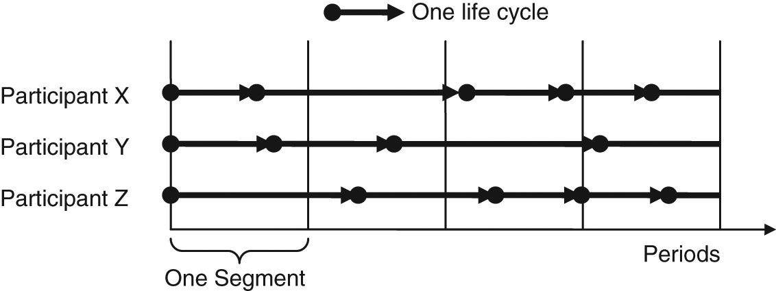
Marking the segment means that the administrator sets a target for completing each life cycle, allows participants to proceed automatically and immediately from one life cycle to the next until the exercise ends, and marks a segment as having been completed when a fixed number of periods have elapsed. This method is illustrated in Figure 3C, where the performance of Subject 1 (solid line) of almost three life cycles completed exceeds the performance of Subject 2 (dashed line) of about one and a half life cycles completed, over a segment of identical length for both. With this method, each participant’s performance within each segment is measured by the number of life cycles completed within that segment of the exercise.

Hypotheses

The simulation was administered under two incentive conditions: early performance annulled (EPA) and early performance incentivized (EPI). The incentive conditions are not treatments designed for the study but variations in conduct that were motivated by administrative and pedagogical concerns incidental to the study. It is fortuitous that these conditions serve the purpose of the study, inasmuch as the study was conceived after the data became available.

In the EPA condition, the simulation was administered by fixing the target for only the first two life cycles, with each participant proceeding automatically to the second life cycle on completing the first one. The exercise paused at two completed life cycles. Those who complete their first two life cycles earlier (early finishers) waited for those who took more time (late finishers), with everyone receiving the same credits toward grades, irrespective of their performance over their first two life cycles. Thus, performance over the first two life cycles was annulled, because performance had no effect on grades. The EPA condition is illustrated in Figure 4, where Participant X, on finishing the first two life cycles, waits for Participants Y and Z. The third and fourth life cycles were administered by fixing the life span, so all participants began and ended their life cycles simultaneously. Performance over the third and fourth life cycles affected grades.

Figure 4.

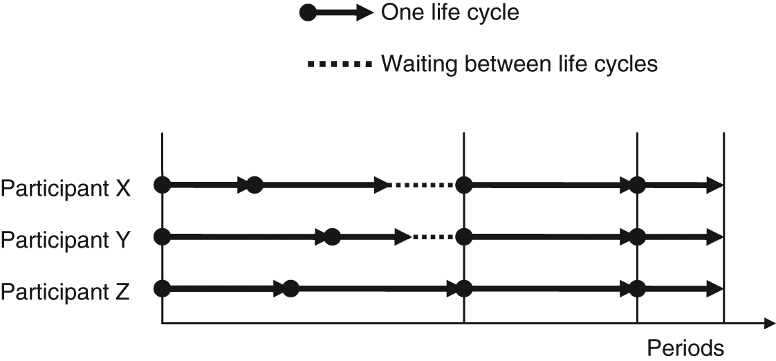
Participant X waits for Participants Y and Z after completing the first two life cycles, EPA condition

In the EPI condition, the simulation was administered by marking the segment, so each participant proceeded automatically from one life cycle to the next until the administrator ended the exercise. The EPI condition is illustrated in Figure 5. Performance over every life cycle affected grades.

Figure 5.

Each participant proceeds immediately to the next life cycle on completing the previous one, EPI condition

The rationale for EPA is that it promotes learning early in the exercise, because those who expend more time and effort to learn in the first life cycle, by methods such as taking more time to make decisions and intentionally making apparently poor decisions to gage consequences, are assured of suffering no loss in credits toward grades. Their early learning should improve performance in subsequent stages of the exercise. If this rationale is correct, then participants who spend more time in their first life cycle should perform better in their second life cycle than those who spend less time, because with more time-on-task in the first life cycle, they should have learned more then and applied their learning to their second life cycle. The first life span should therefore correlate negatively with the second life span, so the first hypothesis of the study is as follows:

Hypothesis 1: When early performance is annulled, life spans of the first life cycle will correlate negatively with those of the second life cycle.

The rationale for EPI is that it uses participants’ time more efficiently than EPA, because early finishers do not wait for late finishers, but this also means that those who take more time to learn early in the exercise pay a price in lower credits toward grades, which may not be completely recovered by better performance later. Considering therefore that participants must balance between learning and performance in the early periods of the simulation experience, the number of life cycles completed in the first segment (see Figure 5) of the exercise should not correlate with those of later segments, but the number of life cycles completed in later segments should be reliable, that is, they should correlate positively with each other. Accordingly, the second hypothesis of this study is as follows:

Hypothesis 2: When early performance is incentivized, the number of life cycles completed in the first segment will not correlate with the number of life cycles completed in later segments, whereas the number of life cycles completed in the second, third, and fourth segments will correlate positively with each other.

When extensive coaching is limited to the first life cycle of the simulation exercise, participants who complete more than two life cycles under EPI should demonstrate performance improvements attributable to learning, as evidenced by shorter life spans in subsequent life cycles. Even so, linking grades to early performance may induce an optimal level of arousal for some and a supra-optimal level for others. As Ariely, Gneezy, Loewenstein, and Mazar (2009) have shown, the supra-optimal arousal effect of high incentives can have detrimental consequences on performance in games, an effect commonly described as “choking under pressure” (Baumeister, 1984). On the expectation that the pressure of the EPI condition does not reach the point of inducing a supra-optimal level of arousal on the majority of the participants, the third hypothesis is as follows:

Hypothesis 3: When early performance is incentivized, the majority of participants who complete more than two life cycles will experience shorter life spans in subsequent life cycles.

The last hypothesis, applying also to the EPI condition, is the overall test of the arguments that life span is a reasonable measure of performance and learning, that learning occurs with experience even in the absence of teaching, that repetition gives rise to measurable learning, and that the learning rate falls along a logarithmic curve that fits the learning curve formula. The hypothesis is as follows:

Hypothesis 4: When early performance is incentivized, the mean performance of participants who complete more than two life cycles will fit the learning curve formula with a learning rate exceeding zero.

Method

The simulation exercise was a component of an undergraduate international business course involving 65 students in the first semester, 87 in the second, and 97 in the third. Three sections of the class were involved in each semester, with the students of each section constituting the citizens of one of three nations. Classes met twice a week in a computerized classroom, where each participant had access to a personal computer. Participants were encouraged to work on the simulation before and at the beginning of every class period, with entire class periods allotted at the beginning of the semester and tapering off to about 5 minutes per class period toward the end of the semester. Participants also could access the simulation from other computers on the campus at any time. In the second and third semesters, access from off campus through the Internet was enabled by an Internet-based (Pillutla, 2003) version of the simulation program. The exercise took place over the entire semester for all three semesters. The number of periods that elapsed in the three semesters was 787, 692, and 482, respectively. In every semester, the instructor coached the participants extensively during the first life cycle and limited assistance afterward only to those who requested it.

EPA Condition

Students of the first semester were involved in the EPA condition. They were told that the exercise would encompass four sequential life cycles. They would each earn 10 course points out of a grand total of 200 course points for each of the first two life cycles and a variable number of course points not exceeding 15 depending on their performance in completing each of their remaining two life cycles. Those who completed their first two life cycles earlier would simply get their work done sooner. They would earn no more in course points than those who either took more time or failed to complete their life cycles in the time allotted. Accordingly, the emphasis of the first two life cycles was more on learning relative to performance, because performance did not affect course points. In contrast, the emphasis of the last two life cycles was more on performance relative to learning, because performance translated into a difference in course points.

Even so, the students were told that performance in each of the last two life cycles counted toward grades only if it would raise their grades. Course percentage scores on which grades were based were calculated as follows: The number of course points allotted for the exercise was 10 + 10 + 15 + 15 = 50, leaving 150 points for the rest of the course. A student who earned 99 course points in the rest of the course would receive an initial course score of 66% (99 of 150). Adding the 20 course points assured to every student who participated in the first two life cycles of the exercise, the student’s revised course score would be 70% (119 of 170). If the student earned 10 and 14 course points for the last two life cycles, respectively, the student’s final course score would be 71.5% (119 + 10 + 14 out of 200). On the other hand, if the course points of the last two life cycles were reversed, so as to be 14 and 10, respectively, the student’s final course score would be 71.9% (119 + 14 out of 185). In this last case, the student’s performance in the last life cycle would be dropped because it would otherwise lower the course score to 71.5%, therefore negatively affect the student’s grade.

To complete each of the first two life cycles, participants had to consume products sufficient to reach two subtargets, one for absolute consumption and the other for relative consumption. The first subtarget was the sum of the absolute consumption points associated with each product that participants bought from producing companies through the simulation’s auction market. The second subtarget was the sum of the relative consumption scores that participants earned in each period. The relative consumption scores depended in an exponentially declining fashion on how much each participant consumed relative to the average consumption level of all participants, such that increasing consumption gave rise to increasing contributions to the relative consumption score, but at a decreasing rate. As a result, those who consumed more and consumed more evenly reached the target sooner, and so had shorter life spans than others.

Participants were allowed 8 weeks to complete the first two life cycles. At the end of the 8 weeks, the positions of those who had failed to complete two life cycles were set to two life cycles completed, and all participants were given 20 course points for their participation, as promised.

As for the last two life cycles, the life span was fixed, so targets did not apply. The third life cycle was administered for 4 weeks: the fourth, for 2 weeks. At the conclusion of each of these last two life cycles, performance was assessed by an exponential formula that gave 0% of the allotted course points to the participant who consumed nothing, 90% to the participant who consumed at the average level, and 100% to the participant who consumed at three times the average level or more.

EPI Condition

Students of the second and third semesters were involved in the EPI condition. As with the EPA condition, participants had to consume products to reach the target of each life cycle. Different from that condition, they were told that they could each complete up to five life cycles and that 10 course points would be added to their earned points and also to their basic totals, beginning at 150 basic points, for every life cycle completed. So, a student who completed two and a half life cycles would have 25 additional earned points and be graded with reference to a basis of 150 + 25 = 175 points, whereas a student who completed four life cycles would have 40 additional earned points and be graded with reference to a basis of 150 + 40 = 190 points. Fractional life cycles were calculated to equal the proportion of target that the student had reached when the exercise was terminated. The students were informed that the intent of the scoring system was to make performance in the gaming simulation a no-loser experience, that is, their grades could only be affected positively by their performance.

As with the first two life cycles of the EPA condition, those who consumed more and consumed more evenly reached the target sooner, so they had shorter life spans. Whereas in the EPA condition the early finishers of each of the first two life cycles waited for the later finishers, in the EPI condition each advanced immediately to the next life cycle on completing an earlier one.

Results

Descriptive statistics of life spans and life points under the EPA condition are presented in Table 1. Life Span 1 and Life Span 2 refer to the life spans of the first and second life cycles, respectively; Life Point 3 and Life Point 4 refer to the life points of the third and fourth life cycles, respectively. In the 8 weeks allotted for the first two life cycles, about 98% of the participants completed at least one life cycle, and about 57% completed at least two. As for the last two life cycles, every participant earned life points in the third, but about 15% earned none in the fourth.

Table 1.

Descriptive Statistics of Life Span and Life Points, EPA Condition

	Life Cycle
Item	1	2	3	4
No. of participants completing the life cycle	64	37	65	65
Measurement	Life Span 1	Life Span 2	Life Point 3	Life Point 4
Unit of measurement	Periods	Periods	Points	Points
Mean	208.95	185.27	6116.49	3251.28
SD	92.75	48.29	4737.44	4132.87

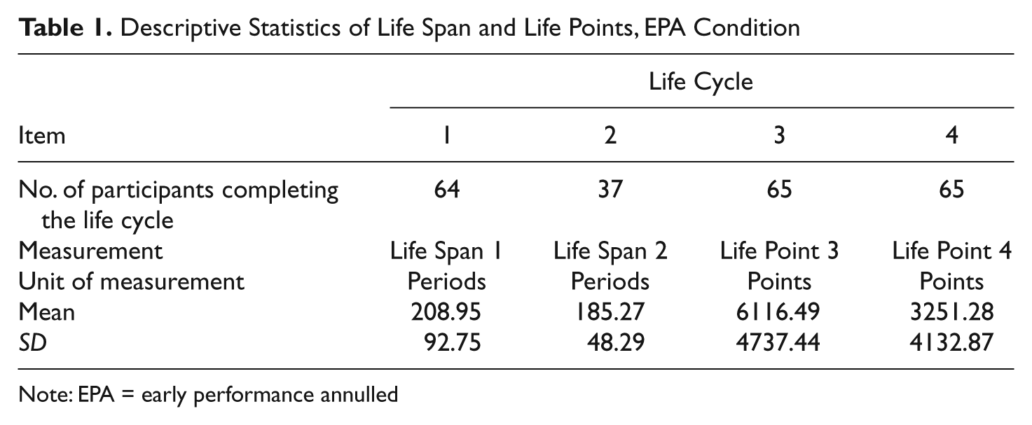
Note: EPA = early performance annulled

Pearson correlations of life spans and life points under the EPA condition are presented in Table 2. The positive correlation between Life Point 3 and Life Point 4 attests to the reliability of the life points measure. The negative correlation between Life Span 1 and Life Span 2 supports Hypothesis 1: When early performance is annulled, life spans of the first life cycle will correlate negatively with those of the second life cycle.

Table 2.

Pearson Correlation of Life Span and Life Points, EPA Condition

	Life Span 2	Life Point 3	Life Point 4
Life Span 1	−.580* (p = .000)	−.067 (p = .597)	−.023 (p = .856)
Life Span 2		−.175 (p = .299)	−.159 (p = .348)
Life Point 3			.586* (p = .000)

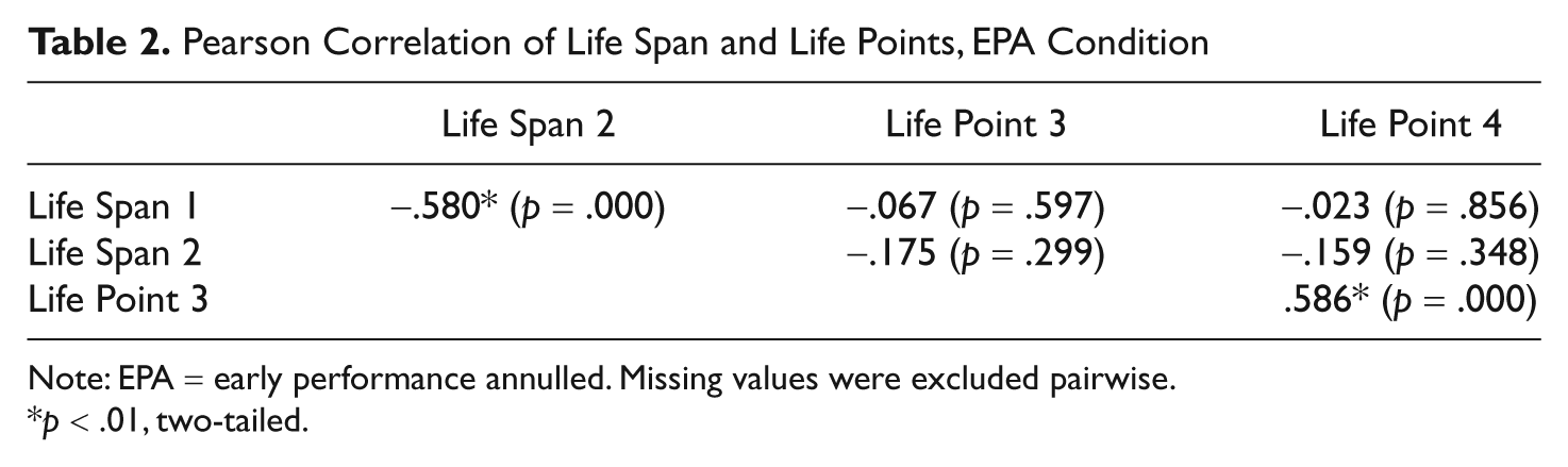
Note: EPA = early performance annulled. Missing values were excluded pairwise.

p < .01, two-tailed.

Descriptive statistics of life cycles completed under the EPI condition are presented in Table 3. The data are broken down by segments, with each segment consisting of one fourth of the total number of periods elapsed. Partial correlations of life cycles completed under the EPI condition, after controlling for semester, are presented in Table 4. As shown, Segment 1 is uncorrelated with performance in the other segments, whereas Segment 2, Segment 3, and Segment 4 are positively correlated with each other, supporting Hypothesis 2: When early performance is incentivized, the number of life cycles completed in the first segment will not correlate with the number of life cycles completed in later segments, whereas the number of life cycles completed in the second, third, and fourth segments will correlate positively with each other.

Table 3.

Descriptive Statistics of Life Cycles Completed, EPI Condition

Semester	Segment 1	Segment 2	Segment 3	Segment 4
First
Elapsed periods	1-173	174-346	347-519	520-692
No. of participants	87	87	87	87
Mean life cycles completed	1.049	0.875	0.773	0.690
SD	0.225	0.372	0.571	0.504
Second
Elapsed periods	1-121	122-241	242-362	363-482
No. of participants	97	97	97	97
Mean life cycles completed	0.793	0.468	0.653	0.587
SD	0.328	0.441	0.437	0.409

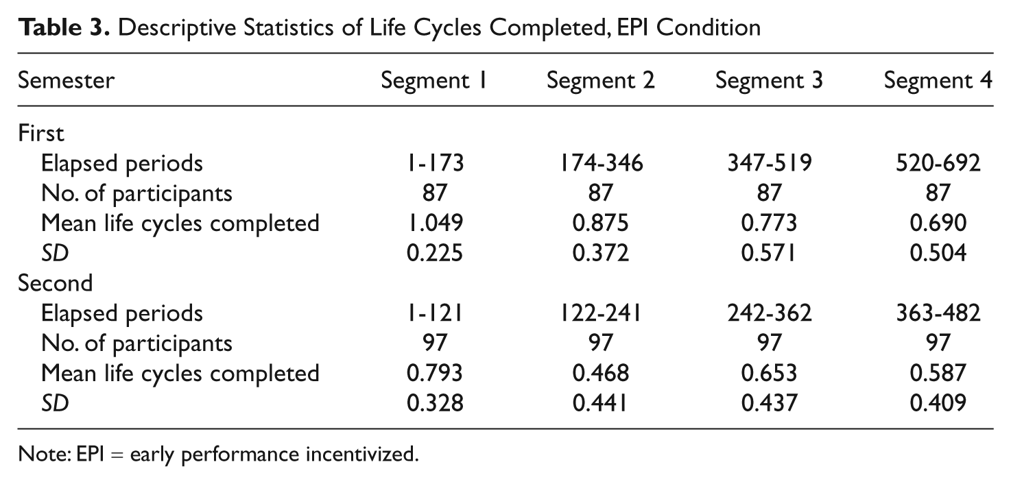
Note: EPI = early performance incentivized.

Table 4.

Partial Correlation of Life Cycles Completed, EPI Condition

	Segment 2	Segment 3	Segment 4
Segment 1	.005 (p = .948)	.065 (p = .385)	.072 (p = .331)
Segment 2		.357* (p = .000)	.277* (p = .000)
Segment 3			.390* (p = .000)

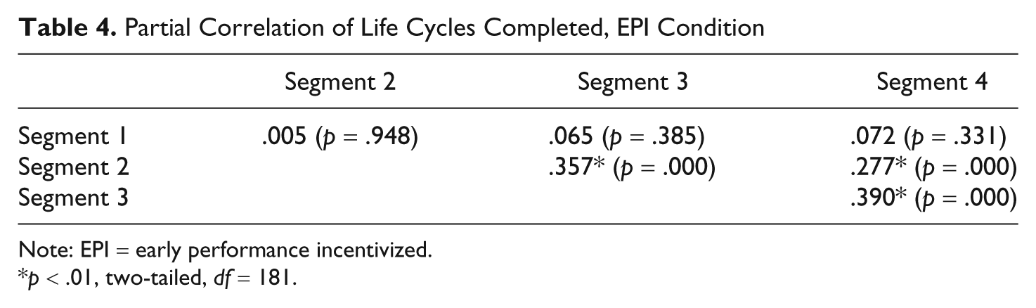
Note: EPI = early performance incentivized.

p < .01, two-tailed, df = 181.

Figure 6 presents the average performance patterns of participants in the EPI condition over the entire semester, broken down by last life cycle completed (LLC), beginning with LLC0 (completed one life cycle only) and ending with LLC4 (completed five life cycles). Every participant completed at least one life cycle in the second semester, but four, whose performances therefore do not appear on the graph (Figure 6B), did not complete even one in the third semester.

Figure 6.

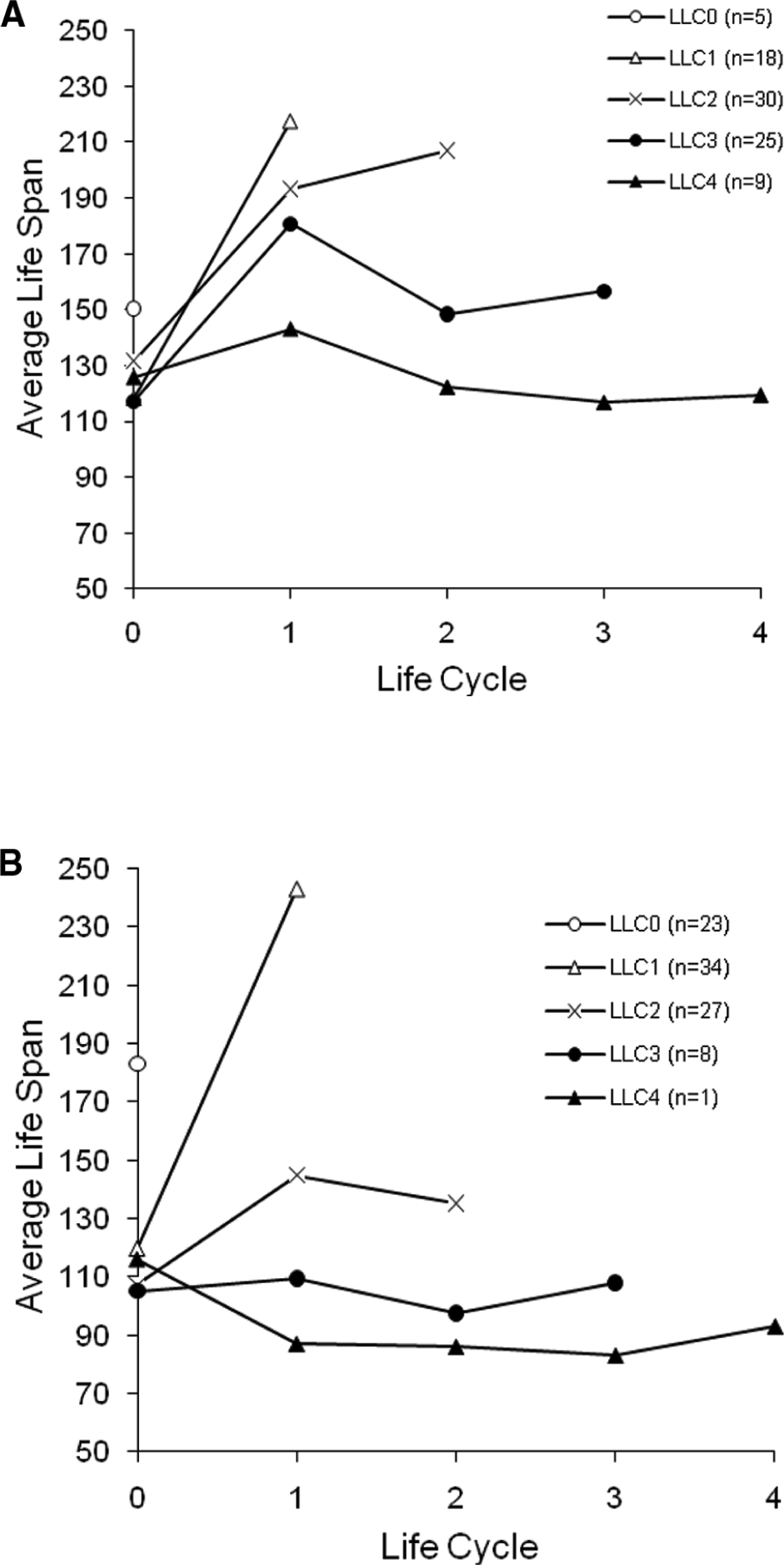
Average performance patterns of the (A) second and (B) third semesters by last life cycle completed, EPI condition

Figure 6 shows that, in both semesters, the range of average life spans at Life Cycle 0 is much narrower than the range of average life spans at Life Cycle 1. The difference is attributable to the extensive coaching given to everyone at the start of the exercise, so participants’ performance in Life Cycle 0 is a poor reflection of their abilities. Participants received limited assistance in Life Cycle 1 and beyond, so their performance in those life cycles is a better reflection of their abilities. Thus, the first T for the learning curve formula is the life span of Life Cycle 1.

Table 5 shows the proportion of participants in the EPI condition whose performance improved, as indicated by a reduced life span, from one life cycle to the next. Only 17.1% of those who completed the first two life cycles improved their performance from the first life cycle (LC0) to the second (LC1), whereas 58.0% to 60.0% of participants who completed more than two life cycles improved in subsequent life cycles, supporting Hypothesis 3: When early performance is incentivized, the majority of participants who complete more than two life cycles will experience shorter life spans in subsequent life cycles.

Table 5.

Proportion Whose Life Span Decreased Between Life Cycles, EPI Condition

Life Cycles	No. of Participants	Proportion Whose Life Span Decreased
From LC0 to LC1	152	17.1%
From LC1 to LC2	100	58.0%
From LC2 to LC3	43	58.1%
From LC3 to LC4	10	60.0%

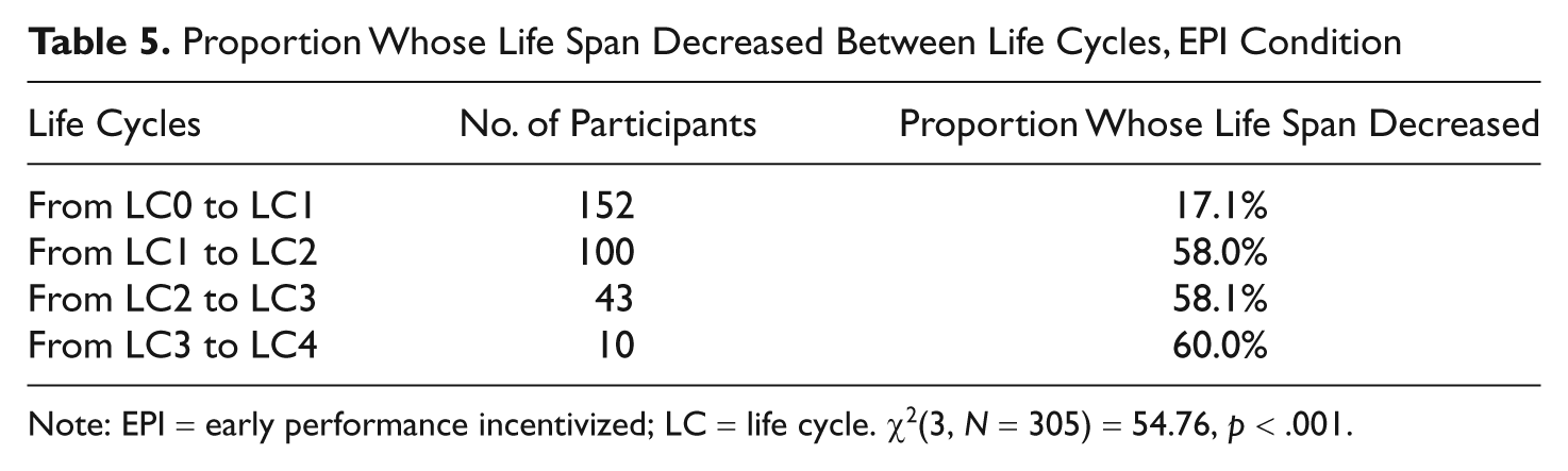
Note: EPI = early performance incentivized; LC = life cycle. χ²(3, N = 305) = 54.76, p < .001.

Table 6 presents description statistics for the two semesters of the EPI condition, and Table 7 presents the results of regressing, in accord with the linear relationship of Equation (3), the eight observations of the natural logarithm of the life cycles (log n) to the natural logarithm of the mean life spans (log T_n), with a dummy variable accounting for the two different semesters. The regression estimate of ϕ is 2^−0.276 = .826, so the estimated learning rate (Equation 4) is 17.4% for every doubling of experience. The 95% confidence interval of the learning rate is between 24.5% and 9.6% for every doubling of experience. These results support Hypothesis 4: When early performance is incentivized, the mean performance of participants who complete more than two life cycles will fit the learning curve formula with a learning rate exceeding zero.

Table 6.

Life Span of Each Life Cycle, EPI Condition

	Life Cycle
	1	2	3	4
Second semester
No. of participants	64	64	34	9
Mean life span	181.23	172.17	146.03	119.33
SD of life span	49.51	62.61	45.36	18.43
Third semester
No. of participants	36	36	9	1
Mean life span	135.31	125.53	105.22	93
SD of life span	44.04	36.20	23.00

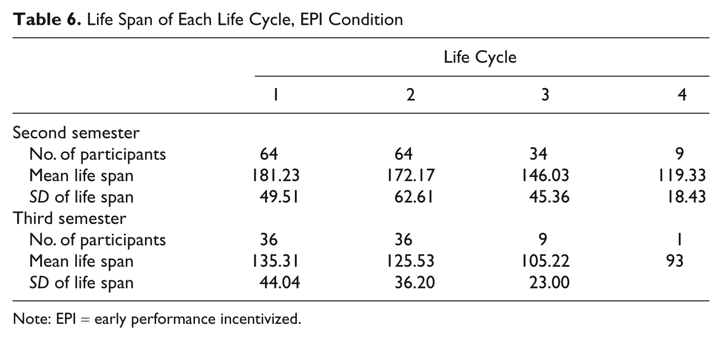
Note: EPI = early performance incentivized.

Table 7.

Logarithmic Regression of Life Cycle on Life Span, EPI Condition

	Coefficient	t	p
Intercept (log T₁)	5.248	95.70	.000
Slope (log₂ ϕ)	−0.276	−5.45	.003
Dummy (Semester 2, 0; Semester 3, 1)	−0.296	−5.62	.002

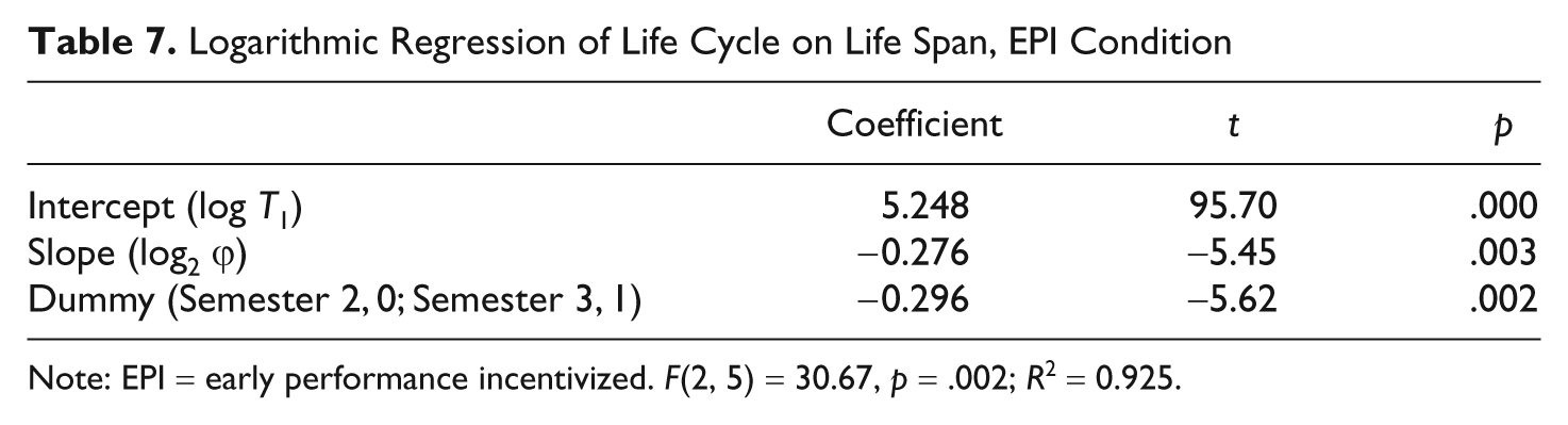
Note: EPI = early performance incentivized. F(2, 5) = 30.67, p = .002; R² = 0.925.

Conclusion

As hypothesized, participants responded rationally to differences in incentive conditions, attesting to the workability of incorporating multiple life cycles into a computer-assisted business gaming simulation. When early completion was incentivized, the majority of those who completed more than two life cycles improved their performance in subsequent life cycles, but a substantial minority did not. This suggests that, for a substantial minority, the incentive for early performance may have had a detrimental effect on learning—they may have choked under pressure. Although the pedagogically ideal solution should be to apply the EPI condition to the majority, so that their time is not wasted waiting for their slower colleagues, and to apply the EPA condition to the minority, so as to nurture their learning, the ideal may be impractical for the usual college setting. The more practical solution may to be set conditions that suit the majority and to mitigate its deleterious effects on the minority by gentle encouragement.

This study measured learning in a different way from those of many other studies supportive of business simulations, but its finding that participants learn from business simulations is consistent with those other studies. This study’s contribution to the literature on learning from business simulations is to present a behavioral method of measuring that learning and supply a numerical estimate of the learning rate for comparative studies.

The learning rate for the simulation used in this study was estimated at 17.4% for every doubling of experience. The rate is associated with a computer-assisted simulation, one of a design that is characteristically different from the computer-based and computer-controlled simulations more commonly used in business schools (Faria & Wellington, 2004) and industrial training programs (Summers, 2004). In laying out their four-quadrant typology of computer-mediated simulations Crookall et al. (1986) assert that:

in terms of learning possibilities, the [computer-assisted simulation] will have greater scope and potential than other types when social and socially-mediated processes and skills are seen as important learning outcomes. (p. 370)

If greater potential and scope implies a higher learning rate, then this study provides a basis for testing the assertion.

Moreover, measuring the learning rate should enable simulation developers and administrators to assess the effectiveness of features and ancillary activities. Features that raise the learning rate would be desirable, because it would make learning less dependent on the vagaries of context. Thus, periodic debriefings (Peters & Vissers, 2004) may raise the learning rate substantially, as it apparently did in a simpler exercise (Qudrat-Ullah, 2007). This and other ancillary activities remain to be evaluated for their possible contributions to the business simulation experience.

Footnotes

Acknowledgements

I would like to thank the anonymous reviewers for many helpful comments.

The author declared no potential conflicts of interest with respect to the authorship and/or publication of this article.

The author received no financial support for the research and/or authorship of this article.

Bio

Precha Thavikulwat is professor of management at Towson University and a fellow and past president of the Association for Business Simulation and Experiential Learning. His research interest is in the design of computerized business gaming simulations, especially for the purpose of assessing business education. He is the author of four computerized business gaming simulations: MANAGEMENT 500, CEO, DEAL, and GEO. Contact: pthavikulwat@towson.edu.

References

Anderson

P. H.

Lawton

(1992a). A survey and methods used for evaluating student performance on business simulations. Simulation & Gaming: An Interdisciplinary Journal, 23, 490-498.

Anderson

P. H.

Lawton

(1992b). The relationship between financial performance and other measures of learning on a simulation exercise. Simulation & Gaming: An Interdisciplinary Journal, 23, 326-340.

Anderson

P. H.

Lawton

(2009). Business simulations and cognitive learning: Developments, desires, and future directions. Simulation & Gaming: An International Journal, 40, 193-216.

Andress

F. J.

(1954, January-February). The learning curve as a production tool. Harvard Business Review, 32, 87-97.

Ariely

Gneezy

Loewenstein

Mazar

(2009). Large stakes and big misktakes. Review of Economic Studies, 76, 451-469.

Baumeister

R. F.

(1984). Choking under pressure: Self-consciousness and paradoxical effects of incentives on skillful performance. Journal of Personality and Social Psychology, 46, 610-620.

Biggs

W. D.

(1990). Introduction to computerized business management simulations. In Gentry

J. W.

(Ed.), Guide to business gaming and experiential learning (pp. 23-35). East Brunswick, NJ: Nichols.

Campbell

D. T.

Stanley

J. C.

(1963). Experimental and quasi-experimental designs for research. Chicago, IL: Rand McNally.

Chiesl

N. E.

(1990). Interactive real time simulation. In Gentry

J. W.

(Ed.), Guide to business gaming and experiential learning (pp. 141-158). East Brunswick, NJ: Nichols.

10.

Crookall

Martin

Saunders

Coote

(1986). Human and computer involvement in simulation. Simulation & Games: An Interdisciplinary Journal, 17, 345-375.

11.

Demiashkevich

(1935). An introduction to the philosophy of education. New York, NY: American Book.

12.

Dewey

(1938). Experience and education. New York, NY: Macmillan.

13.

Dewey

(1944). Democracy and education. New York, NY: Free Press.

14.

Faria

A. J.

Wellington

W. J.

(2004). A survey of simulation game users, former-users, and never-users. Simulation & Gaming: An International Journal, 35, 178-207.

15.

Fritzsche

D. J.

Cotter

R. V.

(1990). Guidelines for administering business games. In Gentry

J. W.

(Ed.), Guide to business gaming and experiential learning (pp. 253-278). East Brunswick, NJ: Nichols.

16.

GEO. (2006). [Developed by P. Thavikulwat]. Towson, MD. Retrieved from http://pages.towson.edu/precha/geo

17.

Goosen

K. R.

Jensen

Wells

(2001). Purpose and learning benefits of simulations: A design and development perspective. Simulation & Gaming: An International Journal, 32, 21-39.

18.

Gosen

Washbush

(2004). A review of scholarship on assessing experiential learning effectiveness. Simulation & Gaming: An International Journal, 35, 270-293.

19.

Hirschmann

W. B.

(1964, January-February). Profit from the learning curve. Harvard Business Review, 42, 125-139.

20.

Jonassen

D. H.

(2003). The vain quest for a unified theory of learning. Educational Technology, 43, 5-8.

21.

Keys

(1987). Total enterprise business games. Simulation & Gaming: An Interdisciplinary Journal, 18, 225-241.

22.

Keys

(1997). Strategic management games: A review. Simulation & Gaming: An Interdisciplinary Journal, 28, 395-422.

23.

Peters

V. A.

Vissers

G. A.

(2004). A simple classification model for debriefing simulation games. Simulation & Gaming: An International Journal, 35, 70-84.

24.

Pillutla

(2003). Creating a Web-based simulation gaming exercise using PERL and JavaScript. Simulation & Gaming: An International Journal, 34, 112-130.

25.

Qudrat-Ullah

(2007). Debriefing can reduce misperceptions of feedback: The case of renewable resource management. Simulation & Gaming: An International Journal, 38, 382-397.

26.

Reguero

(1957). An economic study of the military airframe industry. Wright-Patterson Air Force Base, OH: Department of the Air Force.

27.

Rollier

(1992). Observations of a corporate facilitator. Simulation & Gaming: An Interdisciplinary Journal, 23, 442-456.

28.

Summers

(2004). Today’s business simulation industry. Simulation & Gaming: An International Journal, 35, 208-241.

29.

Teach

(1993). Forecasting and management ability: A response to Wolfe. Simulation & Gaming: An Interdisciplinary, 24, 63-72.

30.

Thavikulwat

(1990). Consumption as the objective in computer-scored total enterprise simulations. Developments in Business Simulation & Experiential Exercises, 17, 167-169.

31.

Thavikulwat

(1996). Activity-driven time in computerized gaming simulations. Simulation & Gaming: An Interdisciplinary Journal, 27, 110-122.

32.

Thavikulwat

(1997). Real markets in computerized top-management gaming simulations designed for assessment. Simulation & Gaming: An Interdisciplinary Journal, 28, 276-285.

33.

Thavikulwat

(2004). The architecture of computerized business gaming simulations. Simulation & Gaming: An International Journal, 35, 242-269.

34.

Thavikulwat

Pillutla

(2008). Pure and mixed strategies for programmed trading in a periodic double auction. International Journal of Applied Decision Sciences, 1, 338-358.

35.

Washbush

Gosen

(2001). An exploration of game-derived learning in total enterprise simulations. Simulation & Gaming: An International Journal, 32, 281-296.

36.

Wolfe

(1990). The evaluation of computer-based business games: Methodology, findings, and future needs. In Gentry

J. W.

(Ed.), Guide to business gaming and experiential learning (pp. 279-300). East Brunswick, NJ: Nichols.

37.

Wolfe

(1997). The effectiveness of business games in strategic management course work. Simulation & Gaming: An Interdisciplinary Journal, 28, 360-376.

38.

Wolfe

Castroviovanni

(2006). Business games as strategic management laboratories. Developments in Business Simulation & Experiential Learning, 33, 31-40.

39.

Wolfe

Rogé

N. R.

(1997). Computerized general management games as strategic management learning environments. Simulation & Gaming: An Interdisciplinary Journal, 28, 423-441.

40.

Wright

T. P.

(1936). Factors affecting the cost of airplanes. Journal of the Aeronautical Sciences, 3, 122-128.