A quasi-static algorithm that includes effects of characteristic time scales for simulating failures in brittle materials

Abstract

When the brittle heterogeneous material is simulated via lattice models, the quasi-static failure depends on the relative magnitudes of $T_{elem}$ , the characteristic releasing time of the internal forces of the broken elements and $T_{lattice}$ , the characteristic relaxation time of the lattice, both of which are infinitesimal compared with $T_{load}$ , the characteristic loading period. The load–unload (L–U) method is used for one extreme, T_elem ≪ T_lattice, whereas the force–release (F–R) method is used for the other, T_elem ≫ T_lattice. For cases between the above two extremes, we develop a new algorithm by combining the L–U and the F–R trial displacement fields to construct the new trial field. As a result, our algorithm includes both L–U and F–R failure characteristics, which allows us to observe the influence of the ratio of $T_{elem}$ to $T_{lattice}$ by adjusting their contributions in the trial displacement field. Therefore, the material dependence of the snap-back instabilities is implemented by introducing one snap-back parameter γ. Although in principle catastrophic failures can hardly be predicted accurately without knowing all microstructural information, effects of γ can be captured by numerical simulations conducted on samples with exactly the same microstructure but different γs. Such a same-specimen-based study shows how the lattice behaves along with the changing ratio of the L–U and F–R components.

Keywords

Characteristic time scale quasi-static failure force–release load–unload lattice modeling elemental failure sequence displacement-controlled loading snap-back instability

Introduction

The focus of our work is to develop a new algorithm to simulate quasi-static failures that are beyond the reaches of the existing methods.

From the physics of quasi-static failures, different brittle materials have different degrees of snap-back instability in avalanche (Liu and El Sayed, 2011; Rinaldi and Lai, 2007; Rong et al., 2006). The term ‘snap back’ is meant as a cascade of ruptures of many links in correspondence of the same controlled displacement value in the displacement-controlled process (Rinaldi and Lai, 2007). ‘Links’ are simply lattice elements when it comes to lattice models. However, neither the force–release (F–R) method nor the load–unload (L–U) method has the ability to adjust the material-dependent snap-back instability: for existing lattice models of heterogeneous brittle materials, the failure behavior is completely determined by Young’s moduli, Poisson’s ratios and elastic strength limits of different phases and the geometrical microstructures. To describe the failure in a more accurate manner, there is a need to establish an algorithm with consideration of the snap-back properties.

Reflection on the F–R and L–U methods from the viewpoint of characteristic time scales

Quasi-static failures of heterogeneous media such as rocks and concrete have been numerically simulated repeatedly by lattice models (Karihaloo et al., 2003; Krajcinovic and Vujosevic, 1998; Liu et al., 2007, 2008a, 2009a, 2009b; Li et al., 2002; Ostoja-Starzewski, 2002). However, the term ‘quasi-static’ is paradoxical. In a lattice based on the equivalence of the strain energy (Karihaloo et al., 2003; Liu et al., 2007), if the loading rate is infinitely slow, indicating that T_load ≫ T_elem and T_load ≫ T_lattice, it is not difficult for the elastic response without any lattice elemental failure to get close to the ‘static solution’. However, once elemental deletions or equivalently microdamages begin, the actual physical process is definitely not in equilibrium and therefore not likely to be ‘static’. The term ‘quasi-static’ at this stage should therefore be understood in a loose sense. Namely the ‘quasi-static’ failure is composed of a series of equilibrium states among which between every adjacent two is one nonequilibrium process. Comparison of characteristic time scales is important in such a trans-scaled coupling problem because the rate processes at the two levels can compete with each other by their characteristic time scales although the ratio of mesoscopic to macroscopic length scales is infinitesimal (Bai et al., 2002, 2005). For example, Barenblatt (1993) emphasizes the significance of the Deborah number, D_e, defined as the ratio of the characteristic relaxation time of a mesoscopic process to the corresponding imposed macroscopic time scale. One important effect due to such time-scale competitions is the variation in the snap-back instability.

As all quasi-static failure algorithms have done (for instance, Bolander and Saito, 1998; Elias et al., 2010; Herrmann and Roux, 1992; Karihaloo et al., 2003; Liu et al., 2007; Rinaldi et al., 2008; Rots et al., 2008), if we still try to simulate these nonequilibrium processes between successive equilibrium states in the ‘quasi-static’ framework, a proper ‘quasi-static’ assumption becomes indispensable. In principle, innumerable quasi-static failure assumptions can be made. However, one assumption can become meaningful only if it is based upon physical characteristics of failure processes, or more particularly relative magnitudes of characteristic time scales, $T_{load}, T_{lattice}$ and $T_{elem}$ . Correspondingly, these are the following three categories (Liu and El Sayed, 2011):

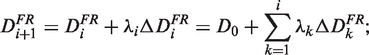
Case 1. T_load ≫ T_elem ≫ T_lattice. In this case, the release of the internal forces in ruptured elements is infinitely slower than the relaxation of the lattice. For example, take a lattice system in which each broken spring is connected in parallel with a dashpot whose viscosity coefficient is very large. In other words, such a slow release of internal forces in the ruptured element leads to a considerable dependence of failure processes on the elemental failure sequence. It is generally simulated by the F–R method (Elias et al., 2010; Liu, 2007; Liu et al., 2009b, 2010a). A trial displacement field is constructed to be compatible with the controlled displacements throughout the failure process, including non-equilibrium processes between successive equilibrium states. The elemental internal forces to be released are regarded as static actions, which are supposed to release from the initial value to zero. Thus, based on the principle of superposition (Fung, 1993), the sequence of the induced failures can be traced successively. The main characteristic of this method is that the forces to be released are applied in a straightforward manner to the system during the induced failure process, say the nonequilibrium avalanche between successive equilibrium states without the need to introduce any explicit elemental stiffness evolution (Liu and El Sayed, 2011). The F–R method can only produce vertical drop instead of snap-back. The avalanche process is simplified as the vertical drop of the reaction force under certain level of controlled displacement (Rinaldi, 2009; Rinaldi and Lai, 2007). This feature will be shown in ‘An illustrative example’ section.

Case 2. T_load ≫ T_lattice ≫ T_elem. The relaxation of the lattice is infinitely slower than the release of internal forces of ruptured elements. As discussed in Liu and El Sayed (2011), the elemental failure sequence can be neglected when checking the existence of induced failures. Due to this particular physical feature, the L–U method is more accurate than the F–R method. It is notable that ‘unload’ here does not mean plastic unloading but rather the removal of external elastic loading. Lattices are composed of linear-elastic line elements like bars or beams among which a strength criterion is adopted for each. The L–U method can be summarized as follows (Herrmann and Roux, 1992; Karihaloo et al., 2003; Rinaldi and Lai, 2007; Rots et al., 2008; van Mier et al., 2002). The load is applied gradually and a linear elastic analysis is performed until the element which is the aptest to break reaches its strength limit. This particular element is then eliminated and a new analysis is performed. The stiffness matrix is updated while keeping the applied load unchanged to check whether another element will fail. If no more elements fail, the calculation is restarted from zero loads again until the specimen completely fails. The L–U method becomes reasonable when T_elem ≪ T_lattice ≪ T_load, which is the quasi-static assumption hidden behind the L–U method. The L–U method can predict the upper limit of the snap back instability, as will be shown in ‘An illustrative example’ section.

Case 3. T_load ≫ T_lattice ≫ T_elem. The relaxation of the lattice is approximately as quick as the release of the internal forces of the ruptured elements. For this case, both the F–R method and the L–U method will not work well. The snap-back instability is between the F–R vertical drop and the L–U (upper) limit, and varies with the relative magnitudes of $T_{lattice}$ and $T_{elem}$ . If we say that the viscosity coefficient is almost infinite in Case 1 and nearly zero in Case 2, the method proposed in this study aims to describe the failure behaviors in between. The equilibrium conditions are satisfied in this new method, as will be illustrated in ‘An illustrative example’ section.

Highlight of the new algorithm

As explained in the previous section, both the F–R and L–U methods will not work well in simulating ‘Case 3’ because of the lack of ability to consider degrees of snap-back instability; a new methodology is required.

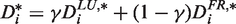
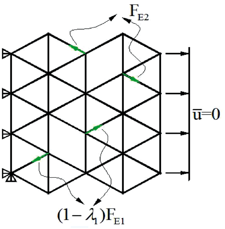
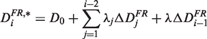
In fact ‘Case 3’ represents a large collection between ‘Case 1’ of the extreme of T_elem ≫ T_lattice and ‘Case 2’ of the extreme of T_lattice ≫ T_elem. Since the F–R and L–U methods are respectively used for these two extremes, we argue that the cases in between can be simulated by combining these two methods together. The key difference between F–R and L–U lies in the trial displacement fields used to check possible induced failures. Therefore, the new trial displacement field is assumed to be a linear interpolation of the F–R field and the L–U one

D_{i}^{*} = γ D_{i}^{LU, *} + (1 - γ) D_{i}^{FR, *}

(1)

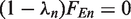
where the displacement fields with superscript ‘*’ are the trial ones, while fields without it denote equilibrium ones. The subscript ‘i’ is the sequential numbering of failures within an avalanche process between two successive equilibrium states, which will be shown in more details in the following sections. γ is considered to be related to

R = \frac{T_{elem}}{T_{lattice}}

and has the following characteristics

\begin{matrix} γ = {\begin{matrix} 1 & R = R^{LU} \to 0 \\ γ (R) \in (0, 1) with \frac{\partial γ}{\partial R} < 0 & R^{LU} < R < R^{FR} \\ 0 & R = R^{FR} \to \infty \end{matrix} \end{matrix}

(2)

indicating that γ controls the proportions of the F–R trial field,

D_{i}^{FR, *}

, and the L–U trial field,

D_{i}^{LU, *}

, in the combined trial displacement field,

D_{i}^{*}

, where

R^{LU}

and

R^{FR}

are R-values respectively when T_elem≪ T_lattice and when T_elem ≫ T_lattice.

Here, γ is a material property instead of simply a numerical-interpolation factor that lacks a physical meaning because γ is related to the characteristic time scales which are material-dependent.

Additionally, it is worth pointing out that rationality of algorithms for simulating quasi-static failures should also be checked based on the γ-value, or equivalently the characteristic time scales mentioned above. Elias et al. (2010) conclude that the secant solution scheme which is equivalent to the L–U method is not proper for non-proportional loading, then suggest that the F–R method is a more robust scheme. Unfortunately, this is only true for the F–R extreme. A systematic comparison is recently made by Liu and El Sayed (2011), concluding that F–R and L–U methods are actually for different-featured physics processes and therefore it is meaningless to say which is absolutely better than the other.

Article structure

The remainder of this article is organized as follows. In the following sections, the L–U method and the F–R method are respectively revisited, in order to make convenient the presentation of the new algorithm combining the F–R and L–U methods together in section ‘A new algorithm combining the L-U and F-R methods’, where a simple specially designed 1D tensile test is also provided for a clear demonstration. Numerical examples are conducted in the later section to show our algorithm’s capacity to capture at least qualitative effects of characteristic time scales. Conclusions are presented in the last section.

The L–U method

The L–U method becomes applicable when T_load ≫ T_lattice ≫ T_elem (Liu and El Sayed, 2011).

Without loss of generality, a bar-lattice system is chosen where the bar can only sustain tensile/compressive loadings. In this article, the bar is ideally linearly elastic and totally loses its load-bearing capability once its strength limit is reached. As a result, the stiffness matrix of the lattice system is obtained by simply assembling elemental stiffness matrices of all intact bar elements in the system.

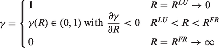
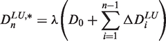
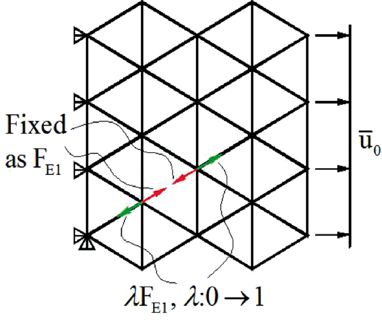
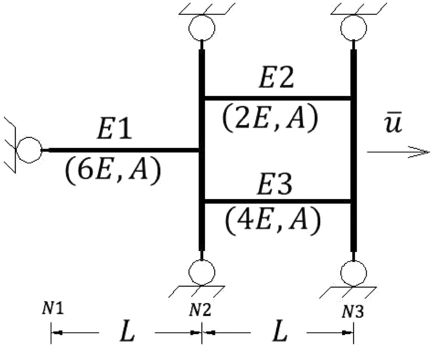
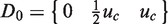
Under quasi-static monotonic increasing controlled displacement, $\bar{u}$ , as shown in Figure 1 and as the load reaches the value ${\bar{u}}_{0}$ , element E1 firstly reaches its strength limit $u_{c}^{E 1}$ and needs to be eliminated. The displacement field at this moment is written as D₀ and the internal force in E1 is $F_{E 1}$ . Then, E1 is deleted from the lattice system and the same external controlled displacement ${\bar{u}}_{0}$ is applied to the updated system to check whether other element(s) will fail. The trial displacement field under these conditions is represented by $D_{2}^{LU, *}$ . From this point forward, we will call the first induced elemental failure the ‘first-order induced failure’, and the corresponding element is called the ‘first-order induced element’.

Figure 1.

Boundary and loading conditions for a displacement-controlled tensile test on a lattice.

In order to determine the relationship between $D_{2}^{LU, *}$ and D₀, we need to refer to the L-U quasi-static assumption, T_load ≫ T_lattice ≫ T_elem, indicating that the relaxation of the lattice is infinitely slower than the release of the internal forces of the ruptured elements. This way, the sequence of previous elemental failures can be neglected in predicting the upcoming induced failure. In other words, at this particular controlled-displacement level, all existing failures, including the initial failure and all consequential induced failures, can be assumed to happen simultaneously when detecting the existence of further induced failure. Briefly, when checking the occurrence of the nth-order rupture, elements E i $(i = 1, 2, \dots, n - 1)$ having ruptured previously can be assumed to break simultaneously, such that the elemental failure sequence is neglected, namely

D_{n}^{LU, *} = λ (D_{0} + {\sum^{n - 1}}_{i = 1} Δ D_{i}^{LU})

(3)

where

Δ D_{i}^{LU}

is the incremental displacement field caused by the fully released internal force in E i, which is calculated under the following conditions: the controlled displacement is set to zero, the ith ruptured element is removed from the specimen but its internal force is applied onto their ends in the opposite directions. More details on the calculation of

Δ D_{i}^{LU}

can be found in (Liu and El Sayed, 2011). It deserves making clear that in cases where two or more bar elements are induced to break simultaneously, due to the nature of T_load ≫ T_lattice ≫ T_elem, the contribution of each bar rupture is independently considered as

Δ D_{i}^{LU}

, and the failure sequence does not matter. In other words, it does not matter whether bars break simultaneously or sequentially. It is notable that when no more bars get broken under the controlled displacement

\bar{u}, λ

in equation (3) should be equal to 1, therefore now equation (3)

D_{n}^{LU} = D_{n}^{LU, *} = D_{0} + {\sum^{n - 1}}_{i = 1} Δ D_{i}^{LU}

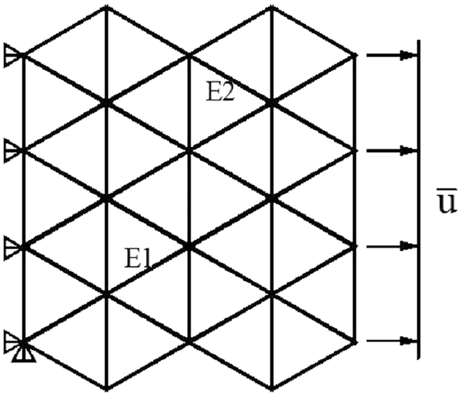
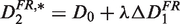
For example, if there are no more elements reaching their strength limits after the breakage of E1 at the load level

{\bar{u}}_{0}

, as shown in Figure 2, we have

D_{2}^{LU} = D_{0} + Δ D_{1}^{LU}

(4)

Actually, equation (3) has already indicated that the sequence of currently

n - 1

existing failures is not included. That is, among these

n - 1

failures, E i failing before E j, or E j failing before E i makes no difference to the trial displacement field

D^{LU}

Figure 2.

Relationship among deforming fields based on the principle of superposition.

The F–R method

This method can be employed to simulate quasi-static failures when T_load ≫ T_elem ≫ T_lattice (Elias et al., 2010; Liu, 2007; Liu and El Sayed, 2011; Liu et al., 2009b).

It is established based on the following equivalent transformation. As shown in Figure 3, the contribution of element E1 to the rest of the system is to apply a force, $F_{E 1}$ , to both of its ends in opposite directions. Apparently, if E1 is eliminated from the system while its actions remain active, the remaining system will maintain exactly the same deformation state as before removing E1.

Figure 3.

Two equivalent forms of the same displacement field D₀.

Following the example studied in the ‘The L–U method’ section, a new way to construct the trial displacement field is introduced according to the principle of superposition (Fung, 1993). Once E1 reaches its strength limit, the process of deleting it can be considered as the decrease in the actions labeled with red arrows in Figure 3 from $F_{E 1}$ to 0. Here, for the sake of computational convenience, we implement it in a different way: as shown in Figure 4, we keep the red actions unchanged as $F_{E 1}$ and apply a new pair of actions (labeled with green arrows) on the system at both ends of E1.

Figure 4.

Displacement field $D_{2}^{FR, *} = D_{0} + λ Δ D_{1}^{FR}$ , where $λ F_{E 1}$ is the part already released among the initial value, $F_{E 1}$ .

Thus, another equivalent relation appears – the decrease in the red action pair from $F_{E 1}$ to 0 corresponds to the increase in the green action pair from 0 to $F_{E 1}$ . Both denote the same process, namely the stress redistribution due to the release of the internal force in E1. The resultant action of the green and red pairs is the amount of the internal force remaining in E1 to be released. The trial displacement field in this releasing process can be summarized as (Figure 4)

D_{2}^{FR, *} = D_{0} + λ Δ D_{1}^{FR}

where λ has a robust physical meaning, namely the degree to which E1’s internal force has been released;

λ = 1

corresponds to the force being completely released. Let

λ_{1}

denote the value when the first-order induced element E2 reaches its strength limit. At this moment, E2’s internal force is denoted as

F_{E 2}

, and correspondingly we have

The displacement field: $D_{2}^{FR} = D_{0} + λ_{1} Δ D_{1}^{FR}$ ;

The force to be released at E1’s ends: $(1 - λ_{1}) F_{E 1}$ ;

The force to be released at E2’s ends: $F_{E 2}$ .

The next task is to check whether another element would be induced to fail due to the release of both $(1 - λ_{1}) F_{E 1}$ at E1’s ends and $F_{E 2}$ at E2’s ends. The trial displacement field is

D_{3}^{FR, *} = D_{2}^{FR} + λ Δ D_{2}^{FR} = D_{0} + λ_{1} Δ D_{1}^{FR} + λ Δ D_{2}^{FR} (0 < λ < 1)

(5)

where

Δ D_{2}^{FR}

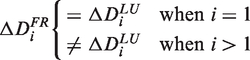
is calculated as shown in Figure 5. It is notable that

\begin{matrix} Δ D_{i}^{FR} {\begin{matrix} = Δ D_{i}^{LU} & when i = 1 \\ \neq Δ D_{i}^{LU} & when i > 1 \end{matrix} \end{matrix}

Once induced failures begin, they become different because the L–U method has nothing to do with the sequence of induced failures, but the F–R method does. Again, we emphasize that we should consider the subscript “i” in the above relation as the order number of induced failure (ith-order induced failure) instead of the numbering of induced elements because the ith-order induced failure can be composed of two or more elements induced to break simultaneously.

Figure 5.

Boundary and loading conditions for obtaining $Δ D_{2}^{FR}$ .

The appearance of further induced failure, i.e. the second-order induced failure, indicates that there exists a special value, $λ_{2}$ , at which the second-order induced failure happens in element E3. We thus have

The displacement field:

D_{3}^{FR} = D_{0} + λ_{1} Δ D_{1}^{FR} + λ_{2} Δ D_{2}^{FR}

(6)

The force to be released at E1’s ends: $(1 - λ_{2}) [(1 - λ_{1}) F_{E 1}] = (1 - λ_{1}) (1 - λ_{2}) F_{E 1}$ ;

The force to be released at E2’s ends: $(1 - λ_{2}) F_{E 2}$ ;

The force to be released at E3’s ends: $F_{E 3}$ .

…

When the ith-order induced failure happens, we would have the following:

The displacement field:

D_{i + 1}^{FR} = D_{i}^{FR} + λ_{i} Δ D_{i}^{FR} = D_{0} + {\sum^{i}}_{k = 1} λ_{k} Δ D_{k}^{FR};

(7)

where it is notable that a hidden relation under the current notations is

D_{1}^{FR} = D_{0}

which actually has already been indicated by Figure 3.

The force to be released at E1’s ends:

(1 - λ_{1}) (1 - λ_{2}) \dots (1 - λ_{i}) F_{E 1};

(8)

The force to be released at E2’s ends:

(1 - λ_{2}) (1 - λ_{3}) \dots (1 - λ_{i}) F_{E 2};

(9)

…

The force to be released at E i’s ends:

(1 - λ_{i}) F_{Ei};

(10)

The force to be released at E $(i + 1)$ ’s ends: $F_{E (i + 1)}$ .

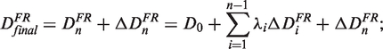
If we assume that the total number of induced failures is

n - 1

, then after the appearance of the

(n - 1)

th-order induced failure in element E n, the field will be driven by the forces left to be released in E1, E2, … , E n to the final equilibrium state corresponding to the loading level,

{\bar{u}}_{0}

. In this final state, the factor adjusting the field increment,

Δ D_{n}^{FR}

, is equal to 1, i.e.

λ_{n} = 1

, indicating that no more induced failure would occur. Hence,

The final equilibrium displacement field admissible in both the kinematic and strength conditions

D_{final}^{FR} = D_{n}^{FR} + Δ D_{n}^{FR} = D_{0} + {\sum^{n - 1}}_{i = 1} λ_{i} Δ D_{i}^{FR} + Δ D_{n}^{FR};

(11)

The force to be released at E1’s ends:

(1 - λ_{1}) \dots (1 - λ_{i}) \dots (1 - λ_{n - 1}) (1 - λ_{n}) F_{E 1} = 0;

(12)

The force to be released at E2’s ends:

(1 - λ_{2}) \dots (1 - λ_{i}) \dots (1 - λ_{n - 1}) (1 - λ_{n}) F_{E 2} = 0;

(13)

…

The force to be released at Ei’s ends:

(1 - λ_{i}) \dots (1 - λ_{n - 1}) (1 - λ_{n}) F_{Ei} = 0;

(14)

…

The force to be released at E n’s ends:

(1 - λ_{n}) F_{En} = 0

(15)

We can see that all the elements ruptured at the level

{\bar{u}}_{0}

have totally released their internal forces in

D_{final}^{FR}

as they are all to be multiplied by the factor

1 - λ_{n}

, which is equal to 0. Furthermore, when compared with the L–U method, here the internal forces to be released are considered as static actions; therefore, the releasing sequence becomes dominant in the failure propagation.

A new algorithm combining the L–U and F–R methods

As discussed in the introduction, we present a new algorithm to simulate quasi-static failures that are out of the reaches of both the L–U and F–R methods. Its main feature is to implement the material-dependence on the snap-back behaviors, or more particularly, the dependence on materials’ characteristic time scales.

Algorithm formula

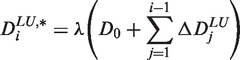
We propose a new algorithm for cases between the extremes T_elem ≫ T_lattice and T_lattice ≫ T_elem. Firstly, it is helpful to summarize the key points in both sections ‘The L–U method’ and The F–R method’. After the breakage of the $(i - 1)$ -th element and to judge the occurrence of the i-th failure element, the trial displacement field used in the L–U method is written according to equation (3) as

D_{i}^{LU, *} = λ (D_{0} + {\sum^{i - 1}}_{j = 1} Δ D_{j}^{LU})

(16)

From equation (7), the F–R counterpart is

D_{i}^{FR, *} = D_{0} + {\sum^{i - 2}}_{j = 1} λ_{j} Δ D_{j}^{FR} + λ Δ D_{i - 1}^{FR}

(17)

Then, as briefly mentioned in the introduction, we construct a new kind of trial displacement field in the form

D_{i}^{*} = γ D_{i}^{LU, *} + (1 - γ) D_{i}^{FR, *}

(18)

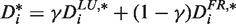
where γ has the qualitative characteristics shown in equation (2) and reflects the snap-back properties of materials which will be demonstrated in the upcoming examples. Substitution of equations (16) and (17) into equation (18) yields

\begin{matrix} D_{i}^{*} = (1 - γ) [D_{0} + {\sum^{i - 2}}_{j = 1} λ_{j} Δ D_{j}^{FR}] + λ [(1 - γ) Δ D_{i - 1}^{FR} + γ (D_{0} + {\sum^{i - 1}}_{j = 1} Δ D_{j}^{LU})] \\ = {D^{base}}_{i} + λ Δ D_{i - 1} \end{matrix}

(19)

from which we can easily find that

D_{i}^{*} = D_{i}^{LU, *}

when

γ = 1

, while

D_{i}^{*} = D_{i}^{FR, *}

when

γ = 0

. For

γ \in (0, 1), D_{i}^{*}

is the linear combination of

D_{i}^{LU, *}

and

D_{i}^{FR, *}

. Since

D_{0}, Δ D_{j}^{LU}

and

Δ D_{j}^{FR} (j = 1, 2, \dots, i - 1)

are all equilibrium fields. The trial field

D_{i}^{*}

in equation (19) is also an equilibrium one. We argue that the trial displacement field,

D_{i}^{*}

, in equation (19) simultaneously has two characteristics: (1) that of the L–U extreme, T_lattice ≫ T_elem, corresponding to the relative share γ; and (2) that of the F–R extreme, T_elem ≫ T_lattice, corresponding to the relative share

1 - γ

. Therefore, by adjusting the γ-value, the relative magnitudes of

T_{elem}

and

T_{lattice}

are changed. This way, the present method is expected to have the capability of predicting failure responses of lattices with various micro-level characteristic time scales

T_{elem}

and macro-level characteristic time scales,

T_{lattice}

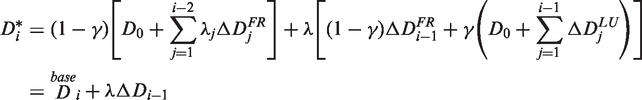
It is worthwhile to introduce the concept of the ‘base displacement field’ as shown in equation (19), i.e.

{D^{base}}_{i} = (1 - γ) [D_{0} + {\sum^{i - 2}}_{j = 1} λ_{j} Δ D_{j}^{FR}]

(20)

defining the ‘base state’ from which further induced failures should be checked. Actually, such a γ-related base displacement field leads to different snap-back degrees during an avalanche. When

γ = 1

, the snap-back behavior occurs to the maximum extent. When

γ = 0

, it changes to the vertical drop like what happens in the case of T_elem ≫ T_lattice and no snap-back can happen.

An illustrative example

A simple example is given to show the relationships among $γ, {D^{base}}_{i}$ and the snap-back characteristic. This way, relationships among the L–U method, the F–R method and the present one are explored. The advantage of the present algorithm as a more general approach is illustrated. Its ability to implement the material-dependence of the snap-back property is also emphasized.

The specially designed test is shown in Figure 6. Three 1D truss elements, E1, E2 and E3, are included. E2 and E3 are installed between two parallel rigid platens, resulting in E2 and E3 having the same elongation in the process. Their Young’s moduli are, respectively, $6 E, 2 E$ and $4 E$ . They have the common initial cross-section area A and the common initial length L. Their tensile strength limits are respectively $u_{c}, (\frac{1}{2} + δ) u_{c}$ and $\frac{1}{2} u_{c}$ , where _δ ≪ 1 is used only to differentiate the tensile strengths of E2 and E3 (namely, their failure sequences). In the following, except that we need tell the failure sequence, we adopt the approximation $\frac{1}{2} + δ \overset{\cdot}{=} \frac{1}{2}$ . Here, the strength limit means that, for example, when E1’s elongation reaches u_c, E1 will totally break. u_c has the dimension of length and satisfies the condition u_c ≪ L within the infinitesimal deformation framework. The specimen has three degrees of freedom, $u_{N 1} \equiv 0, u_{N 2}$ and $u_{N 3}$ , denoting the translational displacements of nodes N1, N2 and N3 along the direction of the controlled displacement $\bar{u}$ . Such a specially designed example is inspired by the parallel-bar system (PBS) as a damage model used in Krajcinovic et al. (1993). PBS is a simple but efficient methodology to study damage revolutions. It is also notable that the snap-back instability has not been considered by Krajcinovic et al. (1993). Therefore, this study indicates extended applications of PBS-type analyses.

Figure 6.

The setup for the specially designed 1D tensile test.

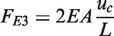
A 1D tensile test is conducted by applying controlled displacement $\bar{u}$ . When $\bar{u} = u_{c}$ , E3 reaches its tensile strength limit $\frac{1}{2} u_{c}$ . Note that now E2 is very close to its limit $(\frac{1}{2} + δ) u_{c}$ but still has not reached it. Therefore, now only E3 begins breaking. Corresponding to the onset of E3’s breakage, the displacement field is

D_{0} = {\begin{matrix} 0 & \frac{1}{2} u_{c} & u_{c} \end{matrix}}

(21)

where the three components of vector D₀ are, respectively, the displacements of nodes N1, N2 and N3, namely

u_{N 1} (D_{0}), u_{N 2} (D_{0}) and u_{N 3} (D_{0})

. In field D₀, the internal force of E3 is

F_{E 3} = 2 EA \frac{u_{c}}{L}

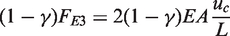
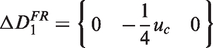
Since the share of the F–R field in the total field is

(1 - γ)

as shown in equation (18) and the concept of force release is limited only to the F–R method, the amount of internal force to be released in the combined trial field in defined equation (18) is

(1 - γ) F_{E 3} = 2 (1 - γ) EA \frac{u_{c}}{L}

(22)

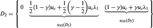
According to equation (19), the field on the existence of further failures induced by the breakage of E3 can be written as

D_{2} = (1 - γ) D_{0} + λ_{1} [(1 - γ) Δ D_{1}^{FR} + γ (D_{0} + Δ D_{1}^{LU})]

(23)

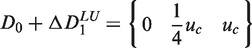
where D₀ is the field under controlled displacement

\bar{u} = u_{c}

on the specimen with three intact elements and has been given by equation (21).

Δ D_{1}^{FR}

is obtained by letting the controlled displacement

\bar{u} = 0

, deleting E3 and applying

F_{E 3}

on node N2 along the direction opposite to

\bar{u}

, and

F_{E 3}

on node N3 along the

\bar{u}

direction. By simple calculations of structural mechanics, we have

Δ D_{1}^{FR} = {\begin{matrix} 0 & - \frac{1}{4} u_{c} & 0 \end{matrix}}

(24)

while

D_{0} + Δ D_{1}^{LU}

should be obtained as a whole by deleting E3 and keeping

\bar{u} = u_{c}

and is given as

D_{0} + Δ D_{1}^{LU} = {\begin{matrix} 0 & \frac{1}{4} u_{c} & u_{c} \end{matrix}}

(25)

Substitution of equations (21), (24) and (25) into equation (23) yields

D_{2} = {\begin{matrix} 0 & {\underset{︸}{\frac{1}{2} (1 - γ) u_{c} + \frac{1}{2} (γ - \frac{1}{2}) u_{c} λ_{1}}}_{u_{N 2} (D_{2})} & {\underset{︸}{(1 - γ) u_{c} + γ u_{c} λ_{1}}}_{u_{N 3} (D_{2})} \end{matrix}}

(26)

If E2 is induced to break due to the breakage of E3, we know that the elongation of E2 should reach its limit

(\frac{1}{2} + δ) u_{c} \overset{\cdot}{=} \frac{1}{2} u_{c}

Δ l_{E 2} = u_{N 3} (D_{2}) - u_{N 2} (D_{2}) = \frac{1}{2} (1 - γ) u_{c} + \frac{1}{2} (γ + \frac{1}{2}) u_{c} λ_{1} \overset{\cdot}{=} \frac{1}{2} u_{c}

(27)

giving

λ_{1} \overset{\cdot}{=} \frac{2 γ}{2 γ + 1}

(28)

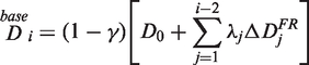
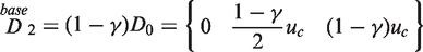
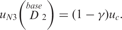
The base displacement field as defined in section ‘Algorithm formula’ now becomes

{D^{base}}_{2} = (1 - γ) D_{0} = {\begin{matrix} 0 & \frac{1 - γ}{2} u_{c} & (1 - γ) u_{c} \end{matrix}}

(29)

Note that the base displacement field indicates that the maximum snap-back state the specimen can reach, namely the possible minimum displacement of N3, is

u_{N 3} ({D^{base}}_{2}) = (1 - γ) u_{c} .

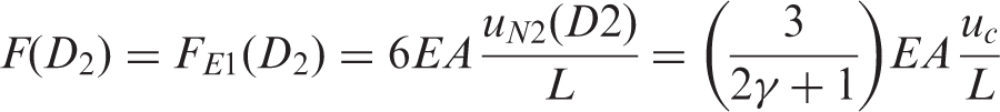
The reaction force sustained by the system is equal to E1’s internal force,

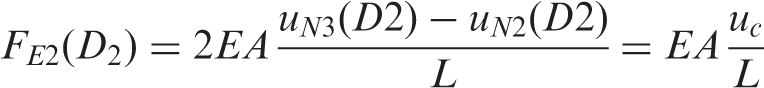
F (D_{2}) = F_{E 1} (D_{2}) = 6 EA \frac{u_{N 2} (D 2)}{L} = (\frac{3}{2 γ + 1}) EA \frac{u_{c}}{L}

(30)

while the internal force in E2 is

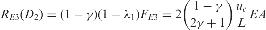
F_{E 2} (D_{2}) = 2 EA \frac{u_{N 3} (D 2) - u_{N 2} (D 2)}{L} = EA \frac{u_{c}}{L}

(31)

and the internal force of the breaking element, E3, remaining to be released is

R_{E 3} (D_{2}) = (1 - γ) (1 - λ_{1}) F_{E 3} = 2 (\frac{1 - γ}{2 γ + 1}) \frac{u_{c}}{L} EA

(32)

With the help of equations (30), (31) and (32), we get the following equation

R_{E 3} (D_{2}) + F_{E 2} (D_{2}) = F_{E 1} (D_{2})

(33)

which indicates that the displacement field D₂, as shown in equation (26), satisfies the equilibrium condition. In other words, D₂ denotes an equilibrium state. This characteristic shows that our newly constructed trial field is based on a reasonable quasi-static assumption.

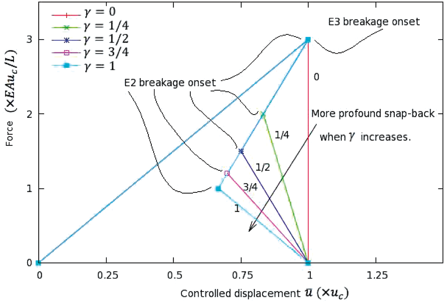
Now, we study the load-displacement, $P ~ \bar{u}$ diagram of the above failure process, as shown in Figure 7. This diagram is constructed by connecting the subsequent peaks, in a manner the same as used by van Mier and van Vliet (2003). For every particular γ value, this curve is composed of four points:

Point no. 1 $(P_{1}) - (0, 0),$ – corresponding to the origin.

Point no. 2 $(P_{2}) - (u_{c}, 3 EA \frac{u_{c}}{L})$ , corresponding to the moment when E3 reaches its limit.

Point no. 3 $(P_{3}) - (\frac{1 + γ}{1 + 2 γ} u_{c}, \frac{3}{2 γ + 1} EA \frac{u_{c}}{L})$ , corresponding to the moment when E2 reaches its limit.

Point no. 4 $(P_{4}) - (u_{c}, 0)$ , corresponding to the final state of complete failure of the specimen.

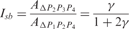
In the present example, for the purpose of making a quantitative comparison, the snap-back instability is calculated in the form

I_{sb} = \frac{A_{Δ P_{2} P_{3} P_{4}}}{A_{Δ P_{1} P_{2} P_{4}}} = \frac{γ}{1 + 2 γ}

(34)

where

A_{Δ P_{2} P_{3} P_{4}}

and

A_{Δ P_{1} P_{2} P_{4}}

are respectively the areas of the triangles

P_{2} P_{3} P_{4}

and

P_{1} P_{2} P_{4}

. From equation (34),

I_{sb}

increases along with increasing γ. Additionally, equation (34) does not mean that

I_{sb}

is only the function of γ and nothing else: it seems so because ratios of lengths, cross-section areas and moduli of bars have been replaced with their specific values. The area of the triangle

P_{2} P_{3} P_{4}

denotes the energy due to snap back. From this sense, a bigger

I_{sb}

value means a stronger snap back.

Figure 7.

Force–displacement curves with $γ = 0, \frac{1}{4}, \frac{1}{2}, \frac{3}{4}, 1$ .

Figure 7 shows the $P ~ \bar{u}$ diagrams for different γ values. We can find that the snap-back behavior is closely dependent on the γ-value. We take the following five γ values as examples:

$γ = 0$ : corresponding to the F-R result. The internal force of the breaking E3 is released infinitely slowly and no snap-back happens. Instead, during the induced failure process, the controlled displacement remains $\bar{u} = u_{c}$ , and the reaction force drops vertically. Since $δ \to 0$ , now E2 begins breaking almost simultaneously as E3 breaks. This case is the same as discussed by Liu et al. (2009a) and Elias et al. (2010).

$γ = \frac{1}{4}, \frac{1}{2}, \frac{3}{4}$ : As γ increases within the range $(0, 1)$ , the snap-back becomes more and more profound. A larger γ means a smaller force remaining to be released and therefore a lower reaction force level. From Figure 7, we can see that, at the point denoting the onset of E2’s breakage, the reaction force decreases as γ increases.

$γ = 1$ : corresponding to the L–U result. It is the upper limit of the snap-back behavior.

This simple 1D test indicates that the trial displacement field used to check the existence of induced failure(s) changes along with γ. This γ-dependence is expected to cause the difference in elemental failure sequences and therefore the final failure patterns, even though we have not shown this in this example, with a reason that the specially-designed one-dimensional parallel-bar system has difficulty in capturing the feather of changing failure sequence. It is expected that failure sequence will be scattered more easily by γ in a heterogeneous microstructure much more complex than the 1D PBS, which will be shown in the next section instead of here.

Numerical example and analysis

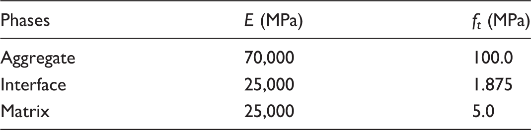
We study the failure patterns of a beam lattice under external quasi-static tensile controlled displacement with various γ-values:

γ = 0.0, γ = 0.5

and

γ = 1.0

. Here, the term ‘quasi-static’ means that T_load ≫ T_lattice and T_load ≫ T_elem. The beam lattice presented here is employed to describe the microstructures in particle composites such as concrete (Karihaloo et al., 2003; Liu et al., 2007, 2008b). The lattice material properties are listed in Table 1. In Table 1, we adopt critical tensile stress in order to keep consistent with those in literature. Nevertheless, it is notable that this study is limited to linear elastic problems, therefore the strength limits in terms of critical elongation, critical tensile stress and critical tensile force can easily be linked together through elemental geometrical parameters and elastic moduli.

Table 1.

The micro-elastic and strength properties of the phases.

Phases	E (MPa)	f_t (MPa)
Aggregate	70,000	100.0
Interface	25,000	1.875
Matrix	25,000	5.0

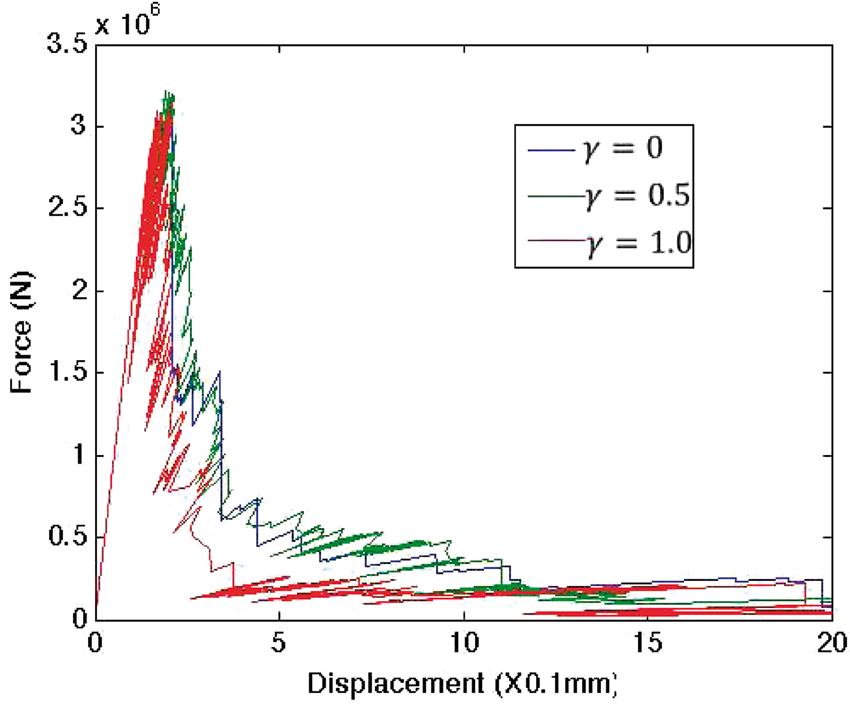
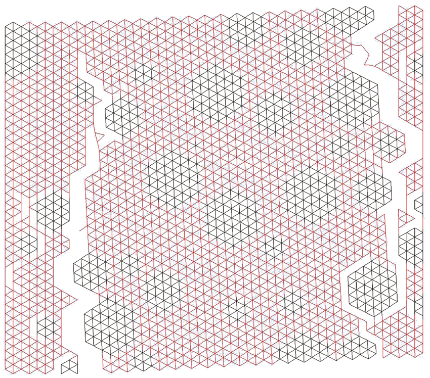
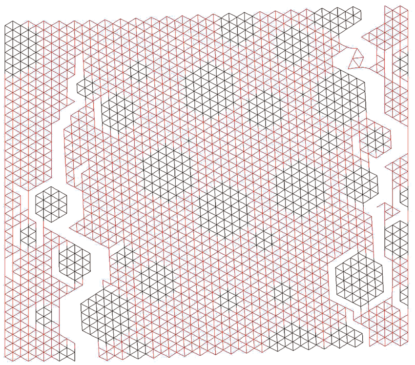
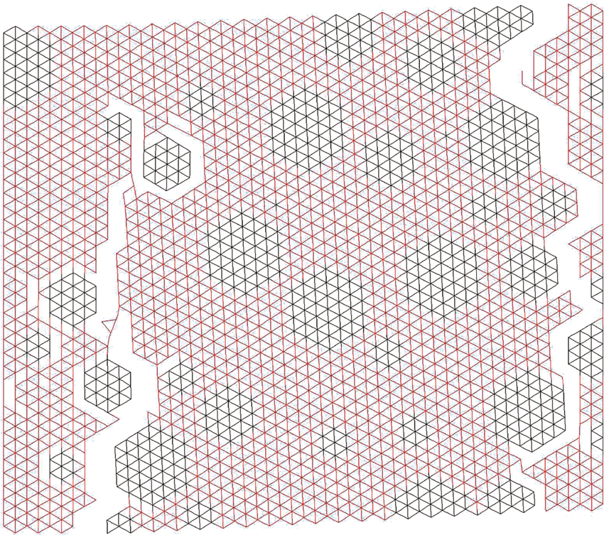
Figure 8 shows the force–displacement curves while Figures 9 –11 show the failure patterns when the controlled displacement is around 2.0 mm. Here, we emphasize that the final failure patterns depend significantly on γ, as mentioned in section ‘A new algorithm combining the L–U and F–R methods’. Here, the correct way to analyze the force–displacement curves in Figure 8 and the failure patterns in Figures 9 –11 is to imagine that significant differences can be expected to be caused by γ. One may say that the curves in Figure 8 show roughly the same tendency and therefore indicate roughly the same failure process, which is usually acceptable with the consideration of the statistical nature of the materials’ microstructures. Unfortunately, this does not work here because we employ specimens with exactly the same microstructures. It is well known that cracking behaviors of heterogeneous media such as concrete generally show significant degrees of randomness. Even though some statistical tendencies can be summarized based on finite numbers of experimental observations, such kinds of ‘statistical tendencies’ are never lack of exceptions. Heterogeneity of microstructure has been generally recognized as the dominant reason for this above scattering feature. Nevertheless, here it is further emphasized that effects of snap-back instability can make the cracking path among the heterogeneous structure even less determinate. Of course, snap-back instability is always combined together with microstructures to play its role. In one word, the purpose of this study is to show that the material-dependence of snap-back instability also scatters the cracking behavior, which is supported by differences among curves in Figure 8 and failure patterns in Figures 9 –11.

Figure 8.

Force–displacement curves when $γ = 0, 0.5, 1.0$ .

Figure 9.

The failure pattern when $\bar{u} = 2.0 mm$ and $γ = 0$ .

Figure 10.

The failure pattern when $\bar{u} = 2.0 mm$ and $γ = 0.5$ .

Figure 11.

The failure pattern when $\bar{u} = 2.0 mm$ and $γ = 1.0$ .

Conclusions

This article proposes a new algorithm to simulate quasi-static brittle failures that cannot be solved by either the L–U or F–R methods. In principle, this method is for cases between the L–U extreme, T_lattice ≫ T_elem and the F–R extreme, T_elem ≫ T_lattice. Of course, this new method is reduced to the L–U or F–R counterparts at these two extremes. As a result, it is a more general algorithm with a wider application range than both the L–U and F–R methods. It also has the implementation of adjustable material-dependent snap-back properties, which both the L–U and the F–R methods lack.

Here, we have introduced one parameter, γ, through which a new kind of trial displacement field is constructed by linearly combining the F–R field and the L–U field, to check the existence of further induced failures under the current level of controlled displacement, which satisfies the equilibrium conditions. γ has a physical meaning related to the ratio of characteristic time scales $T_{elem}$ and $T_{lattice}$ and should be taken as one material property indicator. The simple 1D tensile test in ‘A new algorithm combining the L–U and F–R methods’ section shows that the snap-back instability depends strongly on γ, namely the proportions of the F–R field and the L–U field in the total field. Our numerical example in the last section concludes that γ can also obviously change the failure patterns.

Footnotes

Acknowledgments

The authors would like to thank the reviewers for their valuable suggestions in improving the manuscript. They also thank Ms Lauratu Osul for her proofreading.

Conflict of interest

None declared.

Funding

This work was funded by the KAUST baseline fund.

References

Bai

Wang

Xia

(2005) Statistical mesomechanics of solid, linking coupled multiple space and time scales. Applied Mechanics Reviews, 58: 372–372.

Bai

Xia

(2002) Non-equilibrium evolution of collective microdamage and its coupling with mesoscopic heterogeneities and stress fluctuations. In: Horie

Thadhani

Davison

(eds) High Pressure Shock Compression of Solids VI–Old Paradigms and New Challenges, New York: Springer, 255–278.

Barenblatt

(1993) Micromechanics of Fracture, Amsterdam: Elsevier.

Bolander

Saito

(1998) Fracture analyses using spring networks with random geometry. Engineering Fracture Mechanics, 61: 569–591.

Delaplace

Pijaudier-Cabot

Roux

(1996) Progressive damage in discrete models and consequences on continuum modelling. Journal of the Mechanics and Physics of Solids, 44: 99–136.

Deshpande

Fleck

(2001) Collapse of truss core sandwich beams in 3-point bending. International Journal of Solids and Structures, 38: 6275–6305.

Deshpande

Fleck

Ashby

(2001) Effective properties of the octet-truss lattice material. Journal of the Mechanics and Physics of Solids, 49: 1747–1769.

Elias

Frantik

Vorechovsky

(2010) Improved sequentially linear solution procedure. Engineering Fracture Mechanics, 77: 2263–2276.

Fung

(1993) First Course in Continuum Mechanics, 3rd ed. Englewood Cliffs: Prentice Hall.

10.

Gao

Klein

(1998) Numerical simulation of crack growth in an isotropic solid with randomized internal cohesive bonds. Journal of Mechanics Physics of Solids, 46: 187–218.

11.

Hansen

Roux

(2000) Statistics Toolbox for Damage and Fracture, Wien: Springer.

12.

Herrmann

Roux

(1992) Statistical Models for the Fracture of Disordered Media, Amsterdam: Elsevier Science.

13.

Hrennikoff

(1941) Solution of problems of elasticity by the framework method. Journal of Applied Mechanics, 12: 169–175.

14.

Karihaloo

Shao

Xiao

(2003) Lattice modelling of the failure of particle composites. Engineering Fracture Mechanics, 70: 2385–2406.

15.

Krajcinovic

Basista

(1991) Rupture of central-force lattices. Journal of Physics, 1: 241–245.

16.

Krajcinovic

Lubarda

Sumarac

(1993) Fundamental aspects of brittle cooperative phenomena-effective continua models. Mechanics of Materials, 15: 99–115.

17.

Krajcinovic

Rinaldi

(2005) Thermodynamics and statistical physics of damage processes in quasi-ductile solids. Mechanics of Materials, 37: 299–315.

18.

Krajcinovic

Vujosevic

(1998) Strain localization - short to long correlation length transition. International Journal of Solids and Structures, 35: 4147–4166.

19.

Jia

Bai

(2002) Damage localization, sensitivity of energy release and the catastrophe transition. Pure and Applied Geophysics, 159: 1933–1950.

20.

Lilliu

van Mier

(2003) 3D lattice type fracture model for concrete. Engineering Fracture Mechanics, 70: 927–941.

21.

Liu J (2007) Generalized beam lattice model and its applications to structures and materials. PhD Thesis, Chinese Academy of Sciences, China.

22.

Liu

Chen

(2010a) A 2-d lattice model for simulating the failure of paper. Theoretical and Applied Fracture Mechanics, 54: 1–10.

23.

Liu

Deng

Liang

(2008a) Comparison of the quasi-static method and the dynamic method for simulating fracture processes in concrete. Computational Mechanics, 41: 647–660.

24.

Liu

Deng

Zhang

(2007) Lattice type of fracture model for concrete. Theoretical and Applied Fracture Mechanics, 48: 269–284.

25.

Liu J and El Sayed, T. On the load-unload (l-u) and force-release (f-r) algorithms for simulating brittle fracture processes via lattice models. International Journal of Damage Mechanics 2011. DOI: 10.1177/1056789511424585.

26.

Liu

Liang

(2009) Algorithm for simulating fracture processes in concrete by lattice modeling. Theoretical and Applied Fracture Mechanics, 52: 26–39.

27.

Liu

Zhao

Deng

(2008b) Modified generalized beam lattice model associated with fracture of reinforced fiber/particle composites. Theoretical and Applied Fracture Mechanics, 50: 132–141.

28.

Liu

Zhao

Deng

(2009a) Numerical investigation of crack growth in concrete subjected to compression by the generalized beam lattice model. Computational Mechanics, 43: 277–295.

29.

Liu

Zhao

Deng

(2009b) A simple method to simulate shrinkage-induced cracking in cement-based composites by lattice-type modeling. Computational Mechanics, 43: 477–492.

30.

Liu

Zhao

Liang

(2010b) Numerical and theoretical analyses of tensile failure of shrunk cement-based composites. In: Berger

(ed.) Computational Mechanics Research Trends, New York: Nova Publishers.

31.

Mastilovic

Krajcinovic

(1999) Statistical models of brittle deformation. Part II: Computer simulations. International Journal of Plasticity, 15: 427–456.

32.

McKown

Shen

Brookes

(2008) The quasi-static and blast loading response of lattice structures. International Journal of Impact Engineering, 35: 795–810.

33.

van Mier

JGM

van Vliet

MRA

Wang

(2002) Fracture mechanisms in particle composites: statistical aspects in lattice type analysis. Mechanics of Materials, 34: 705–724.

34.

Ostoja-Starzewski

(2002) Lattice models in micromechanics. Applied Mechanics Reviews, 55: 35–60.

35.

Queheillalt

Murty

Wadley

(2008) Mechanical properties of an extruded pyramidal lattice truss sandwich structure. Scripta Materialia, 58: 76–79.

36.

Rinaldi

(2009) Rational damage model of 2d disordered brittle lattices under uniaxial loadings. International Journal of Damage Mechanics, 16: 233–257.

37.

Rinaldi

Krajcinovic

Peralta

(2008) Lattice models of polycrystalline microstructures: a quantitative approach. Mechanics of Materials, 40: 17–36.

38.

Rinaldi

Lai

(2007) Statistical damage theory of 2d lattices: energetics and physical foundations of damage parameter. International Journal of Plasticity, 23: 1796–1825.

39.

Rong

Wang

Xia

(2006) Catastrophic rupture induced damage coalescence in heterogeneous brittle media. Pure and Applied Geophysics, 163: 1847–1865.

40.

Rots

Belletti

Invernizzi

(2008) Robust modeling of RC structures with an “event-by-event” strategy. Engineering Fracture Mechanics, 75: 590–614.

41.

Sahimi

(2000) Heterogeneous Material II, New York: Springer.

42.

van Mier

van Vliet

(2003) Influence of microstructure of concrete on size/scale effects in tensile fracture. Engineering Fracture Mechanics, 70: 2281–2306.

43.

Yang

Proverbs

(2004) A comparative study of numerical solutions to non-linear discrete crack modelling of concrete beams involving sharp snap-back. Engineering Fracture Mechanics, 71: 81–105.