
Abstract
The fatigue crack growth rate of materials is shown to be dependent on the testing conditions like load ratio R and testing temperature. Great interest exists in normalizing this data onto a single curve. In this research, some methods commonly used to normalize the effect of R ratio are tested on Fatigue Crack Growth Rate (FCGR) curves of AISI H11 tool steel. These methods are based on either purely mathematical relations or on the effect of crack closure in variable R ratio tests. A model based on the crack tip opening displacement measurements to normalize the effect of R ratio as well as temperature is also used. This model takes into account the material-hardening coefficient, yield stress, Young’s modulus, and the crack tip opening displacement measurements. Crack tip opening displacement measurements have also been directly used to characterize the FCGR. A method is presented to find out crack closure as well as crack tip opening displacement using 2D digital image correlation measurements near the crack tip. At the end, a critical analysis of the four normalization techniques is presented.
Keywords
Introduction
The prediction of fatigue crack propagation is done by empirical crack growth laws based on the fracture mechanics approach. The linear elastic fracture mechanics approach or LEFM is used in crack propagation laws. This approach is applicable to the small-scale yielding (SSY) condition, where the crack length and the component size are much larger than the crack tip plastic zone. In that case, predominantly elastic loading condition prevails. The elastic plastic fracture mechanics or EPFM approach is used when crack propagation occurs under considerable plastic deformation. The approach in general involves the use of the J-Integral (Rice and Rosengren, 1968). Even though the J-Integral is derived using the monotonic nonlinear elastic model, it has been successfully applied to elastic–plastic fatigue crack growth (Dowling, 1976; Dowling and Begley, 1976; Suresh, 1998). The parameter itself has been proved to be mathematically viable (path independent) for Dugdale-type crack where extensive plastic deformation occurs (Chell and Heald, 1975; Chow and Lu, 1991; Rice, 1975).
All these laws, based on fracture mechanics give good prediction results when used under proper conditions. However, the change in testing conditions, like R and the testing temperature, may show a variation in the crack propagation curves predicted by these laws. Scientists and engineers in general, are interested in normalizing these variations onto a single curve, which takes into account the variation in the testing conditions. The principle interest is to find a unified crack propagation law that can predict the change in propagation curves as a function of varying testing conditions. Here, four types of normalization techniques are used on Fatigue Crack Growth Rate (FCGR) data of an AISI H11 tool steel. The first model used is based on the Keff technique presented by Elber (1970). This model takes into account the physical phenomenon of crack closure (and crack shielding by closure) to cater for the variation in crack propagation curves under different conditions. The second is based on the purely mathematical normalization technique presented by Kujawski (2001a). It is based on normalization of FCGR curves using ΔK, Kmax, and a weight parameter α (two-parameter crack driving force). This model is applied on the R ratio effects at ambient temperature only. This model is also applied on the R ratio effects on the FCGR of the material studied. The third model, developed by the authors of this research (Ktari et al., 2014; Shah, 2010), is also used to normalize the FCGR data. This model, however, is based on the crack tip opening displacement (CTOD) parameter and takes into account the material mechanical properties like yield stress, Young’s modulus, and strain-hardening exponent. The expected advantage of using models that cater for mechanical properties is that they may be used to normalize data where material properties may vary, as in the case of effect of temperature variation on FCGR. This model is thus used to normalize FCGR data variation due to R ratio effects at room temperature and 600℃. Also the model is used to normalize FCGR curves at different temperatures (room temperature and 600℃) at the same R value. The fourth method was to establish the FCGR curves directly as a function of ΔCTOD measurements. This method has been shown to be successful in characterizing the fatigue crack growth (Schweizer et al., 2011; Wang et al., 2004) and has its inherent advantages regarding data normalization and simplicity in practical use.
There are some other normalization techniques proposed by some researchers as well, which are mostly more refined formulations of the methods described previously. Normalization of SIF (stress intensity factor) range for different temperatures using ΔK/(E.σ ys ) as a crack driving force parameter was demonstrated by Zhu et al. (2008) on Al alloys. The normalization of fatigue crack growth data using ΔK/E was demonstrated by Anderson in 1961 (Anderson, 1961; Paris et al., 1999) and is widely used. The concept of partial crack closure was observed by Bowles (1978) and Donald and Paris (1999). The mathematical formulation is later developed by Paris et al. (1999) using mathematical solutions of KI near crack tip by Tada et al. (1985). The developed technique of partial closure is extensively applied on Al alloys and found effective especially in the near-threshold region (Paris et al., 1999). Hertzberg (1996) has described a method of calculating SIF in the near-threshold region using the burgers vector in the SIF term. The effects of crack closure have been reviewed recently by Paris et al. (2008). They have developed an analytical model to characterize ΔKeff, in the presence of partial closure. Recently, Donald (1997) and Gavras et al. (2013) have introduced the “Adjusted Compliance Ratio method.” The method is used to determine the ΔKeff by the ratio of the measured strain magnitude range that would have occurred without any closure. This criterion is based on the observation that the nonlinear strain range provides a better estimate of cyclic damage as compared to the effective load ratio method. It is found to be particularly insensitive to partial closure effects and is demonstrated to be very reliable in normalization (Lados et al., 2005, 2007). Numerical simulation has been used to determine the closure effects and the suitability of ΔJcycl for the fatigue crack growth. Solanki et al. (2004) have presented an overview of the different techniques and parameters for numerical simulation of plasticity-induced crack closure effects. The suitability of ΔJcycl in the presence of crack closure has been studied using numerical models by Metzger et al. (2014). They have determined that the elastic–plastic cyclic crack growth can be reliably determined using the ΔJcycl parameter. Besson (2010) has presented a detailed review of material constitutive models and computational tools used to simulate ductile rupture. Only the first four methods have been studied for fatigue crack growth data normalization in the present paper.
The crack closure and CTOD are measured using a 2D digital image correlation (DIC) technique as explained in previous studies (Ktari et al., 2014; Shah, 2010). At the end, a discussion about the validity of the different methods of FCGR normalization is presented.
Material, specimen preparation, and procedure
Material
Chemical composition of tested steel (% weight).

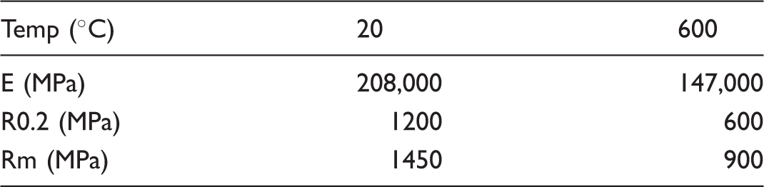
Mechanical properties at different temperatures.
Specimen
All Side Edge Notched Tensile (SENT) specimens are machined by wire cut electro erosion on an AGIECUT 100D wire cut machine (Figure 1). The flat surfaces of the specimens are then ground parallel to the loading axis on an LIP 515 surface grinder. In the last stage, specimens are polished on a metallographic polisher BUEHLER® PHEONIX 4000, to obtain the final thickness with a mirror finish using a 1 mm grit diamond paste.
Specimen geometry.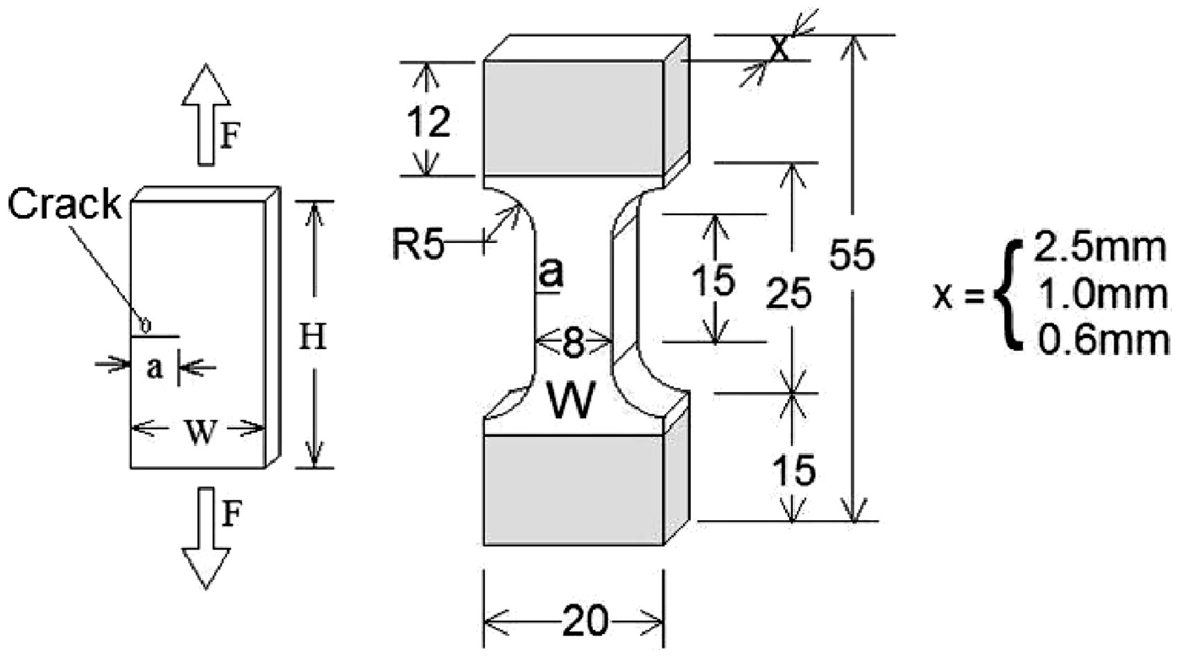
Specimens with two thicknesses (0.60 mm and 2.50 mm) are tested.
Procedure
Fatigue crack growth rate tests
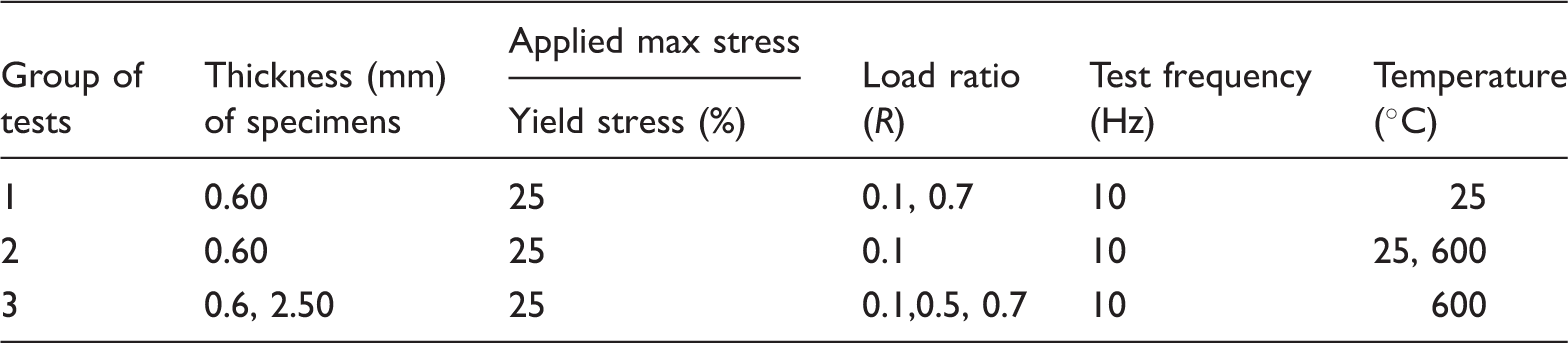
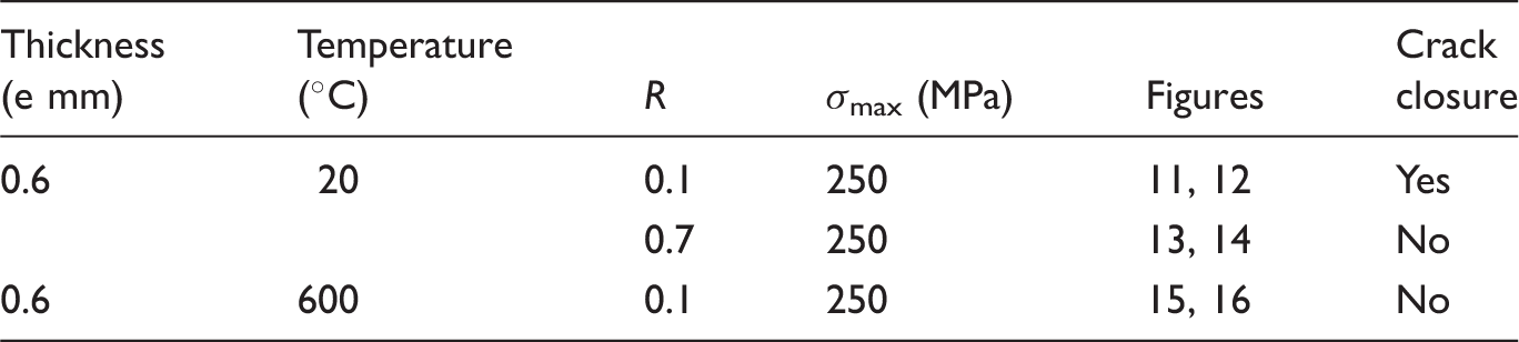
Summary of FCGR tests.
Crack length, COD, and CTOD measurements
The crack length, crack opening displacement (COD), and CTOD measurements are all carried out optically. The crack propagation length is observed optically, in situ with a long distance microscope, without interruptions of the experiment with a Questar Step Zoom 100 (SZM 100), Figure 2(b). It has a maximum optical resolution of 1.1 µm. The field of view, depending on zoom, is between 0.375 and 8.0 mm.
(a) Configuration of the experiment observation microscope, (b) Questar SMZ 100, and (c) CCD camera.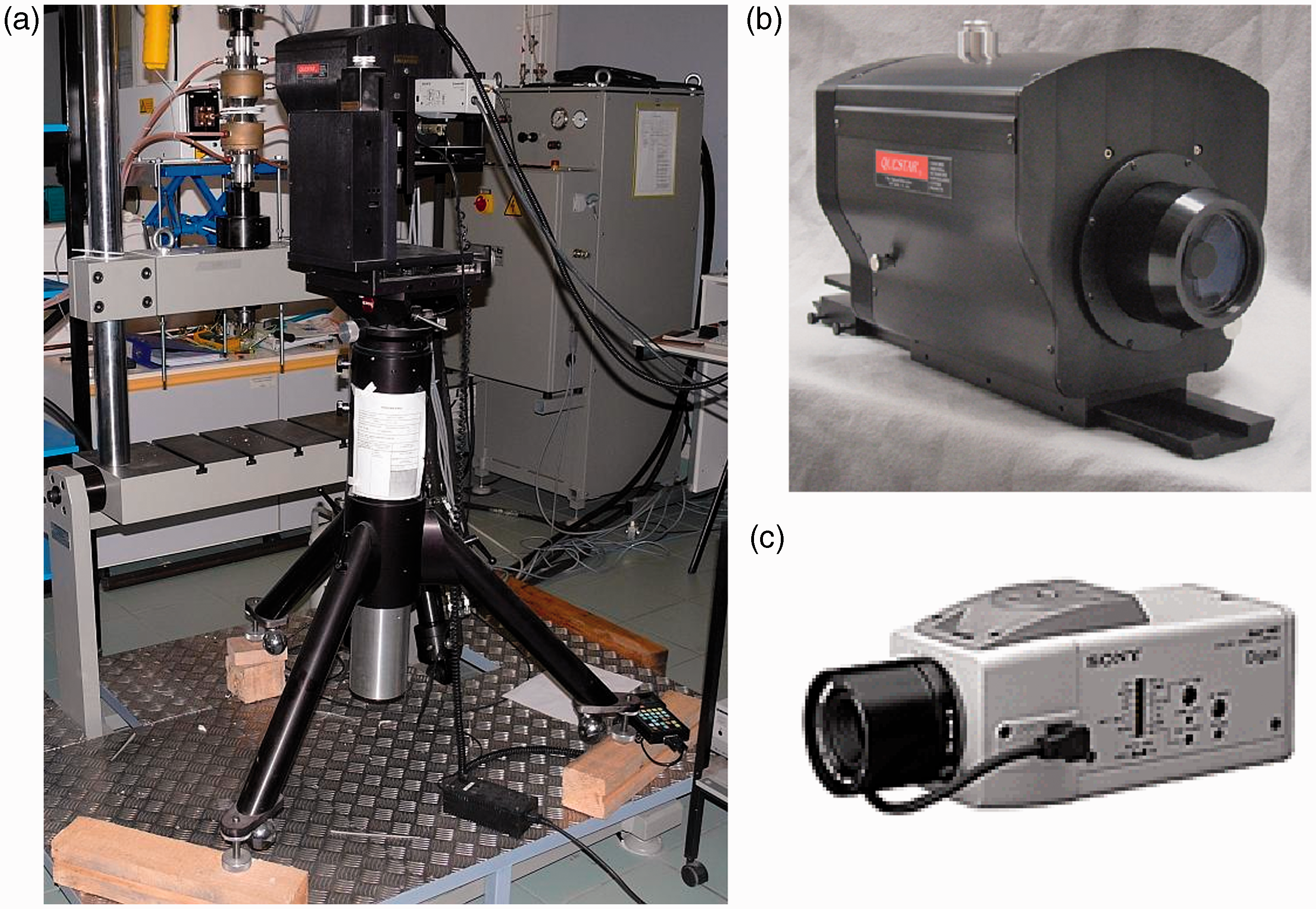
The experimental setup is shown in Figure 2, and is explained in detail by Ktari et al. (2014) as well as a review on image correlation used by other researchers to determine COD, CTOD, and crack length. Figure 3 presents a general overview of the CTOD measurements using image correlation.
Image correlation for crack opening displacement (a) placement of virtual extensometers behind crack tip, (b) reference image (Pmin), and (c) deformed image (Pmax) for correlation.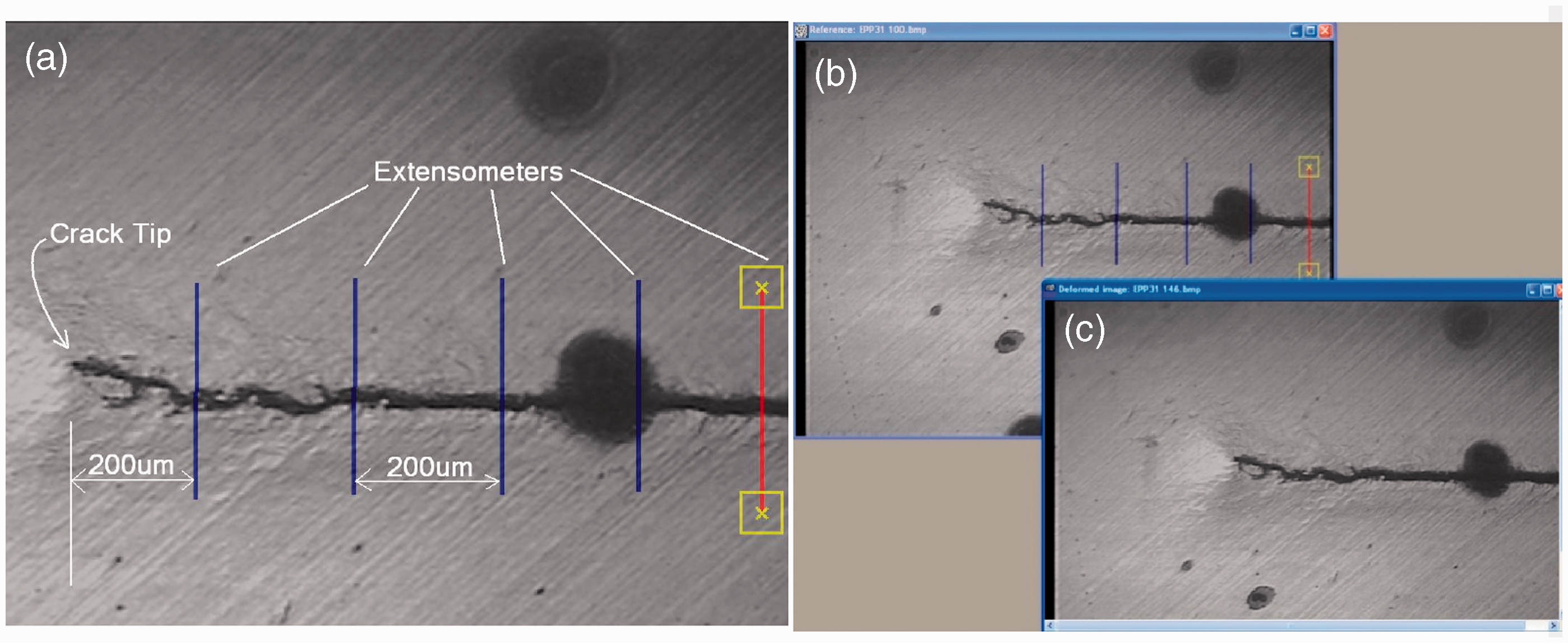
Results
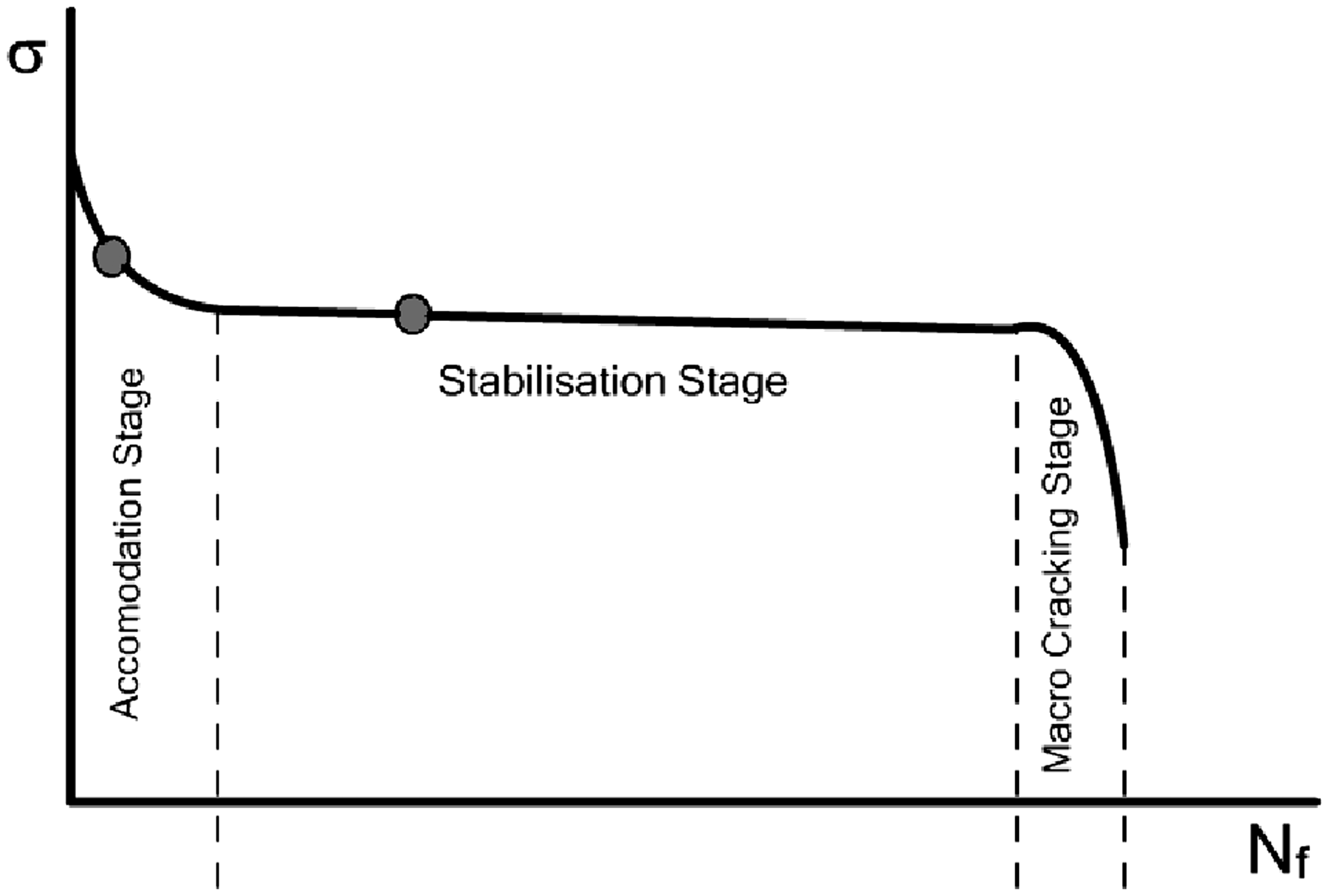
The results of the experiments are grouped according to the method of normalization. All the FCGR data are presented as Paris and Erdogan (1963) curves using the power law

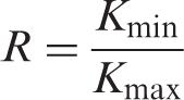
The increase in R ratio is in general considered to increase the crack propagation rate for a given ΔK value. Two methods are generally used to normalize this effect of R ratio on crack propagation curves and are studied in the two following sections.
One method is based on the physical aspects of the effect of R ratio (Elber, 1970). This involves the effect of crack closure which is higher, at lower values of R (typically R = 0.1), and diminishes with increasing value of R. Usually at R = 0.7, the crack closure is considered absent. Due to the closure effects, the crack is shielded from the applied load during a part of the loading cycle even under tensile loads. This shielding causes a reduction in the applied ΔK, which causes an apparent decrease in the crack propagation rate. Use of a ΔKeff parameter (effective SIF range) is found to normalize the results by removing the shielding effects.
The other method is principally empirical and mathematical proposed by Kujawski (2001a). It is considered that the crack propagation rate is no longer a unique function of the SIF range ΔK, but a combined function of the ΔK and the maximum SIF Kmax. The author has explored many possible data normalization techniques (Kujawski, 2001a, 2001b, 2001c; Stoychev and Kujawski, 2005) of which the generalized form seems to be the most adapted to our work (Kujawski, 2001a).
Normalization of R ratio effect on FCGR based on crack closure
The effect of R ratio on the fatigue crack growth rate in the Paris regime is an apparent decrease in the crack propagation rate with a decrease in the R ratio as shown in Figure 4 (Elber, 1970).
Effect of using ΔKeff of Paris curve for R = 0.1 in a 0.6 mm specimen at 25℃.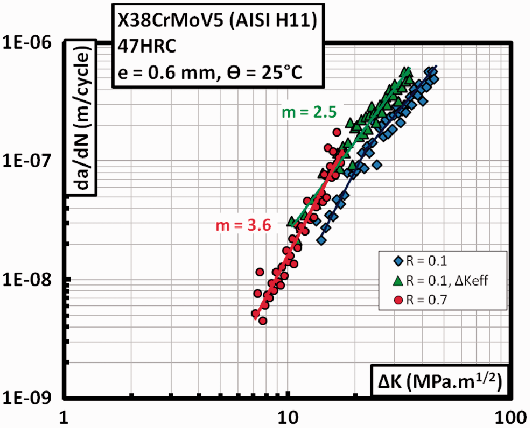
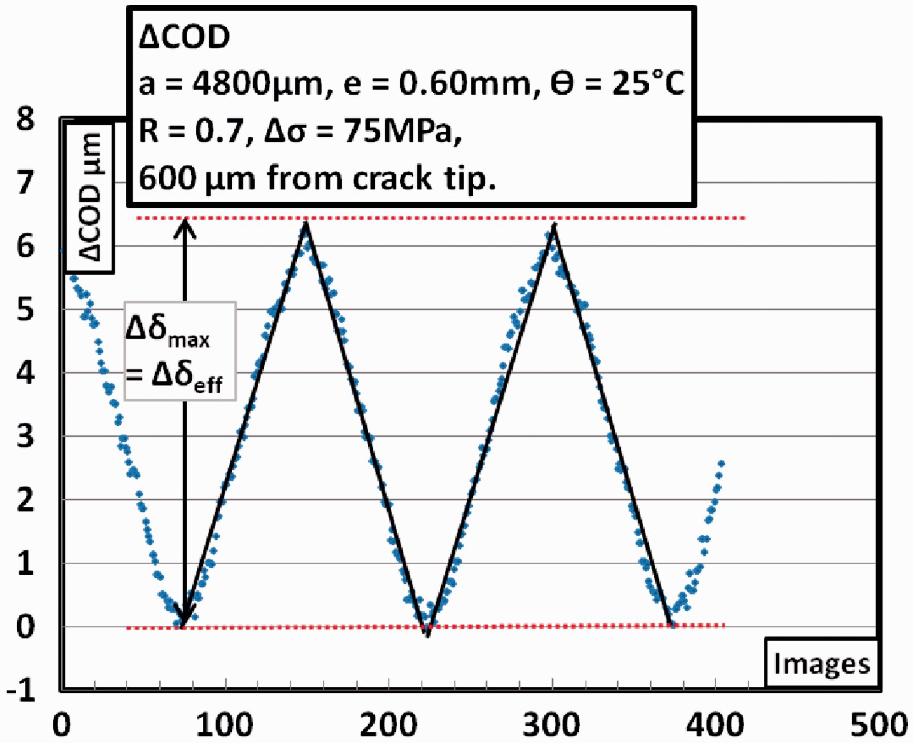
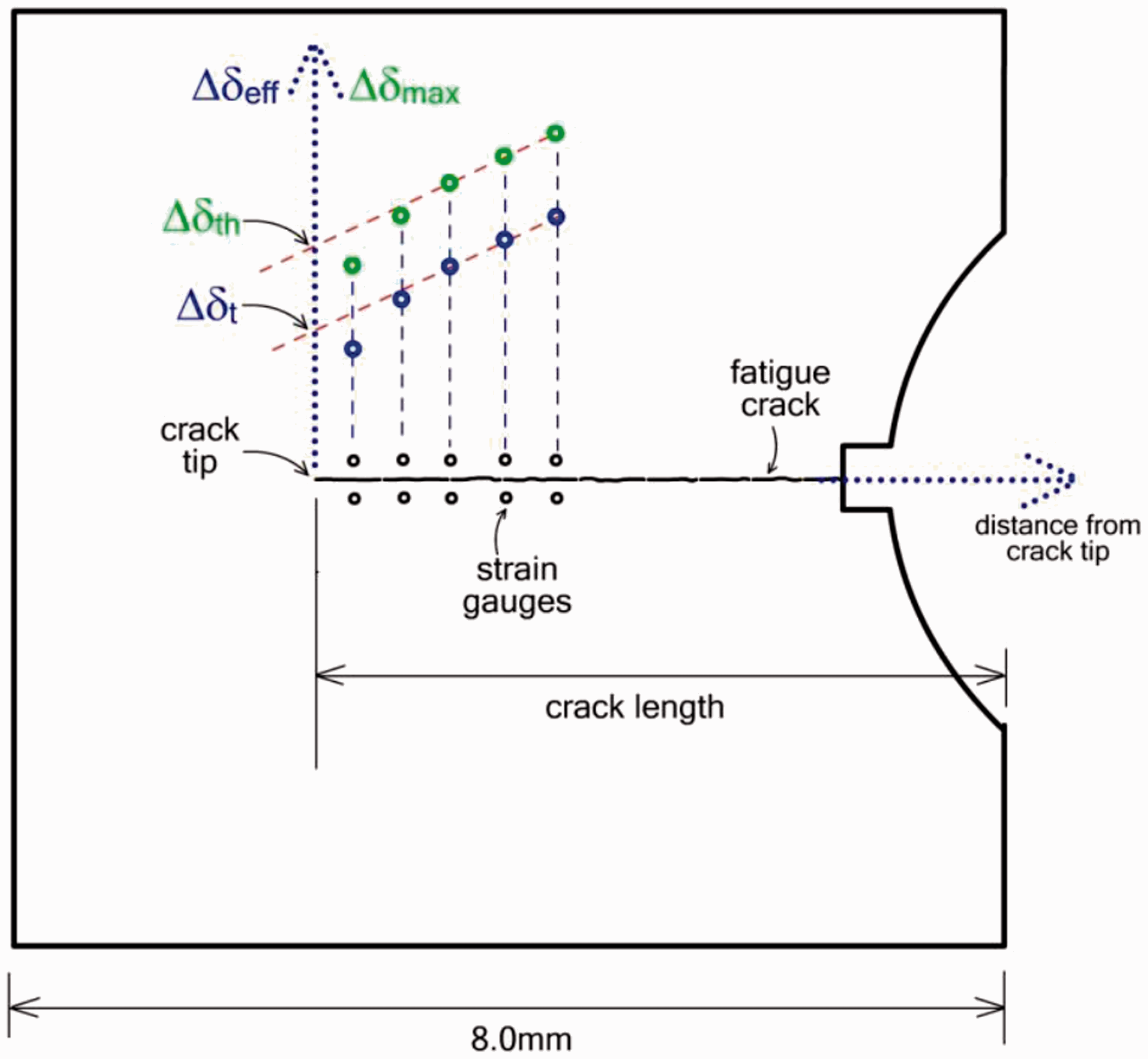
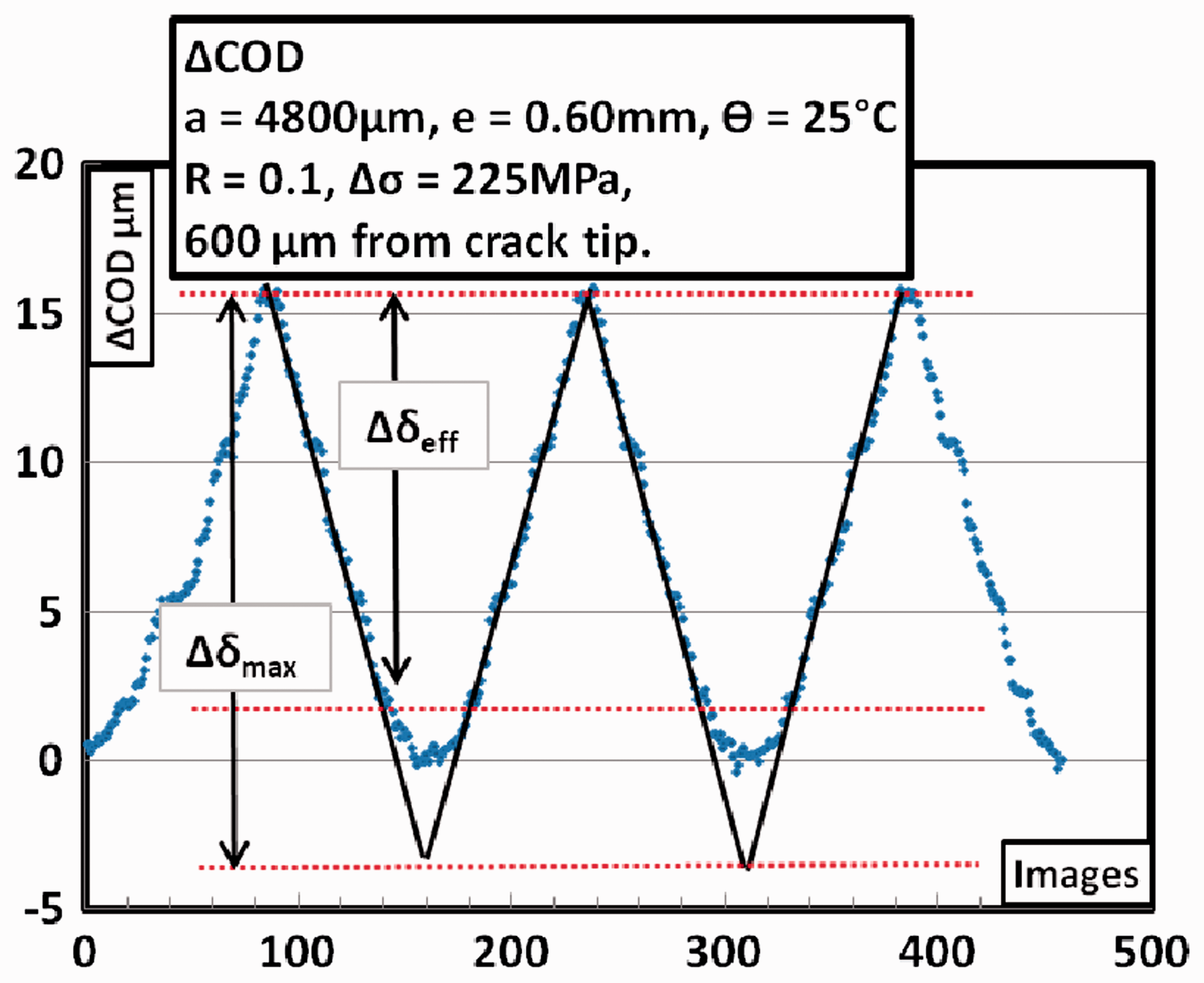
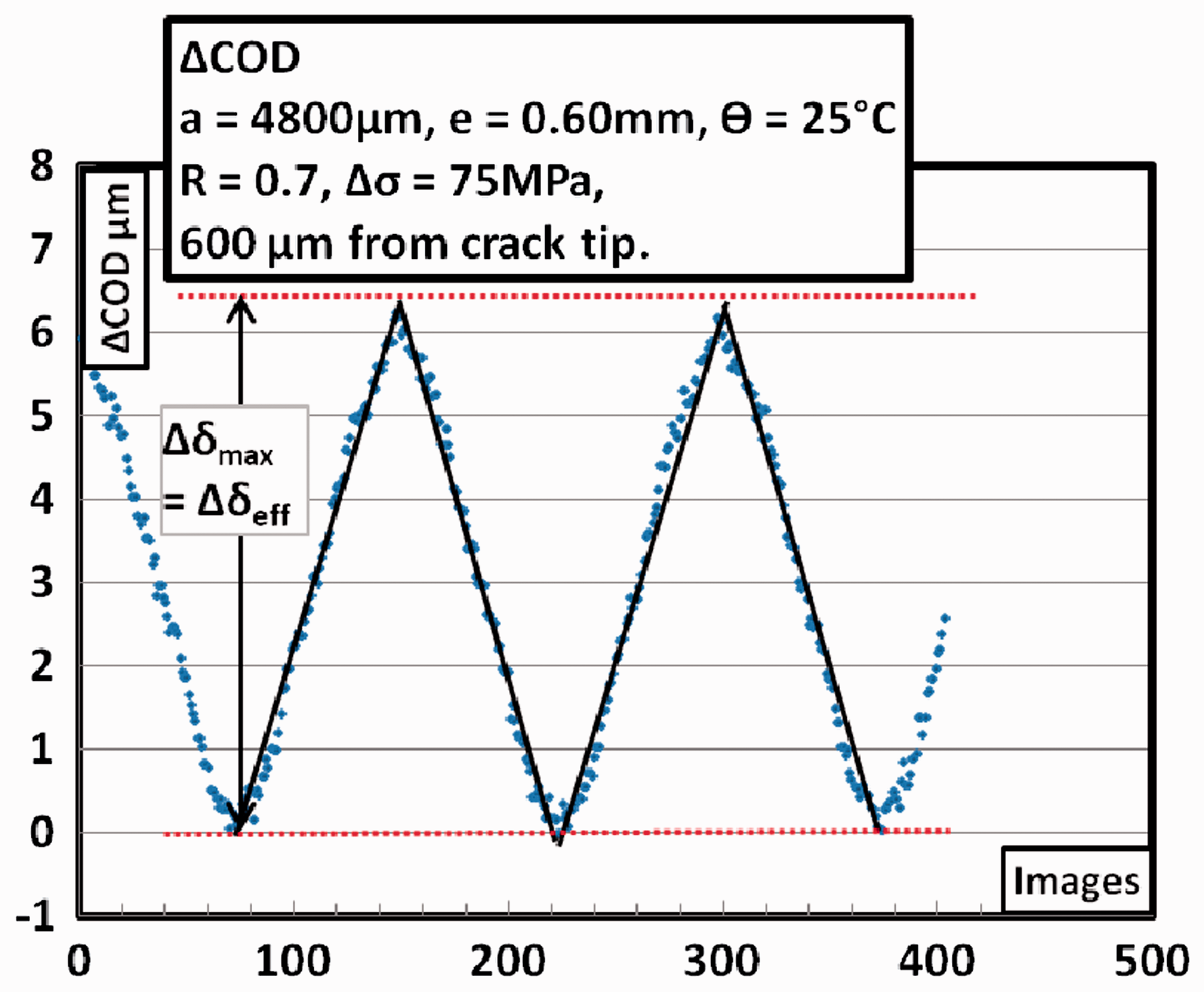
This reduction in the FCGR may be explained by the reduction in the really applied SIF range (ΔK) due to crack closure. To detect this crack closure, a DIC method is used where a virtual extensometer is placed 600 µm behind the crack tip. An unloading curve is plotted between the applied stress and a virtual extensometer COD (Figure 5). Figure 5 shows this for a crack length of 4.8 mm in a specimen of 8.0 mm width. The COD measurements are experimentally carried out between σmax and σmin (so as not to disturb the fatigue experiment). The value of COD at zero load is not accessible, thus the absolute value of δ0 is arbitrary. However, the difference values like Δδeff, Δδmax, etc have physical sense and represent the real displacement of the virtual extensometer as a response to stress range Relationship between applied stress and crack opening displacement measured by a virtual extensometer.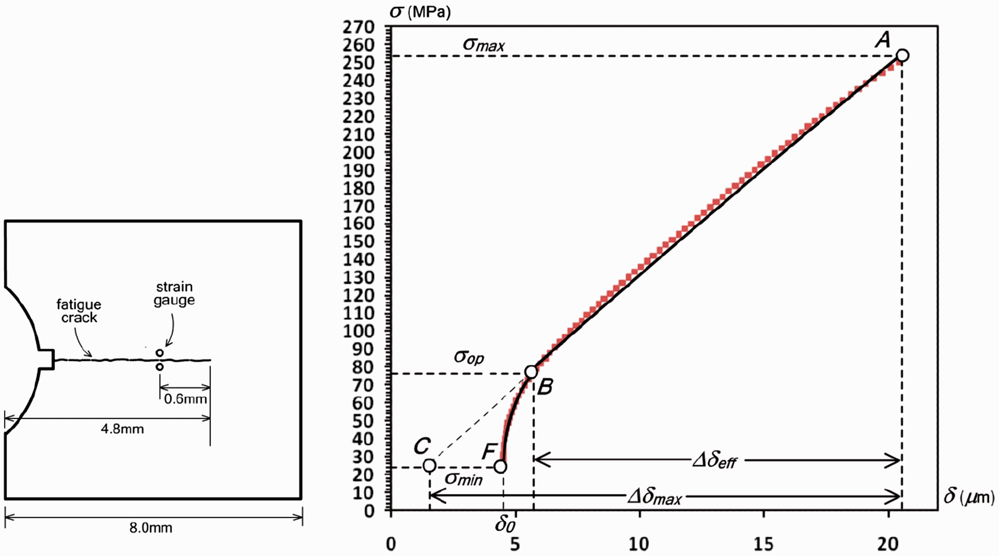
In Figure 5, the region A–B represents the linear variation of the COD with respect to applied stress. From point B, the crack closure begins to appear, right up to point F. The COD corresponding to A–B is given by Δδeff. This is a tension–tension test with R = 0.1, the σmax = 250 MPa, and σmin = 25 MPa. From Figure 5 (Point B), the σop = 75 MPa. From here, the ΔKeff or Reff (Elber, 1970) can be calculated from equations (3) and (4). For this specific case, Reff is found out to be 0.3. In practice, it is easier to present the COD as a function of time or number of images if a triangular load signal is used as shown in Figure 6. In reality, Figure 6 is the same as Figure 5 rotated 90° counterclockwise. The advantage is that the untreated values measured by the machine and the extensometer may be used directly to estimate the Δδeff, δop, and Δδmax. If there was no closure present, then the straight line A–B would continue to point C corresponding to σmin, Figure 5. Thus, the line A–B–C represents the extrapolated crack opening for no closure, the magnitude of which is given by Δδmax.
Variation of δ (COD) as a function of a number of images during fatigue cycles in a specimen of 0.6 mm tested at R = 0.1 showing crack closure.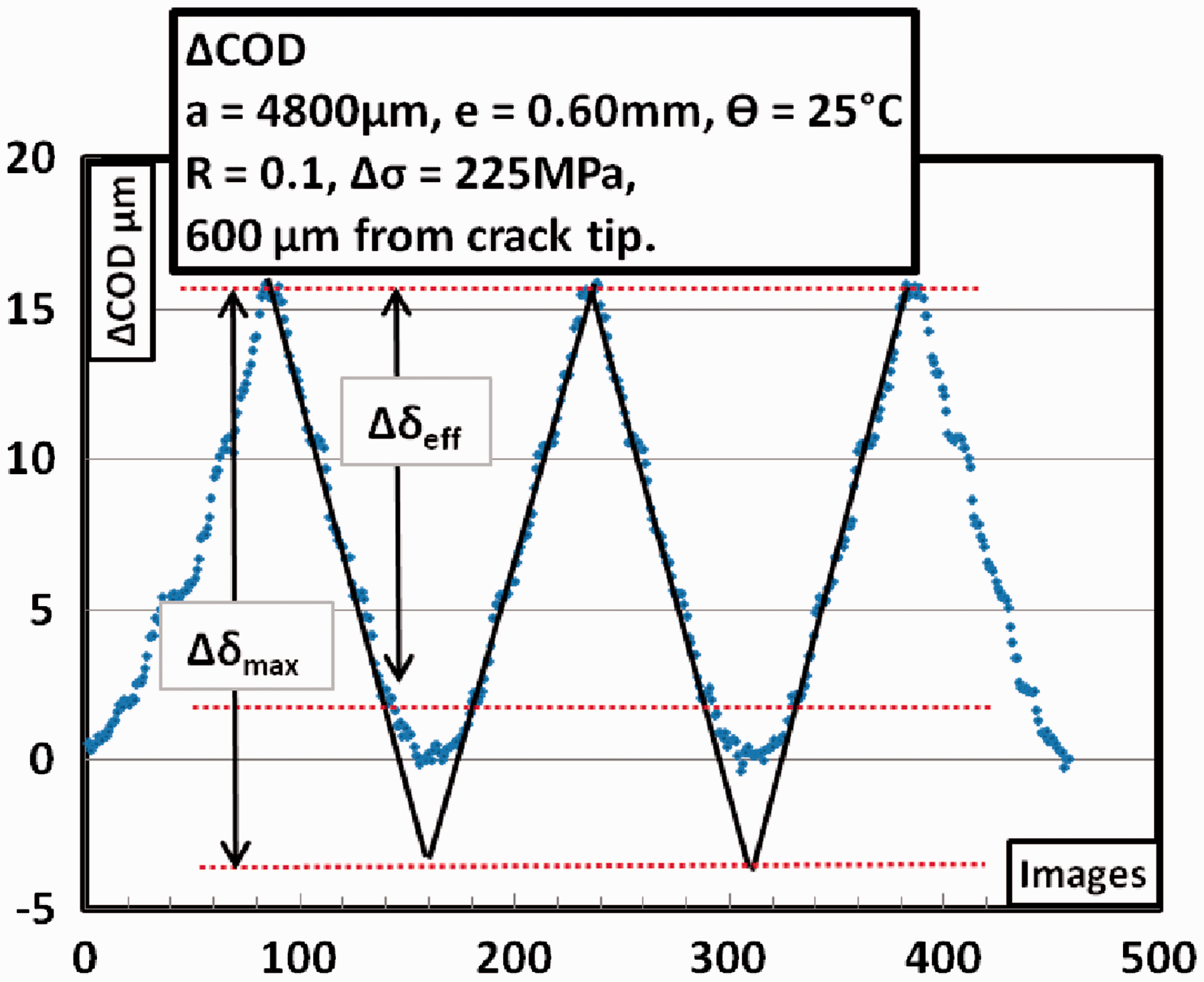
The shielding of the crack tip by closure has a direct effect on the applied SIF range ΔK. The equations (2) and (3) represent the effect of crack closure on the fatigue crack growth


In practice, it is observed that tests carried out at R = 0.1 show the effects of closure (Figure 6), while those carried out at R = 0.7 show no crack closure (Figure 7), in which case Variation of δ (COD) as a function of a number of images during fatigue cycles in a specimen of 0.6 mm tested at R = 0.7 showing no crack closure.
In most of the cases, five virtual extensometers are placed at 200 µm intervals behind the crack tip. However, according to the conditions of the experiment, more extensometers (further from or nearer to crack tip) may be added. The effect of using ΔKeff as a fatigue crack propagation criterion is shown in Figure 4.
ΔKeff correction makes the two curves overlap, however, the slope of the two curves is distinctly different with
This normalization technique only takes into account the crack closure effects. Variation due to any other mechanism cannot be catered for by this method.
Normalization of R ratio effect based on “two parameter crack driving force”
In a propagating fatigue crack, the crack closure phenomenon may be present due to many reasons (Kujawski, 2001a). They include but are not limited to, plasticity, crack wake roughness, oxide formation on crack faces, debris (Suresh, 1998) etc. Any correction for the effects of variation in R based on the crack closure mechanism assumes that as soon as the crack begins to close, it is fully shielded from the applied load. However, this is not always true in reality. In practice, the crack closure does not always account for the difference in crack propagation curves due to variation in R ratio (Kujawski, 2001c).
Problems associated with the crack closure-based models have been reviewed by Kujawski (2001c). To account for the R ratio effects, many different models have been presented based on closure, residual compressive stresses, environmental influence, and the partial crack closure (Kujawski, 2001c; Paris et al., 1999; Suresh, 1998).
The data normalization model presented here removes the need for taking into account the crack closure phenomenon. The model is based on the proposition made by Walker and Lockheed-California Co (1970) reviewed by Kujawski (2001a) according to which there is a close similarity between fatigue life corresponding to crack initiation and that of fatigue crack propagation behavior. He showed that an effective stress 
Equation (5) may be modified and adapted to the fatigue crack growth correlation

As discussed above, the effect of R ratio may be due to many different reasons that are not necessarily dependent on the material properties. Thus, the m in equation (6) may be replaced by α. The α is used to normalize the crack propagation curves at different R values. The equation (6) then takes the form (Kujawski, 2001a)
The damage at the crack tip is due to two simultaneous damage mechanisms based on monotonic damage due to Kmax and cyclic damage due to ΔK. → Existence of tensile stresses in the process zone (Kmax > 0) is a necessary condition for fatigue crack propagation.
There are some interesting properties of α that may be mentioned here. In a case of very brittle material, the value of α → 1, which shows the damage is based on Kmax only. In the case of ductile materials with no effect of R (like under vacuum for some materials) α → 0. For ductile metallic materials, an intermediate value is generally found.
Determining α for fatigue crack
FCG data obtained on two positive R ratios, namely Schematic representation of fatigue crack growth rates at two stress ratios.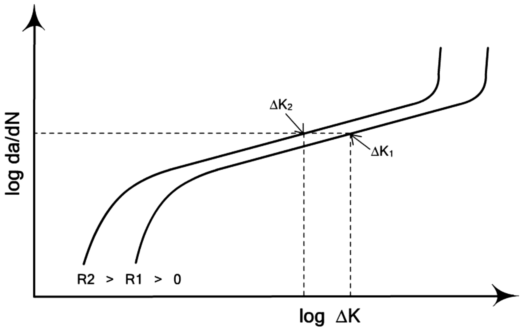
From equation (7), it comes
For normalizing the two curves any da/dN value should lie on the same crack driving force parameter 
Rearranging and taking log on both sides of equation (9) gives
An average αavg may be obtained at different da/dN values along the curve and collapse the FCG data onto a thin band.
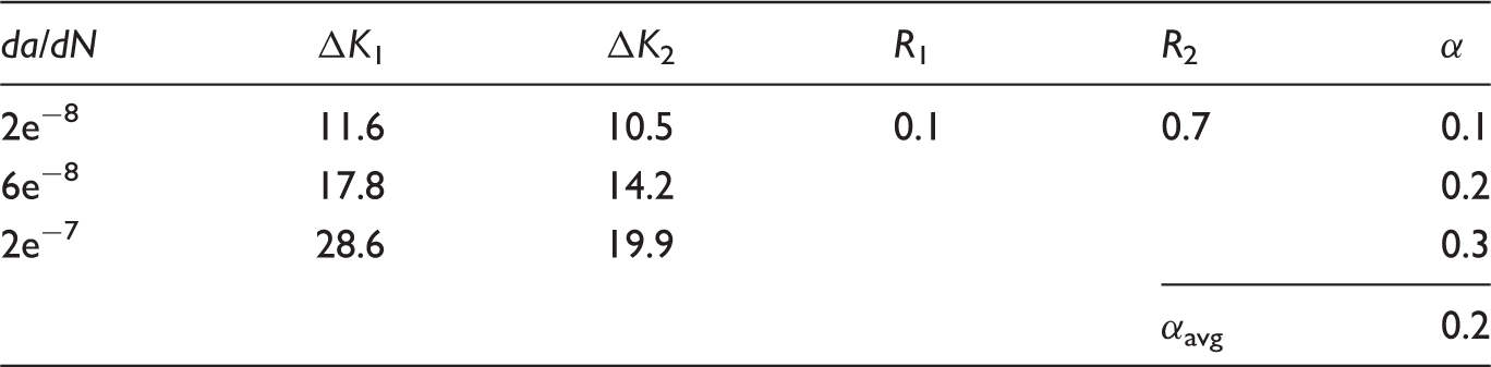
Application on experimental data
This method of fatigue crack growth rate normalization is applied on a specimen of 0.6 mm thickness tested at R = 0.1 and 0.7, Figure 9. The FCGR curve, without normalization is presented in Figure 4. Due to differences in the slope in the R = 0.1 and R = 0.7 Paris curves, a single value for α cannot be determined. Thus, three crack propagation rates of da/dN = 2e−8, 6e−8, and 2e−7 are chosen to determine the value of α. The values of α determined for the three different da/dN values are different. The values of α are summarized in Table 4. An average value of αavg is thus used to normalize the data to a maximum. The two curves overlap for Normalization of fatigue crack growth data for R = 0.1 and R = 0.7, using the Definition of terms used for CTOD criterion Δδeff, Δδmax, Δδ
t
, and Δδth. Summary of α values determined for specimen 0.6 mm tested at R = 0.1 and 0.7.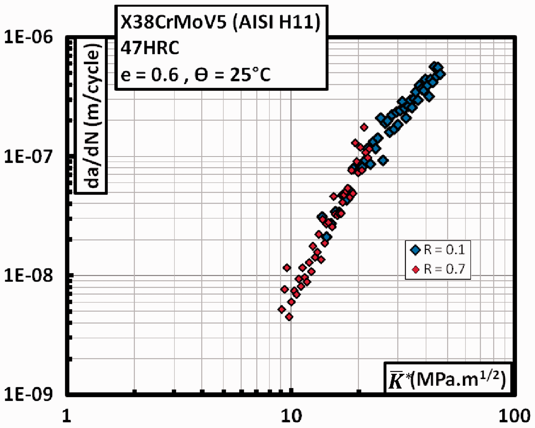
Results are then similar to what was obtained after crack closure correction, with a fair amount of data normalization achieved.
Normalization of FCGR data based on CTOD and the cyclic J-Integral
Theoretical basis of the CTOD and cyclic J-Integral for FCGR application
The two parameters presented previously are based on the LEFM SIF range ΔK with modifications according to the conditions of FCGR. The principal condition that has to be met is the SSY at the crack tip. Under certain conditions (like high temperature), the SSY conditions no longer exist and there is large-scale plasticity at the crack tip called the Large Scale Yielding (LSY) condition. Under such conditions, the ΔK criterion loses its physical meaning. The fatigue crack growth thus needs to be characterized using the EPFM criterion. Two methods are more often used for the EPFM criterion.
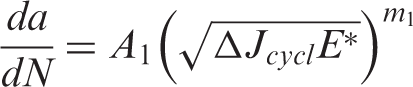
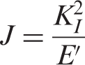
The first is the J-integral of Rice (1968). It is mainly a monotonic parameter that was proposed for FCGR by Dowling and Begley (1976) and Dowling (1976) by giving it a cyclic J-integral definition. Chow and Lu (1991) extensively reviewed and analyzed the cyclic J-integral ΔJcycl. It has been used directly or in different mathematical forms, mostly to match the dimensions. One such form proposed by Sadanada and Shahinian (1979, 1980) for high-temperature testing of super alloys takes the form
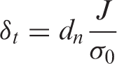
An alternative approach for characterizing fatigue crack growth under elastic–plastic conditions can be formulated in terms of COD. In that case, fatigue crack propagation rates are expressed as function of CTOD range ΔCTOD (or Δδ t ). Using CTOD range as crack driving force has been proposed for instance by Laird and Smith (1962), Pelloux (1970), and Neumann (1973), associated to failure mechanism models linked with fatigue striations. This approach is still used nowadays as a basis for fatigue cracking models, Hamam (2006), Schweizer et al. (2011), and Wang et al. (2004). The problem to be resolved then consists of determining the ΔCTOD.
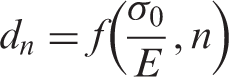
The two methods described above may even be combined, such that the J-integral is determined using the CTOD. The relationship between these two has been principally analyzed by Shih (1981), Hutchinson (1968), Tracey (1976), McClintock (1971), and McMeeking (1977). The complete mathematical treatment is reviewed in previous studies (Ktari et al., 2014; Shah, 2010) and here are presented only the final results of the mathematical treatments. The CTOD or δ
t
is related to the J-integral as
The equations presented above are mainly used for monotonic loading in a cracked material. The problem of the present paper is a case of FCGR and a cyclic definition of the parameters just defined above needs to be made. Thus an adaptation of the above parameters to their cyclic counterparts is presented here (Shah, 2010)
Ability to calculate crack driving force from Δδ
t
. In fatigue experiments, the loading is cyclic. It is in general preferable not to disturb the loading conditions during the experiment. Thus, the ΔCTOD is determined for the stress range Δσ = σmax − σmin. It is not possible thus to have the CTOD value at unloaded specimen (σmin = 0). The form of the crack driving force parameter becomes Find a unique law that shows the Δδ
t
to be a function of R. This is necessary to be able to compare results of crack propagation experiments at different R values. Ideally be able to correlate test results of specimens tested at cold and hot temperatures. Data obtained by Δδ
t
should be comparable to some extent with the numerical simulations carried out for these specimens.
Some of the mathematical derivation will be carried out using LEFM assumptions, especially for the effect of R on the crack driving force.
Under linear elastic conditions
The definition of KI dictates that it is linearly proportional to the applied stress, thus from equation (2)

From equation (14)
The expression (16) shows that ΔK depends on the square root of the Δδ
t
. Also if the R is to be taken into account (necessary to present a coherent fatigue crack propagation law)

Inversely, the equation (17) may be used to calculate the SIF range from ΔCTOD denoted by ΔK
δ
The interest in calculating expression (18) is that if LEFM conditions prevail,
Now in cases where the plasticity cannot be ignored, 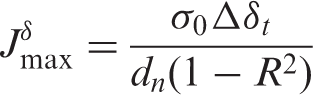

The
For the purposes of fatigue propagation, the ΔJcycl may be replaced by the 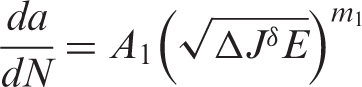
The
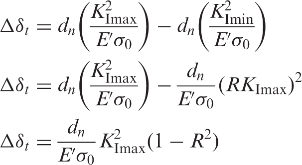
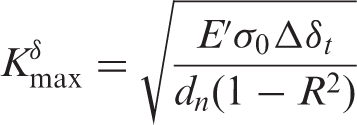
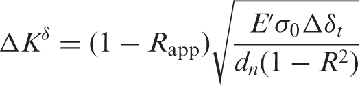
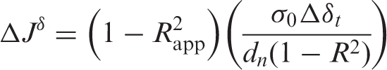
The specimens showing crack closure have different values for Δδt or Δδth. Both of them were tested to find the FCGR criterion that gives the best data normalization. It is observed practically that the Δδth gives better data normalization for FCGR curves at different values of R. An added advantage of using Δδth is the simplicity in its use and calculations, and an R independent criterion may be defined. Equation (22) thus will be modified to
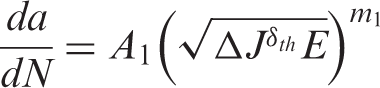
In addition to the criterion in equation (23), the FCGR curves may be obtained by using the 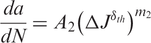
Determination of ΔCTOD (Δδt) under different conditions of R and temperature
The CTOD is measured using the five virtual extensometers technique as shown in Figure 3. The reading of these extensometers ΔCOD is then extrapolated to the crack tip to get a ΔCTOD value. Figure 10 shows this scheme. Some of the terms used in these measurements are defined as below:
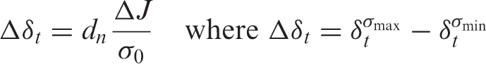
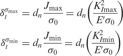
Δδt or crack tip opening displacement (ΔCTOD) is calculated from Δδeff defined in Figure 5.
Δδth is calculated from Δδmax defined in Figure 10.
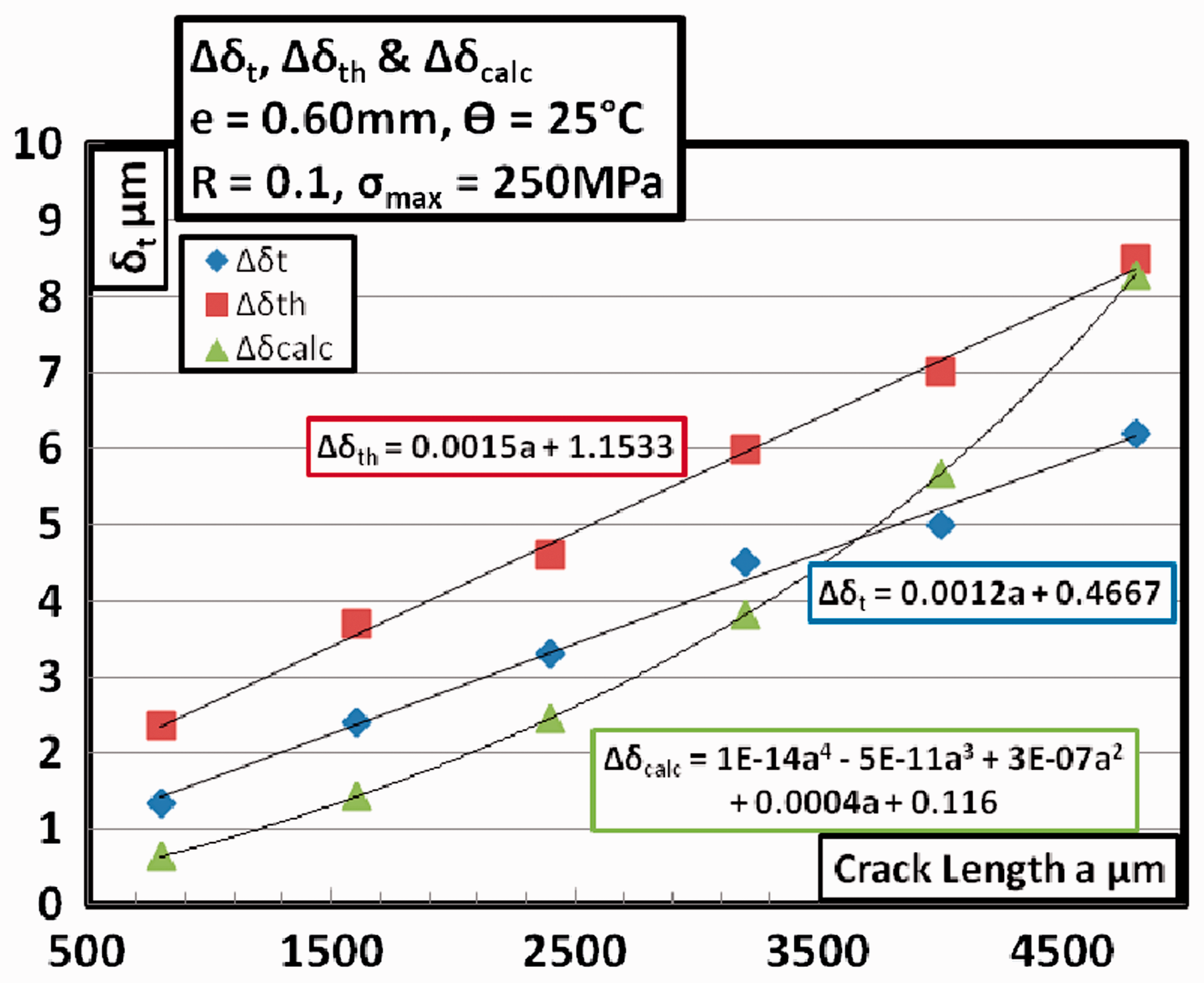
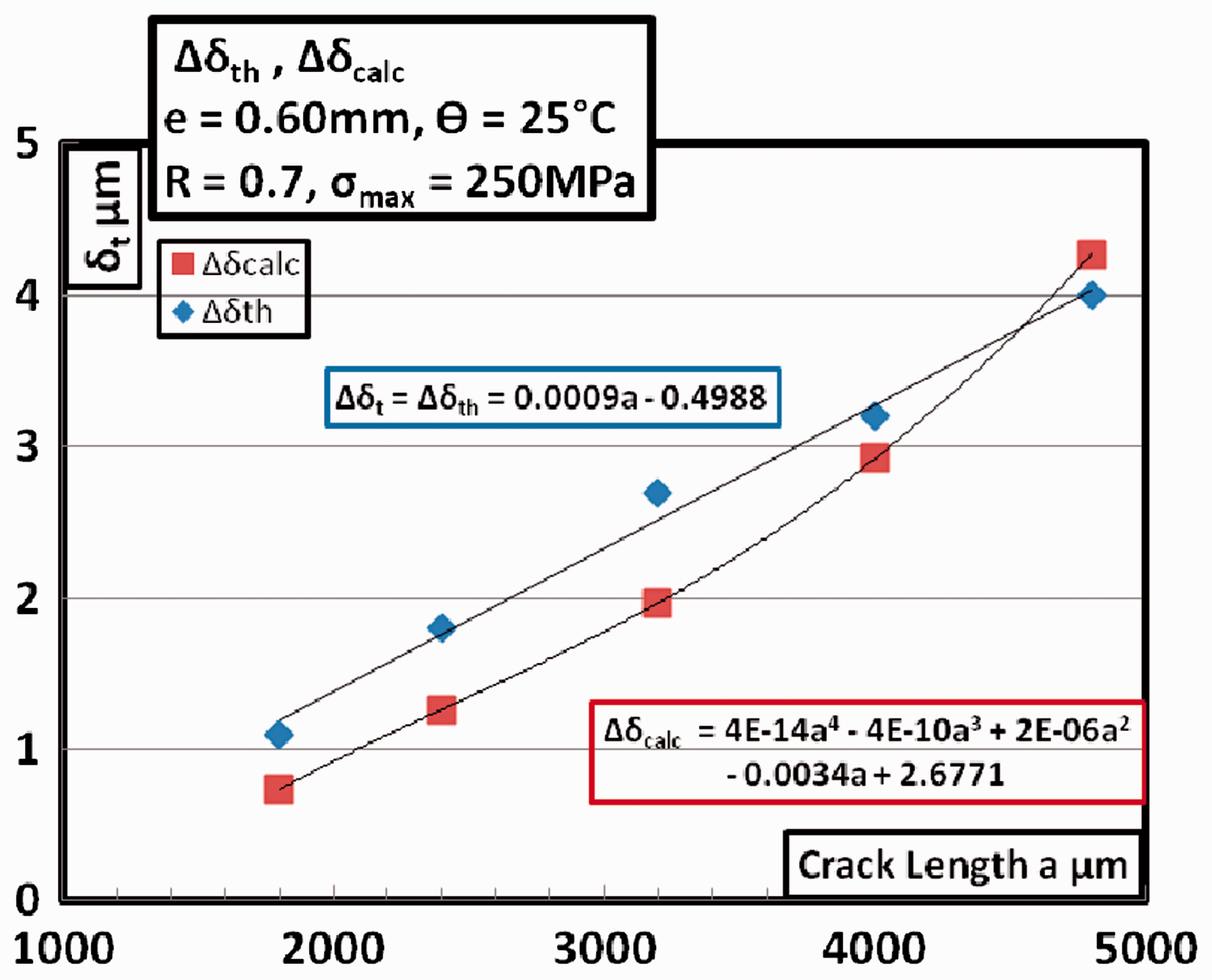
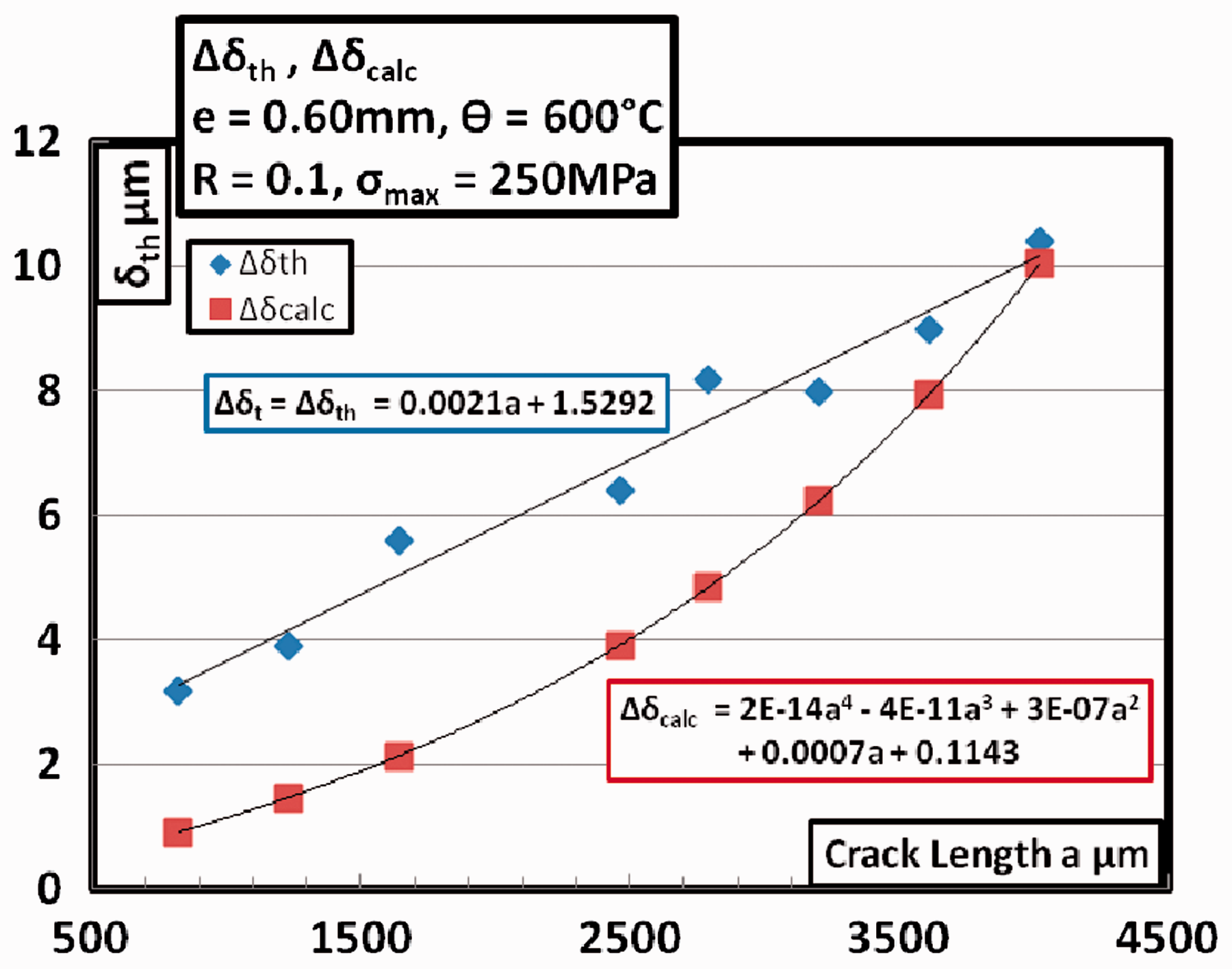
Δδcalc is calculated via J-Integral using equations (14) and (16). The numerically calculated values of J or KI are used directly to calculate this parameter. It is used in validating the hypothesis used in this modeling. This parameter is calculated through J-Integral obtained by numerical simulations done elsewhere (Shah et al., 2012).
An example of Δδ
t
and the Δδth for a crack length of 4.8 mm in a 0.60 mm specimen, tested at R = 0.1 with a maximum stress of 250 MPa, is described in Figure 11. The procedure described here is used for determining Δδ
t
and Δδth values for different crack length extensions in all the cases that have been studied.
Estimation of Δδ
t
and Δδth with the help of Δδeff and Δδmax, respectively. The specimen is of 0.6 mm thickness, tested at R = 0.1 and 25℃.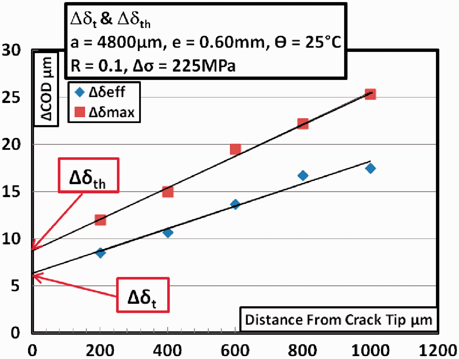
Experimental conditions for the Δδ t and Δδth determination.
The following graphs are present for each experimental condition:
One extensometer reading to determine presence or absence of closure. Evolution of Δδt, Δδth, and Δδcalc and their corresponding mathematical function along the length of the crack during propagation. Crack closure detected by extensometer in a specimen of 0.6 mm tested at R = 0.1 at 25℃. Evolution of Δδ
t
, Δδth, and Δδcalc with increase in crack length R = 0.1 at 25℃. No crack closure in a specimen of 0.6 mm tested at R = 0.7, 25℃. Evolution of Δδ
t
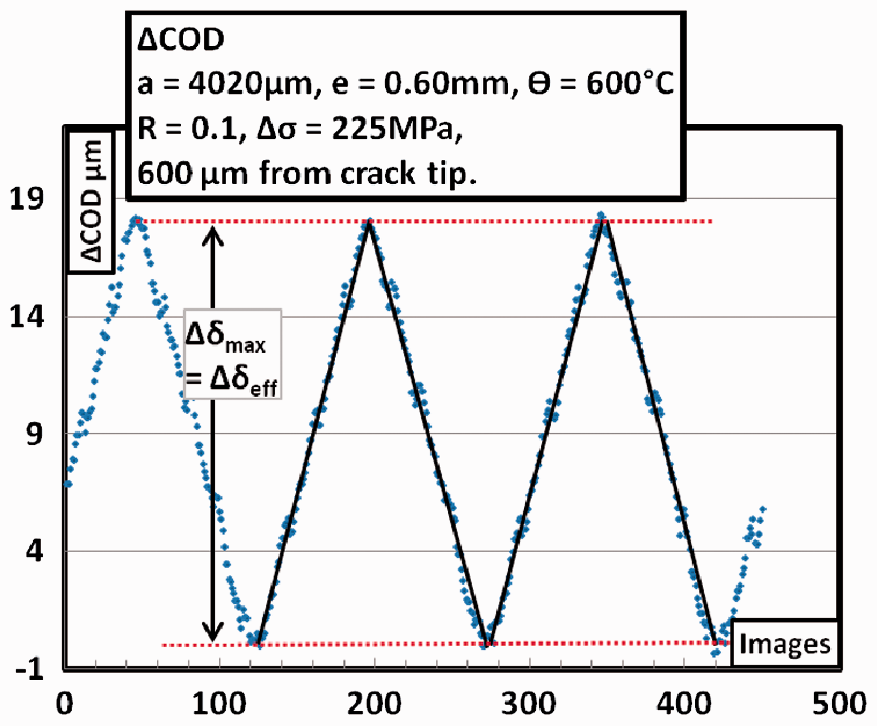
, Δδth, and Δδcalc with increase in crack length R = 0.7 at 25℃. No crack closure in a specimen of 0.6 mm tested at R = 0.1, 600℃. Evolution of Δδ
t
, Δδth, and Δδcalc with increase in crack length R = 0.1 at 600℃.
Figures 12–17 show an interesting trend in the Δδmax and Δδeff. The material shows the presence of crack closure at R = 0.1 at ambient temperature. This is to be expected with the material at these testing conditions. However, of surprise is the fact that no crack closure can be seen for higher temperature propagation even for R = 0.1. The lack of crack closure can be explained by the drop in the Young’s modulus at higher temperature and the effect of creep at higher temperatures demonstrated by the authors (Shah, 2010). It is shown that roughness-induced crack closure due to crack face mismatch exists at low temperatures. At high temperatures, two mechanisms work simultaneously to reduce this effect. First the reduction in Young’s modulus causes the crack to remain more open at σmin. This reduces the possibility of roughness-induced crack closure. The other mechanism is the presence of creep at the crack tip. This has also been demonstrated (Shah, 2010). The presence of creep at every cycle might cause the crack faces to separate as well.
Use of ΔCTOD (Δδt) and
for FCGR data normalization under different conditions
Effect of R at room temperature and 600℃
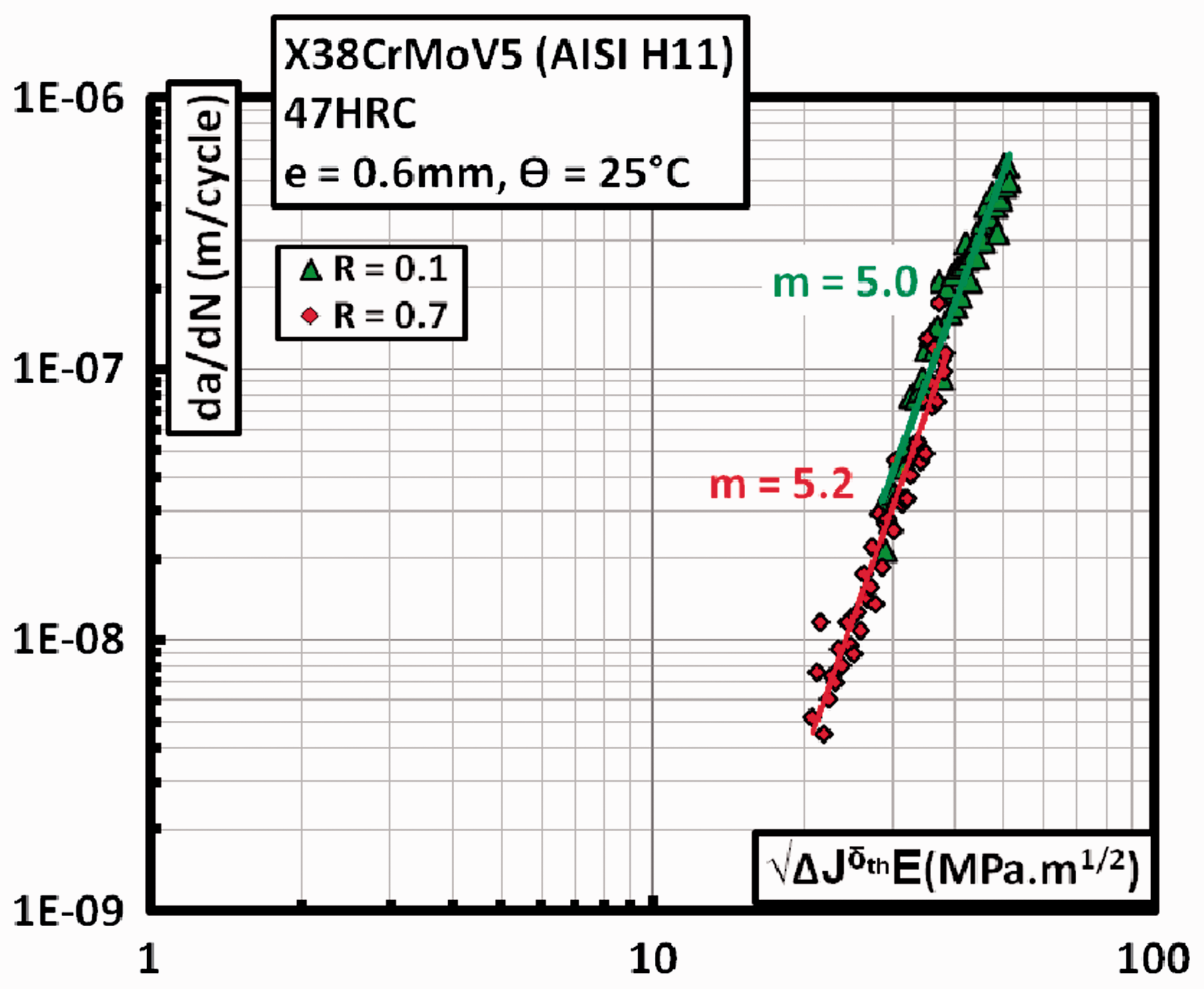
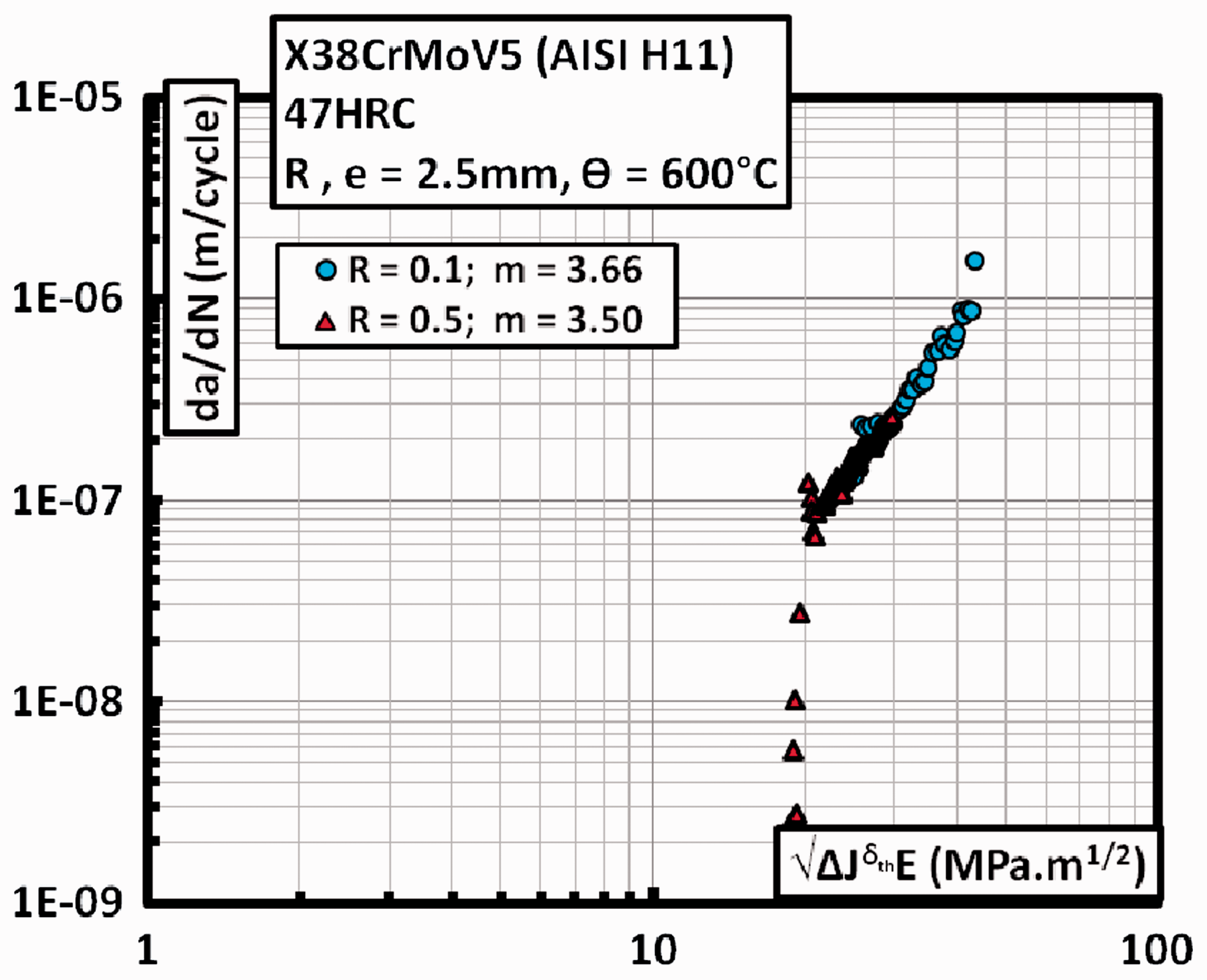
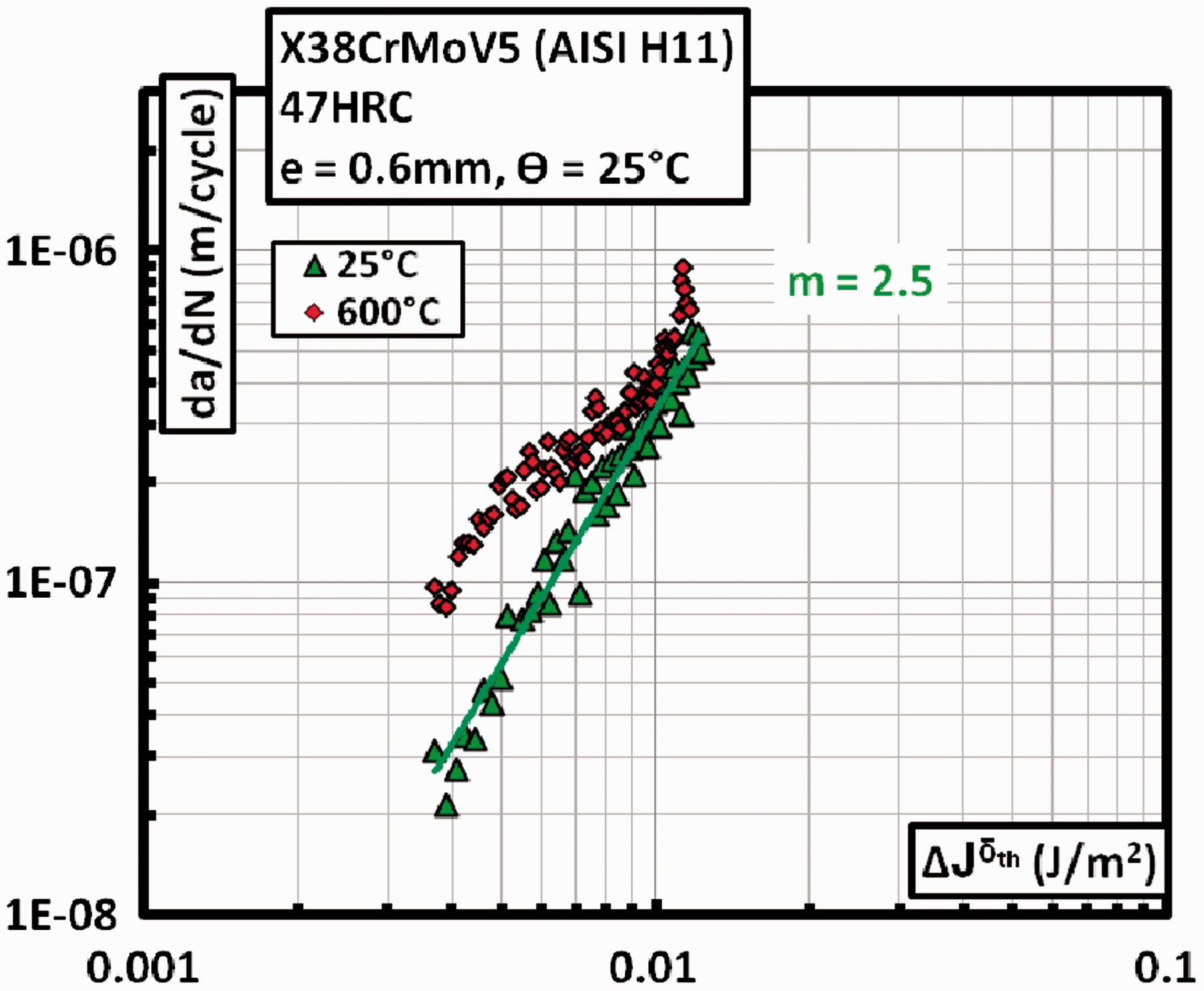
Considering Figure 4, the effect of increase in R ratio was manifested as an increase in FCGR. The use of Δδth directly as a crack-driving force parameter has the advantage of data normalization without any mathematical manipulation as shown in the curve in Figure 18.
Normalization of R effect on FCGR using the ΔCTOD criterion.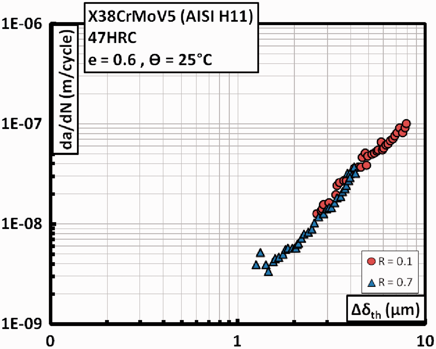
The evolution of Evolution of 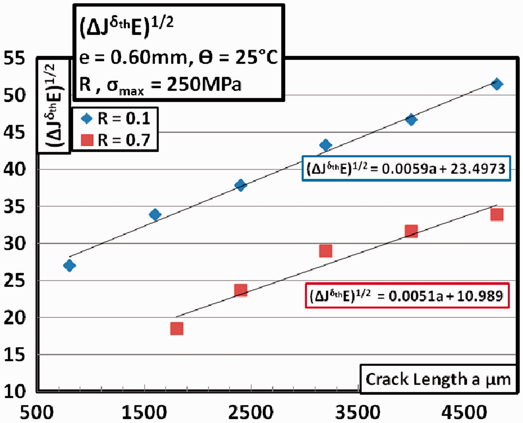
The FCGR curves based on this criterion are plotted in Figures 20 and 22 showing complete data normalization. Also the effect of multiple slopes is seen while using ΔK (Figure 6) has completely disappeared for the specimen tested at R = 0.1 at room temperature.
Effect of R ratio on fatigue crack propagation at 600℃ Effect of R ratio on fatigue crack propagation at 600℃ 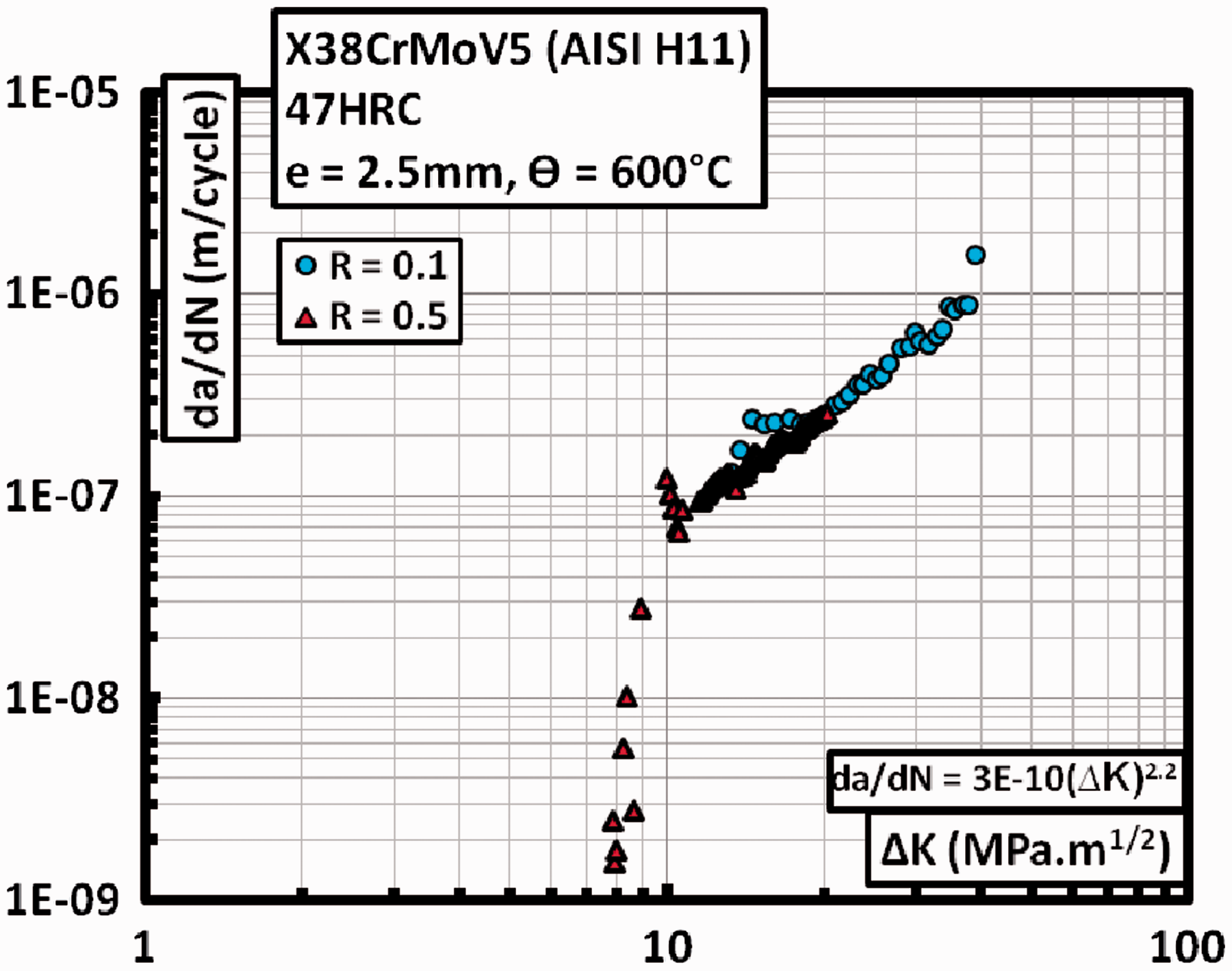
Since the Young’s modulus is the same for the two specimens, the FCGR curves as a function of the crack driving force parameter
The same result can be seen for specimens tested at 600℃ at different R ratios of 0.1 and 0.5. The test had showed no effect of R ratio at 600℃ as explained in Determination of ΔCTOD (Δδt) under different conditions of R and temperature section. The results below show the same trend whether ΔK or
The direct use of ΔCTOD would give the same result as per Figure 22 because all the material properties remain the same, and only units of the X axis will shift.
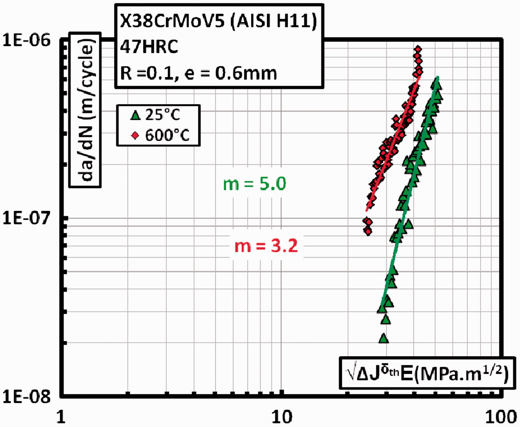
Normalization of FCGR data at room temperature and 600℃
The use of the Δδt or Δδth has the advantage of reflecting any changes in the material properties, since they are measured directly on the specimen being tested. The Evolution of 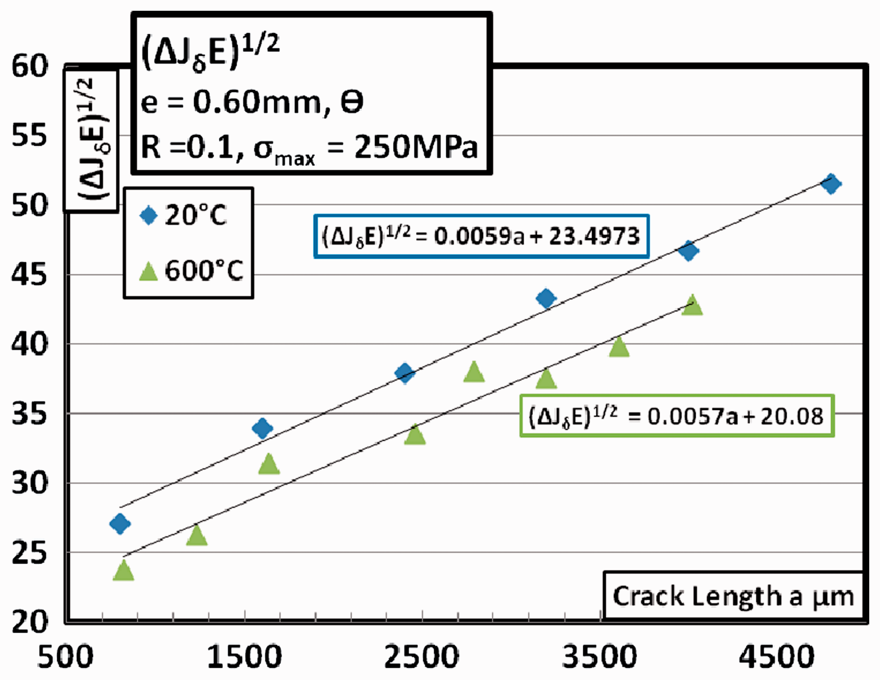
Figures 24–26 show the FCGR as a function of the three parameters Δδth, Δδth as a FCGR parameter at R = 0.1 in a 0.6 mm specimen at 25℃ and 600℃.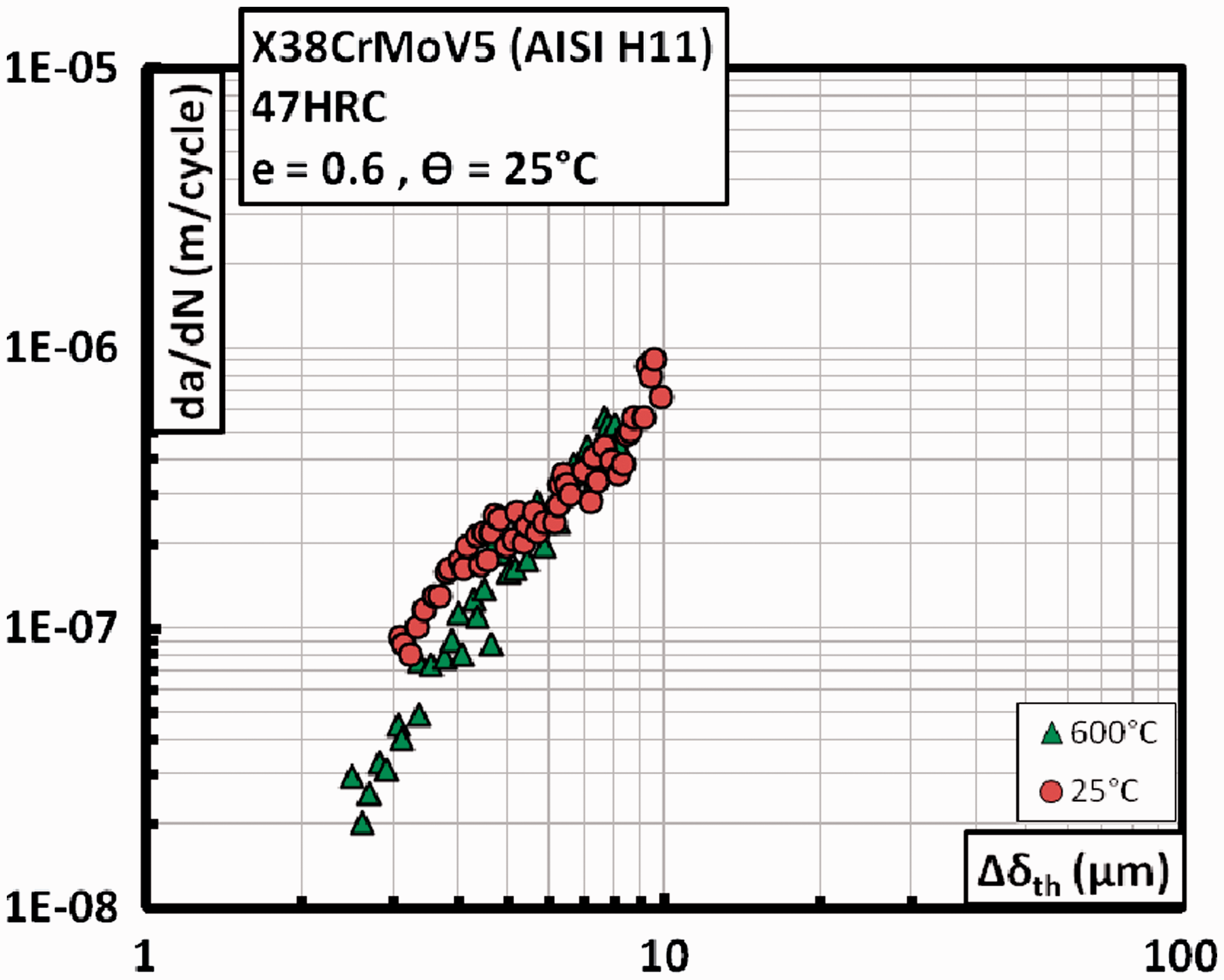
Critical analysis of the crack driving force models
All the crack driving force models presented previously may have some limitations. The limitations may be related but not limited to
→ The physical phenomena associated with the fatigue crack driving force → Mathematical justifications of the model → Assumptions or hypotheses made in the definition of the crack driving force parameter → Material properties → Utilization of monotonic damage criteria on cyclic loading
Normalization of R ratio by:
This model uses an empirical mathematical adjustment to normalize the FCGR data. Its physical interpretation is somewhat vague. The model assumes that the fatigue damage is a function of ΔK and Kmax. It however presents no real physical proof to this effect. The fact that the FCGR may be a function of the average SIF Kav is also a possibility, not explicitly defined in the model.
The model presents no real reference curve to which the data will collapse. FCGR data of different R ratios are displaced by a factor proportional to α toward the left (lower K value) with respect to a simple ΔK-based FCGR curve. The curves at different R ratio will be displaced in the same direction, by different amounts to achieve superposition.
The model may represent false results for cases where there is no effect of R ratio or there is absence of crack closure. For example, α is calculated as a unique value using FCGR data for R = 0.1 and 0.7 in this study. H11 tool steel tested at room temperature shows no crack closure for R ≥ 0.3. This is because at R ≥ 0.3, the σmin is high enough to keep the crack faces separate. Since the closure is due to crack face roughness and mismatch, the faces do not touch at this R value. Thus, all FCGR curves for R ≥ 0.3 will coincide on a single Paris curve calculated on the basis of simple ΔK. The correction applied by
J-Integral as a damage parameter
The J-integral Rice (1968) on its own has been developed by assuming a nonlinear elastic material. This causes problems because the unloading of this material has to follow the same path as the loading curve. This is not the case because real metallic materials most often show an elastic–plastic behavior, which while unloading simply follows a linear elastic path. Thus, the definition of the cyclic J-integral presents difficulties and is ambiguous. Chow and Lu (1991) have performed a detailed critical analysis of the cyclic J-integral, the use of which, for fatigue, was first proposed by Dowling (1976). The main problem with the definition of the cyclic J-Integral arises when it is compared to the SIF for SSY conditions. For a specific case of fatigue crack propagation, when a material is cycled between σmax and σmin, the SIF range ΔK is given by

The cyclic J-Integral may be presented as the difference of the monotonic J value at σmax and σmin, which we will call Jmax and Jmin, respectively
However, for SSY conditions by Suresh (1998):
Now the cyclic J-Integral may be defined as either

Or,


This difference in the definition of
In this study, the SIF range has been calculated by calculating the Kmax from Jmax using
The same problem arises when using the ΔCTOD criterion as a parameter linearly proportional to loading. Since
Cyclic J-Integral calculated using
as a damage parameter
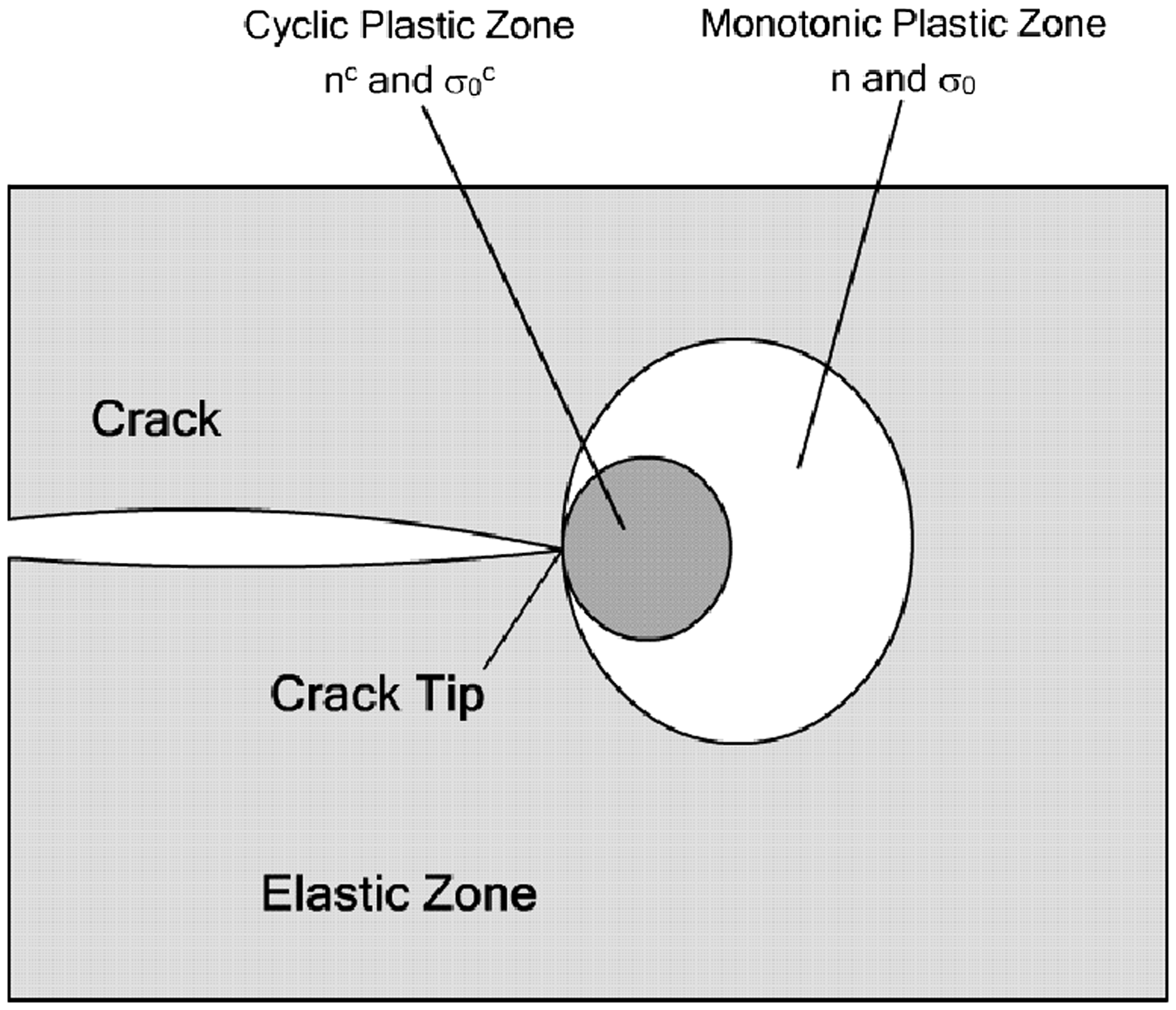
Material properties
The basic expression
The other issue is that the material used for the study follows a power law-hardening behavior under monotonic tensile stress, and thus can be easily characterized by
Cyclic softening under imposed deformation isothermal LCF testing. The cyclic plastic zone may lie on any part of the curve (gray spots). Variation of material constants with respect to the monotonic and cyclic plastic zone at the crack tip.
Large-scale yielding in front of crack tip
The expression of J-Integral has been found to be valid and path independent in large-scale yielding conditions for the unique case of Dugdale type thin strip yielding (Chell and Heald, 1975; Chow and Lu, 1991; Rice, 1975) even though the nonlinear elastic material assumption is invalidated. However this path independence has been studied extensively by Shih (1981), McMeeking and Parks (1979), Shih et al. (1979), Shih and German (1981) on center-cracked panels (CCPs), edge-cracked panels (ECPs), and cracked bend bars (CBBs). They have determined that the region dominated by the singularity fields is dependent on specimen geometry and material-hardening behavior. They have concluded that the size of Hutchinson-Rice-Rosengren (HRR) Singularity Field is greater for the CBB than for CCP. The dominating region for ECP (used in this study) lies in between the two. They suggest that the relationship between J and δ t as expressed by equation (14) will continue to hold for hardening materials where the uncracked ligament (under generalized plasticity) is subjected primarily to bending and may not be valid for ligaments under primarily tensile loading.
Shih (1985) has also presented the analysis of fully plastic edge cracked specimens where it is suggested that a deep crack in an edge-cracked plate may give an important HRR-dominant zone due to an important component of bending stresses. However, the fact that the specimen in our experiments is fixed grip type may increase the tensile component of the crack tip stresses and thus reduces the HRR-dominant field.
Care must thus be taken when using the J and δ t relations (equation (14)) in fatigue crack propagation experiments in SENT specimens especially at elevated temperatures. At elevated temperatures, the hardening exponent becomes low and there is a larger possibility of a generalized plastic deformation.
Conclusion
In this research, different models to analyze fatigue crack propagation in hot work martensitic tool steel X38CrMoV5 (AISI H11) are investigated. Most of the models are developed to be able to normalize the FCGR curve obtained at different experimental conditions. Of interest are the variations in the R ratio and the effects of temperature.
A model for the normalization of the effects of the R is studied. The model is mostly empirical in nature based on mathematical normalization of FCGR curves by considering the fatigue crack propagation as a function of a two-parameter law based on Kmax and K.
Detailed methodology is presented to use DIC for measuring crack closure effects and the ΔCTOD (Δδ t ). The values for these parameters under different conditions are determined. It is seen that there is no crack closure even for R = 0.1 at elevated temperature.
The effect of crack closure is taken into consideration in a second model, using effective SIF range (ΔKeff) determined thanks to DIC measurements. The effect of R ratio on FCGR curves at room temperature is thus normalized.
The use of the J-Integral (Rice and Rosengren, 1968) for fatigue crack propagation is also presented. The J-Integral may be determined using measured ΔCTOD (Δδ t ) values by optical observation of the crack faces during fatigue crack propagation experiments. Most of the parameters and the methodology used are discussed. The parameters defined are then used to create the FCGR curves and make comparisons. It is found that the use of ΔCTOD as an FCGR crack driving force parameter is interesting and presents an R independent alternative to the simulated ΔK parameter.
In the last section, a critical analysis of all the proposed models is presented. All the models stated above are based on certain hypotheses and assumptions that may render them inaccurate in certain conditions.