Damage tolerance in parallel systems

Abstract

Damage tolerance is a fundamental prerequisite for the safety and robustness of large complex systems. Here we analyze the response of a system of parallel rods under a damage event. The approach is based on the presence of multiple load paths in a complex structure, that is, various ways to perform a task. We found that, as much as the complexity increases, the presence of effective ways of carrying the load becomes crucial for the robustness of the structural system under a damage process acting at random on the structure. In addition, the size of the system plays an important role: although tendentially more fragile, large systems are able to redistribute and absorb the effects of damage even with low complexity. The results, here discussed with reference to mechanical systems, can be exported to other disciplines.

Keywords

Damage tolerance complex systems structural engineering parallel systems redundancy

Introduction

Systems working with parallel elements are common in many disciplines. In general, such systems are composed by various entities acting together and at the same time under an external stimulus. Because of the possibility to reassign tasks to single elements, such systems may be considered, in a certain sense, tolerant to damage. On the other hand, systems made of serial elements are not robust: the failure in a single element compromises the whole.

A very intuitive difference between parallel and serial systems is represented by the probability associated with the system failure as the combination of the failure probabilities of the single elements. When considering serial systems, if $P_{f}^{i}$ is the failure probability of the ith element, the probability of failure of the system, $P_{f}^{S}$ , is given by the union of the n single probabilities, that is

P_{f}^{S} = P_{f}^{1} \cup P_{f}^{2} \cup \dots \cup P_{f}^{n} = ⋃_{i = 1}^{n} P_{f}^{i}

(1)

On the contrary, when elements are arranged to work in a parallel configuration, the system failure probability $P_{f}^{S}$ is given by the intersection of the n single probabilities of failure, that is

P_{f}^{S} = P_{f}^{1} \cap P_{f}^{2} \cap \dots \cap P_{f}^{n} = ⋂_{i = 1}^{n} P_{f}^{i}

(2)

It is clear that the extension of the safe domain is much larger in the case of parallel systems, see Figure 1.

Figure 1.

Safe and Unsafe regions are plot describing systems made of elements in parallel and in series. The lines represent the threshold between safety and unsafety, that is, 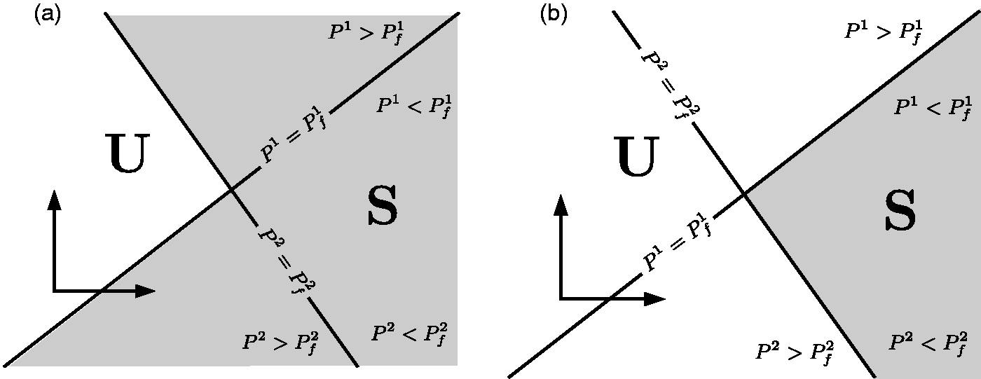$P^{i} = P_{f}^{i}$ . (a) Parallel system. (b) Serial system.

Systems made of elements working in parallel can be found in many disciplines. As a first example, consider the ways an audience is informed about news. The reporter can choose one or more communication media: internet, newspapers, TV program, radio and so forth. In a fictitious world, for preliminary consideration, suppose that the communication has a preferential channel: internet. Other ways are present but not enough used and, thus, developed. What happens if, say, the internet does not work properly, or if some regions are not covered by high-speed internet connections? No information is transmitted and the system fails. On the contrary, if all communication media are constantly used and developed, a local interruption is replaced by other technologies without global communication failure.

Despite the simplicity of the previous example, a similar problem can be easily related to emergency communication in areas where natural hazards are present. In order to present some systems that act with parallel elements, a brief but not exhaustive review is presented in Table 1. In general, following a stimulus, S, the system acts in order to output a response, R. In a mathematical form, what is performed by the system can be described by a function, f, in such a way that

R = f (S)

(3)

Table 1.

Examples of parallel systems in various disciplines.

Stimulus, S	System, f	Response, R
Force	Mechanical stiffness	Displacement (Landau and Lifshitz, 1959)
Emergency	Communication media: internet, newspapers, radio, TV programs	Population's awareness
Body infection	Immune system: surface barriers, inflammation, lymphocytes, leukocytes	Body defense (Parham, 2009)
Moving demand	Routes and means of transport: walk, bicycle, car, coach, train, airplane	Traveling time (Cascetta, 2001)
Energy demand	National and international policies: fossil, nuclear, renewable, global warming, decrease in energy consumptions	Civil and industrial exploitation of energy (Leal Filho and Voudouris, 2013)
End product	Sales techniques: dealer, selling agent, e-commerce, door-to-door	Incomes (Aven and Renn, 2010)
Good demand	Availability, competitors, distribution system	Price to consumer (Gans et al., 2011)
Need of raw materials	Political affairs	Economical and international decisions

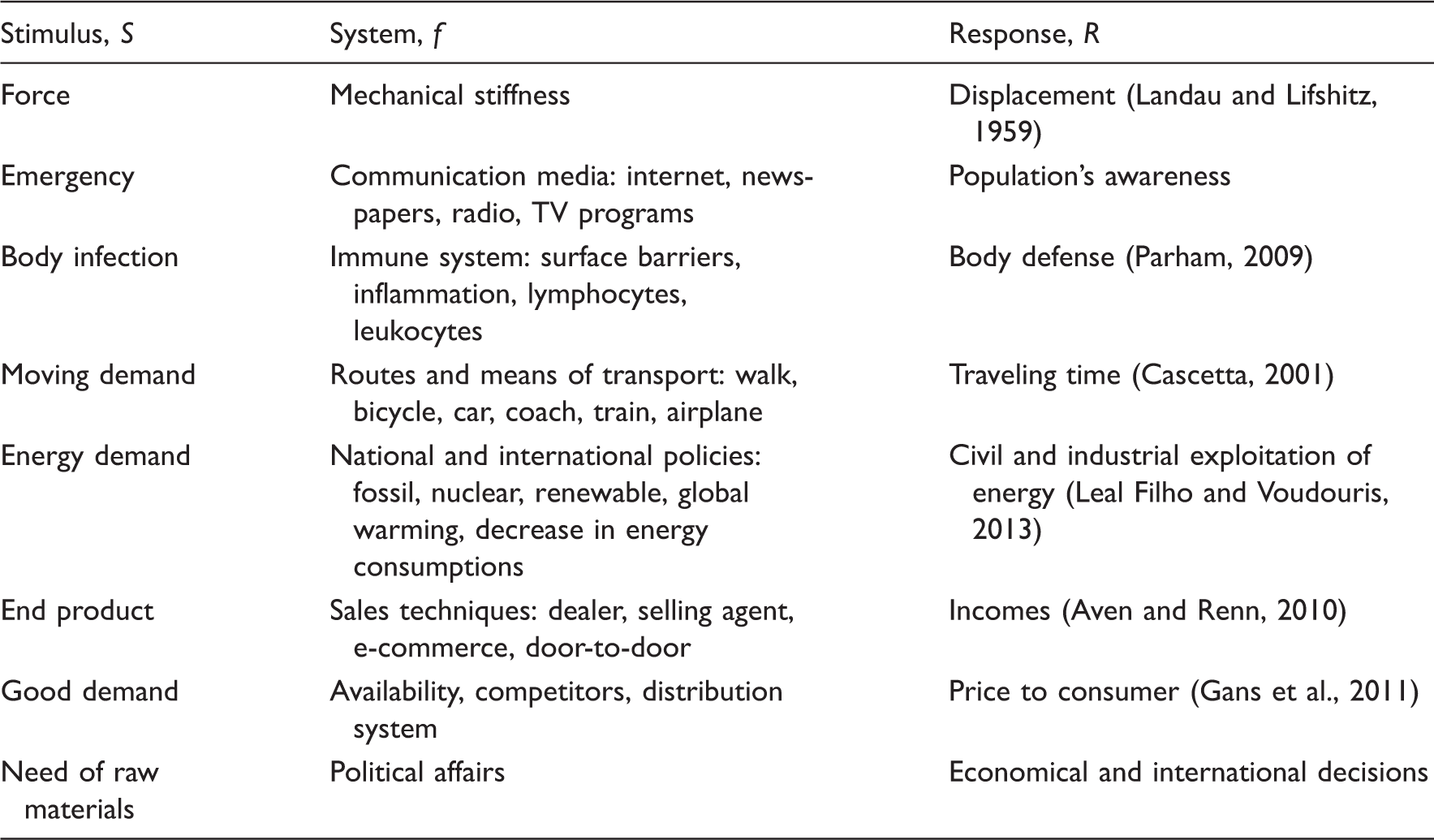
The first line of Table 1 relates to mechanical systems. A spring, if loaded, increases its length. Hooke's law states that the force required to extend or compress the spring is proportional to length increment, or decrement, with a constant factor, called mechanical stiffness. Replicating the springs, a mechanical system is created.

The response of a mechanical system under a damage can be studied. The concept of damage tolerance in large systems has been highlighted by Albert et al. (2000). They found that many complex systems display a surprising degree of tolerance against errors. Despite their attention being on network systems, they found that error tolerance is a property that is not shared by all redundant systems: it depends on the way the connections are made, that is, on the shape of the graph.

A simple example on a real network follows. Suppose travel between two cities by car. The choice between routes is determined by traveling times (and traffic). A single highway connecting start and destination points plus a myriad of narrow local roads is a very fragile system. A temporary interruption of traffic flow on the highway implies a sudden increase in traveling times since local roads are not suitable for a large volume of traffic. On the other hand, a temporary interruption of one of the local roads would have roughly no impact on the performance of the whole road network. Another behavior is expected in the case of many large roads connecting the two cities. The interruption of one of them would imply that the traffic would be rerouted across the network with a slight increase in traveling times.

Fault tolerance concepts take their origins from a paper by Avizienis (1967): “a system is fault-tolerant if its programs can be properly executed despite the occurrence of logic faults”. Damage tolerance is a concept extensively used in engineering sciences under the flag of “robustness”. That is, structural robustness plays a fundamental role in design and represents a modern research topic in the field of structural engineering (Masoero et al., 2010; Starossek and Haberland, 2011). Many definitions of robustness have been formulated (Baker et al., 2008) and implemented in design codes: for example, structures should be robust in the sense that the consequences of a local structural failure should not be disproportional to the effect causing the failure (CEN, 2002).

In this paper, the damage tolerance of mechanical systems made by rods working in parallel is studied. Systems of rods working in parallel can be used as a simplification of more complicated structural problems (Krajcinovic, 1996). In such structures, it is possible to introduce damage in a structural scheme in various ways: in the case of linear elasticity, the reduction of the Young's modulus through a damage parameter, as proposed by Lemaître and Chaboche (1994), implies a proportional reduction of the axial stiffness of the damaged element. The approach herein described is based on the idea of multiple load paths in the structural system. The authors have developed novel metrics able to quantify the amount of interaction between the load paths within the structure under the framework of a theory of structural complexity (De Biagi and Chiaia, 2013): the basics of the approach, which are useful for the understanding of the analysis herein proposed, are reported in the “Basics on structural complexity” section. The “Damage on systems made of rods: effects of stiffness variation” section deals with the effects of damage on a system of parallel rods. Damage tolerance is analyzed under the framework of structural complexity through theoretical proofs and numerical simulations in the “Performance and complexity of systems with parallel rods” and “Numerical simulations” sections, respectively. The main findings and future developments are presented in the “Conclusions” section.

Basics on structural complexity

Recently, the authors defined as a complex structure a system made up of a large number of parts that interact in a non-simple way under an arbitrary loading scheme (De Biagi and Chiaia, 2013). This definition, which can be interpreted as an extension to structural mechanics of the work by Simon (1962), accounts for the shape of the structure, its stiffness and the acting loads. The metrics for determining the structural complexity is based on the so called Information Content introduced by Shannon (1948). Here, the information content is represented by the effectiveness of the load paths across the structure. A simple structure is the one that has a reduced number of effective load paths. On the contrary, when all the possible load paths are equally effective, the structure reaches its maximum complexity (Cennamo et al., 2014; De Biagi, 2014; De Biagi and Chiaia, 2013).

As a matter of evidence, in statically determinate structures, like a cantilever, the load path is unique. That is why, in the proposed theory, the load paths are derived from statically determinate structures, called “fundamental structures” extracted from the original statically indeterminate structure. In this framework, the elastic work of deformation is the parameter that better describes the behavior of a structure subjected to loads. First, it accounts both for stiffness and loads, and, in the case of nonlinear analysis, it considers the ductility of the elements composing the structure. In linear elastic structures, the deformation work can be computed by means of the well-known Clapeyron's Theorem.

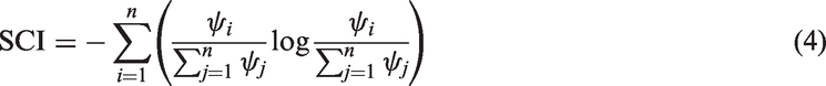
The effectiveness of a load path is measured as the ratio between the deformation work in the original structure and the deformation work performed on the statically determinate structure, that is, the fundamental structure. This ratio is called performance ratio ψ and ranges from zero to one since the denominator is always larger than the numerator. These bounds represent, respectively, the limit cases in which the load path is not effective or vice versa. The number of fundamental structures and, consequently, of performance ratios, n, depends on the original scheme. The measure of the “amount” of information required to describe the structural behavior is based on the definition of information entropy stated by Shannon (1948). In particular, the structural complexity index (SCI), is represented by

SCI = - \sum_{i = 1}^{n} (ψ_{i} \sum_{j = 1}^{n} ψ_{j} \log ψ_{i} \sum_{j = 1}^{n} ψ_{j})

(4)

The base of the logarithm is not relevant (if two, the measure is in bits). The entropy measure possesses many interesting properties (Gray, 2011). The identification of the load paths can be easily performed if the structural scheme is studied under the framework of Graph Theory (De Biagi and Chiaia, 2013).

In order to compare the complexities of various structures with different size and element numbers, a normalized parameter is introduced. The SCI is divided by its maximum possible value, which represents the situation in which each possible load path has the same effectiveness (i.e. the same performance factor). This situation, representing the maximum complexity corresponds to a SCI equal to log n, where n is the number of load paths. Thus, the normalized structural complexity index (NSCI) is expressed as

NSCI = SCI \log n

(5)

The NSCI ranges between zero and one. As the parameter approaches 0⁺, the structural system is simple. On the other hand, values of NSCI tending to 1⁻ refer to complex structures (De Biagi and Chiaia, 2013).

Physically speaking, maximum complexity, that is, maximum disorder, can be intended as white noise, which is a constant power spectral density signal, in the range of the spectrum between zero and one. Minimum complexity is gained by a simple harmonic oscillation, which representation in a spectral plot is a Dirac delta function at 1/n, as shown in Figure 2.

Figure 2.

Plot of the spectrum of white noise (thin line, i.e. the uniform plateau between 0 and 1) and of a simple harmonic oscillation (thick line, i.e. the Dirac delta function at 1/n) on a Frequency versus Intensity plot.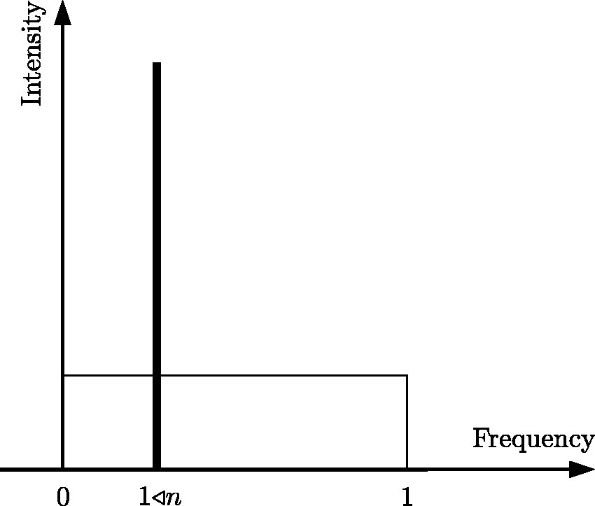

Damage on systems made of rods: Effects of stiffness variation

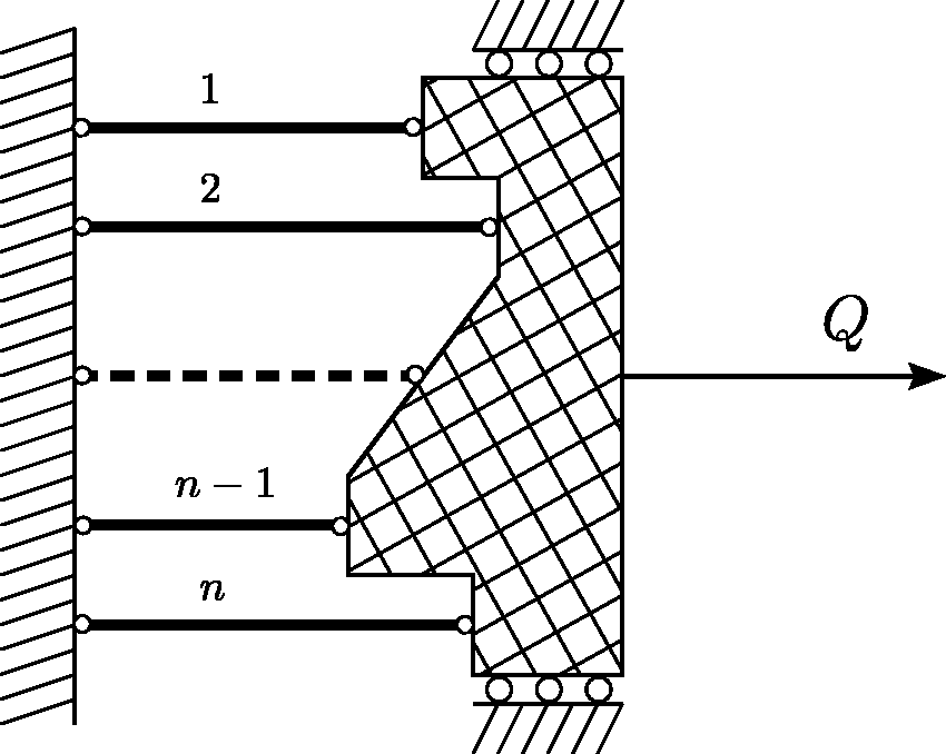
Consider a system of linear elastic rods working in parallel, as shown in Figure 3. The structure is composed of n rods: they are connected, on their right-hand side ends, to a rigid body to which a force Q is applied. Left-hand side ends are constrained and, thus, their displacements are prohibited. The movement of the rigid body is externally restricted in such a way that no rotational effects occur. That is, the point of application of Q is not relevant. Following the application of the external force, the system displaces. The force on each rod, N_i, is proportional to its axial stiffness, k_i, and to its elongation, δ_i, which is equal for all elements since the rigid body cannot be deformed nor rotated. Therefore, δ_i = δ and, thus

\dots

(6)

Figure 3.

Sketch of the system made of parallel rods (thick lines). The infinitely stiff element is the dashed line.

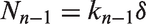
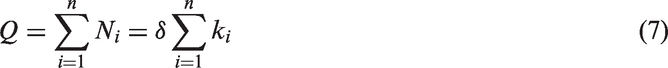
For the static equilibrium of the rigid body, the sum of the axial forces on the rods, ∑_iN_i, is equal and opposite to force Q. Summing member contributions of equations (6), the total force is equal to

Q = \sum_{i = 1}^{n} N_{i} = δ \sum_{i = 1}^{n} k_{i}

(7)

The term

\sum_{i = 1}^{n} k_{i}

is defined as the system equivalent stiffness, k_eq. The displacement is calculated from equation (7) as

δ = Q k_{eq}

(8)

The elastic work of deformation of the system of rods, W, is computed through Clapeyron's Theorem and is expressed as

W = 12 Q δ = 12 Q^{2} k_{eq}

(9)

In general, a variation of the stiffness of one of the rods implies a variation of the system equivalent stiffness and, thus, a change in the elastic work of deformation. The variation of the elastic work of deformation, ∂W, due to a variation of the stiffness of the qth rod, ∂k_q, is computed by differentiating equation (9) and is equal to

\partial W \partial k_{q} = - 121 k_{eq}^{2} Q^{2}

(10)

Since the components of the previous expression are squared quantities, the variation is negative, that is

\partial W \partial k_{q} < 0

(11)

showing that a decrease in stiffness produces increments of the work of deformation, W.

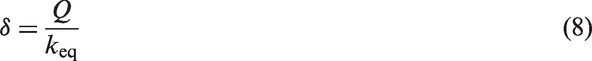
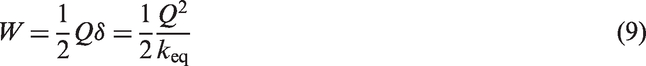
Note that the previous considerations relate to systems onto which the applied force is constant throughout all the damage process. In the case of fixed displacement, a decrease of the stiffness of one rod, for example, due to softening, implies a reduction of W.

Progressive removal of one rod

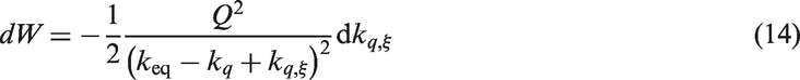
Progressive element removal can be intended as a progressive decrease of stiffness of the element from its initial value to zero (i.e. damage spreading). Supposing that the external force, Q, stays equal during the entire damage process, equation (8) can be differentiated with respect to k_q showing that

\partial δ = - Q k_{eq}^{2} \partial k_{q}

(12)

that is, the displacement of the rigid body progressively increases as much as the stiffness reduces.

In order to study the evolution of the deformation work during the damage process, the variation of stiffness can be controlled by a damage variable, ξ, ranging between zero, when the rod has its original stiffness, and one, when the element is totally removed (i.e. element failure), in accordance with the approach of Lemaître and Chaboche (1994). The stiffness of rod q, k_q,ξ, which is supposed to vary, is

k_{q, ξ} = k_{q} (1 - ξ)

(13)

where k_q is its initial value. Rearranging equation (10), the following differential expression is found

dW = - 12 Q^{2} (k_{eq} - k_{q} + k_{q, ξ})^{2} d k_{q, ξ}

(14)

Integrating equation (14) between the undamaged and damaged situation gives

\int_{W_{0}}^{W_{ξ}} d W = - Q^{2} 2 \int_{k_{q}}^{k_{q} (1 - ξ)} 1 (k_{eq} - k_{q} + k_{q, ξ})^{2} d k_{q, ξ}

(15)

where W₀ and W_ξ are the works of deformation in the undamaged scheme and at a generic damage situation ξ, respectively. The evolution of W with the damage ξ is thus defined as

W_{ξ} = 12 Q^{2} k_{eq} - k_{q} ξ

(16)

Note that the increase of deformation work is not linear, since the damage parameter ξ is at the denominator. The initial slope of W_ξ, expressed as

(d W_{ξ} d ξ)_{ξ = 0} = 12 Q^{2} k_{q} k_{eq}^{2}

(17)

and the concavity of the function

d^{2} W_{ξ} d ξ^{2} = 12 Q^{2} k_{q}^{2} (k_{eq} - k_{q} ξ)^{3}

(18)

are both positive quantities because of the positiveness of the stiffness.

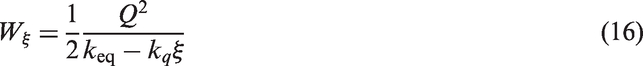
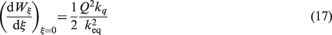
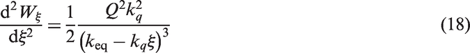
Consider a system of axes in which the damage parameter ξ is measured on the abscissa and the deformation work on the ordinate, see Figure 4. With the first and the second derivatives positive, the plot of W_ξ, in red in Figure 4, is below the straight line connecting the points (0,W₀) and (1,W₁), corresponding to the undamaged case and to the situation in which the qth rod is totally removed. The slope of this line can be computed as

W_{1} - W_{0} 1 - 0 = Q^{2} 2 (1 k_{eq} - k_{q} - 1 k_{eq}) = Q^{2} 2 k_{q} k_{eq} (k_{eq} - k_{q})

(19)

Since the damaged situation corresponds to a unitary value of the damage variable, equation (19) corresponds to the difference Δ_q between the deformation works, see Figure 4.

Figure 4.

Plot of W_ξ with damage evolution.

Remembering that W₀ = Q²/(2k_eq) and the grouping term k_q/k_eq, equations (17) and (19) can be rewritten as

(d W_{ξ} d ξ)_{ξ = 0} = W_{0} (k_{q} k_{eq})

(20)

and

Δ_{q} = W_{0} (k_{q} / k_{eq}) [1 - (k_{q} / k_{eq})]

(21)

Since k_q/k_eq < 1, the denominator of equation (21) is smaller than one and thus the following inequality holds

Δ_{q} > (d W_{ξ} d ξ)_{ξ = 0}

(22)

meaning that W_ξ is convex.

Performance and complexity of systems with parallel rods

De Biagi and Chiaia (2013) defined the concept of performance ratio, ψ. Referring to a scheme of parallel rods, one easily recognizes that a single rod represents a fundamental structure in itself. In other words, the qth fundamental structure is exclusively composed of rod q. The work of deformation performed on this fundamental structure is thus equal to

W_{S_{q}} = 12 Q^{2} k_{q}

(23)

That is, the performance factor of the qth fundamental structure (i.e. the one of the qth rod), remembering that W₀ = W, is

ψ_{q} = W_{0} W_{S_{q}} = Q^{2} 2 k_{eq} 2 k_{q} Q^{2} = k_{q} k_{eq}

(24)

One can easily note that the performance ratio is equal to the quantity grouped in the round brackets of equations (20) and (21). These equations can be rewritten as

(d W_{ξ} d ξ)_{ξ = 0} = W_{0} ψ_{q}

(25)

and

Δ_{q} = W_{0} ψ_{q} 1 - ψ_{q}

(26)

respectively.

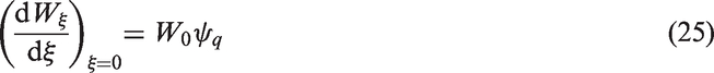
Analyzing equation (25), since the initial deformation work, W₀, is independent of rod q, that is, equal for any removed rod, the slope of the plot of Figure 4 is larger for structures that have a high performance ratio. Equation (26) can be rewritten as

Δ_{q} W_{0} = ψ_{q} 1 - ψ_{q}

(27)

Remembering that Δ_q is the difference between the work of deformation of damaged and undamaged schemes, equation (27) gives a measure of the relative increment of deformation work due to the removal of rod q. Large increments correspond to low robustness (i.e. to high sensitivity to damage). The system is considered robust if the effect of the removal of a single element does not imply a disproportionate increase of the deformation work.

Damage tolerance

The performed analysis considered the removal of a specific rod. It may now be interesting to measure the average effect of removing a single arbitrary rod of the structural system. We thus define the quantity

M = 1 n \sum_{i = 1}^{n} Δ_{i} W_{0}

(28)

as an average of the effects of the (alternate) removal of a generic rod on the scheme. Substituting equation (27) into equation (28) one gets

M = 1 n \sum_{i = 1}^{n} ψ_{i} 1 - ψ_{i}

(29)

deriving that the average importance of rod removal is a function of the way the total stiffness is distributed across the rods. Few considerations on equation (29) can be drawn. The minimum value of M, that is M^min, is attained when the performance ratios are equal. This assertion is proved in Appendix 1. This means that (i) the deformation works of any fundamental structure,

W_{S_{i}}

, are equal and (ii), as a consequence of parallel arrangement, that all the stiffnesses are equal. In other words, considering that

ψ_{1} = ψ_{2} = \dots = ψ_{n} = ψ

(30)

equation (29) can be rewritten as

M^{\min} = 1 n \sum_{i = 1}^{n} ψ 1 - ψ = 1 n [n ψ 1 - ψ] = ψ 1 - ψ

(31)

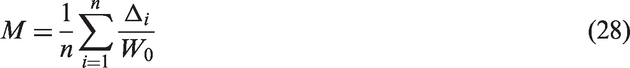
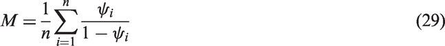
On the other hand, supposing that all the performance ratios ψ except one are close to zero, the value of M tends to infinite, as proved in Appendix 2.

The statistics of the performance ratios of the structure are of interest for the metrics of structural complexity discussed previously. Shannon (1948) proved that the maximum information entropy occurs when the probabilities of occurrence of any possible outcome are equal. Remembering the process that led to the computation of structural complexity (see De Biagi and Chiaia, 2013), for further details), the condition expressed by equation (30), that is, M^min, necessarily implies

NSCI = 1

(32)

that is, to the maximum structural complexity. Similarly, the condition expressed by equations (47) and (48), that is, M^max, is equivalent to

NSCI = 0

(33)

that is, to the minimum structural complexity.

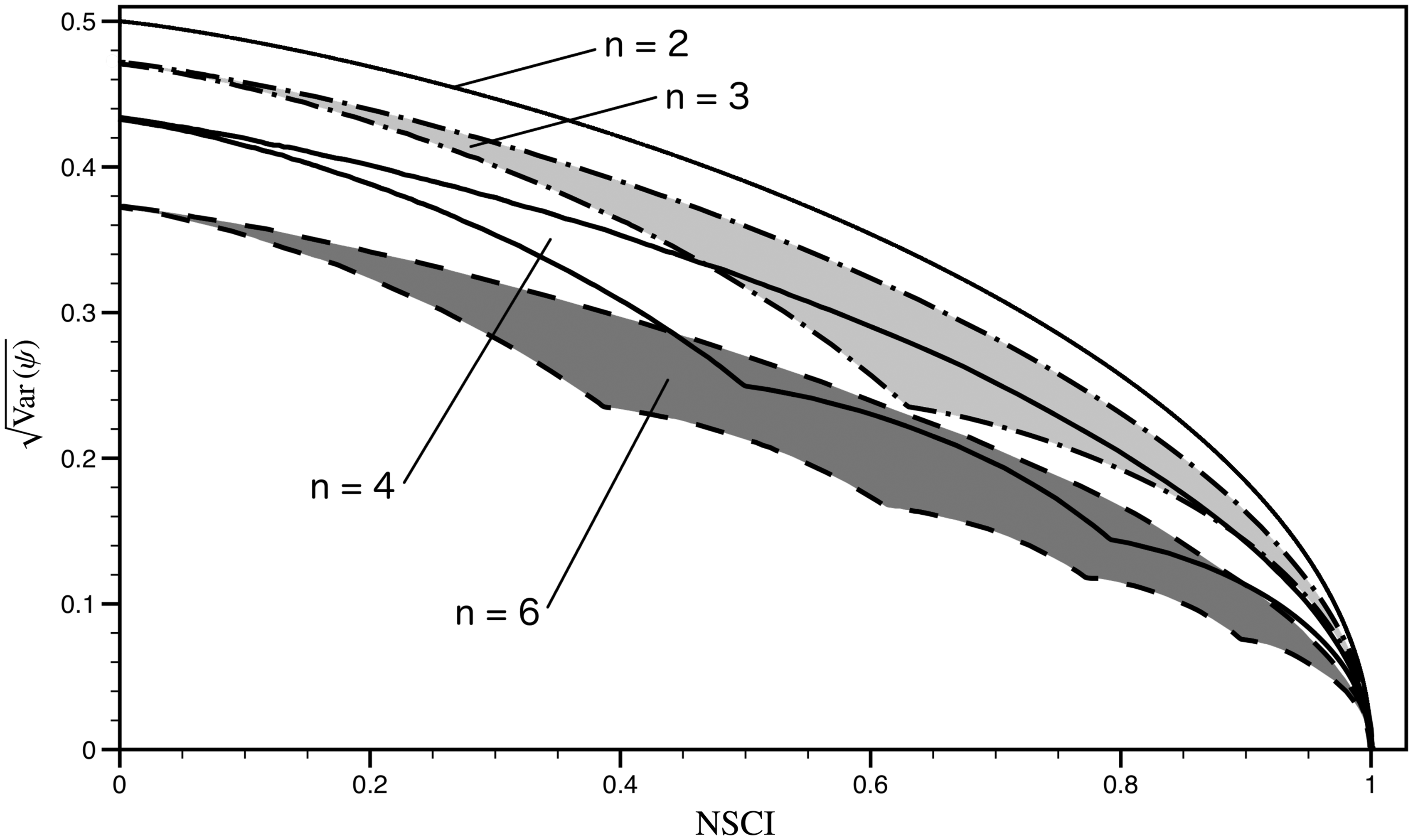
Performance ratios variance and structural complexity

In probability theory, variance and entropy both represent uncertainty about the value of a random variable (Zidek and van Eeden, 2003). Ebrahimi et al. (1999) classified continuous and discrete probability distribution by the effects of parametric variation on variance and entropy. Although different arrangements were shown, a not agreeing situation was determined. In more general terms, when getting information from observations, the variance can be referred to the uncertainty before the experiment, while the entropy is related to the uncertainty after the test (Arndt, 2001).

We try to turn such results in the framework of structural complexity in which the number of fundamental structures and, by consequence, performance ratios is finite and countable. At present, there are no direct links between the variance of the performance ratios and the NSCI. The former statistical variable measures how far the set of performance ratios is spread out. On the contrary, the NSCI, which is entropy based, can be intended as a measure of uncertainty (Arndt, 2001). In other words, consider a fundamental structure and compute its performance ratio. How uncertain is the value of the performance ratio of another fundamental structure, chosen at random? A measure of the uncertainty is represented by the NSCI. The gain of structural complexity reduces the uncertainty before the second measurement. As a limit, in the case of unitary NSCI, all the fundamental structures have the same performance ratio. No uncertainty is thus present on the performance ratio of the second structure after the computation of the same parameter on the first one.

In studying the complexity of rod systems, following the results proposed by the authors (De Biagi and Chiaia, 2013), the maximum structural complexity corresponds to the case reported in equation (30), when the mean of the performance ratios, μ(ψ), is equal to 1/n and the variance is equal to zero since all the terms have equal value. On the other hand, following the properties of information entropy stated by Shannon (1948) in his milestone paper, the minimum structural complexity is theoretically found if and only if all the performance ratios but one are zero, this one having the unit value (the mean of the performance ratios is 1/n). Since a rod is a physical connection, the stiffness has to be greater than zero. Although small, the corresponding fundamental structure performs a small finite deformation work, ζ, that is

and the variance, Var(ψ), can be easily determined as

Var (ψ) = 1 n lim_{ζ \to 0} [(n - 1) (ζ - 1 n)^{2} + (1 + (n - 1) ζ - 1 n)^{2}] = n - 1 n^{2}

(36)

Table 2 reports the variance of systems of parallel rods of various size.

Table 2.

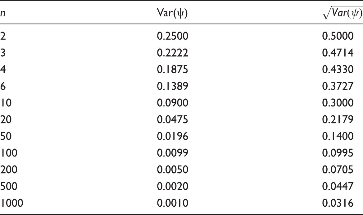
Theoretical variance of the performance ratios at zero complexity.

n	Var(ψ)	$\sqrt{Var (ψ)}$
2	0.2500	0.5000
3	0.2222	0.4714
4	0.1875	0.4330
6	0.1389	0.3727
10	0.0900	0.3000
20	0.0475	0.2179
50	0.0196	0.1400
100	0.0099	0.0995
200	0.0050	0.0705
500	0.0020	0.0447
1000	0.0010	0.0316

Numerical simulations

In the past sections, some analytical findings have been reported. Herein, numerical simulations are proposed. Their aim is essentially to present the trends of the variables previously treated, that is, the variance and M, in the range NSCI = (0;1). Before going further, it is important to note that:

the complexity index of a structure can be computed only after its mechanical/geometric properties and loading conditions are assigned, and not vice versa. Hence, the process of generating structures and computing their complexity is univocal (De Biagi, 2014).

In particular, in linear systems, as detailed in De Biagi and Chiaia (2014):

scaling of the load magnitude does not produces a variation on NSCI;

scaling of the system geometry does not produce a variation on NSCI if the load-set is exclusively composed by either forces or torques, that is, by external, size-independent loads;

scaling of system mechanical properties (Young's Modulus) does not produce a variation on NSCI.

As a result of the previous considerations, once the number of rods, n, has been defined, a Monte Carlo simulation can be performed following the steps listed below.

Sample the stiffness k_i of n − 1 rods. In reference to the previous considerations, in order not to consider similar but scaled systems, rod no.1 has the same reference stiffness for each simulation. Stiffness sampling is done through a random number generator and a reference maximum stiffness (assumed to be 20 times the stiffness of rod no.1).

Load the system with a unitary force Q = 1 and compute the corresponding work of deformation, the performance ratios and the complexity indices with equations (9), (24), (4) and (5) respectively.

Compute the variance as

Var (ψ) = 1 n \sum_{i = 1}^{n} (ψ_{i} - 1 n)^{2}

(37)

and M with equation (29).

The previous steps represent one simulation. Thousands of various simulations have been performed in order to cover the widest possible range of complexity levels, as detailed in the following.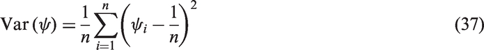

Variance

The behavior of the statistical variance at various complexity levels is now analyzed. In order to highlight the trends between the normalized structural complexity and the variance of performance ratios, Figure 5 is plotted. The X-axis relates to NSCI while $\sqrt{Var (ψ)}$ is presented on the Y-axis. The results of each simulation, taken as a couple of coordinates on the diagram, can be drawn as a point on the plot.

Figure 5.

Structural scheme made of four parallel rods. Plot of the variance of the performance ratios as a function of the normalized structural complexity index (NSCI). Each point corresponds to one of the 50,000 simulations. Notice the arc-type lower bound and the two singular points.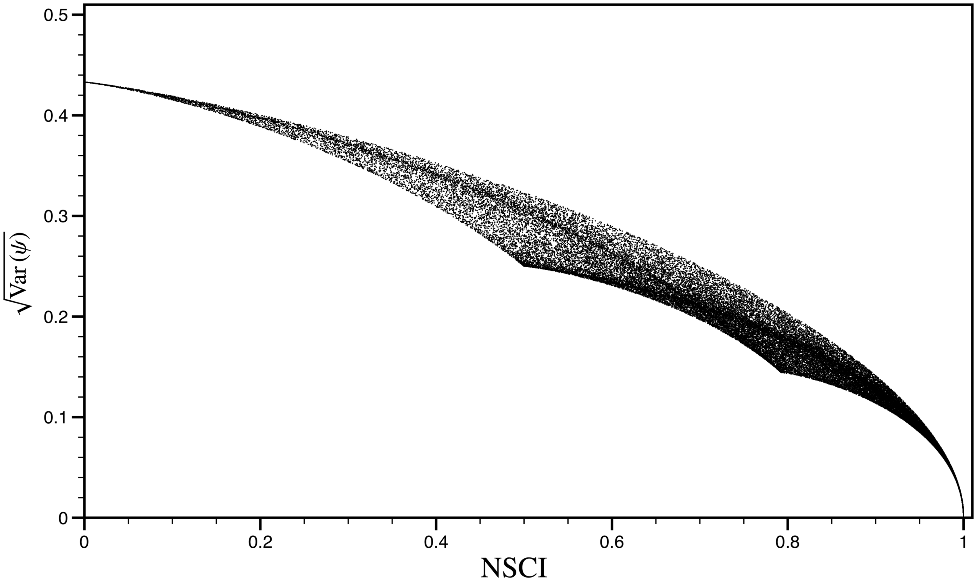

The scatter plot illustrated in Figure 5 relates to a structure made of four parallel rods, that is, n = 4. Fifty-thousand simulations have been performed. The analysis of the plot confirms some theoretical findings. That is, at NSCI ≈ 0 and NSCI = 1, the $\sqrt{Var (ψ)}$ tends to 0.43 and is null, respectively. The correct analytical value, that is, 0.4330, is reported in Table 2. The decrease of the variance is obtained as the complexity increases. In particular, two features are clearly visible.

There is no uniqueness in the relationship between complexity and variance. In other words, except for the bounds (i.e. NSCI = 0 and 1), at a given value of NSCI, a range of variances corresponds and vice versa. This behavior can be easily explained remembering that the structural complexity measure is an entropy-based measure: various probability distributions (i.e. with different second-order central moments) with equal probabilistic entropy exist. This idea is supported by Shannon's entropy power inequality (Shannon, 1948), which permits one to state that, for a given entropy, among all the possible continuous probability distributions, the normal probability distribution is the one that has minimum variance.

The scatter points cover an area whose upper bound is defined by a unique curve, while the bottom bound is represented by three arc-type curves and two singular points.

A similar test has been performed on a structural scheme made of 10 rods working in parallel (n = 10), as shown in Figure 6. In this situation, the arc-type lower bound is visible at low complexities: as much as NSCI increases, the lower bound tends to be a continuous curve.

Figure 6.

Structural scheme made of 10 parallel rods. Plot of the variance of the performance ratios as a function of the normalized structural complexity index. Each point corresponds to one of the 20,000 simulations.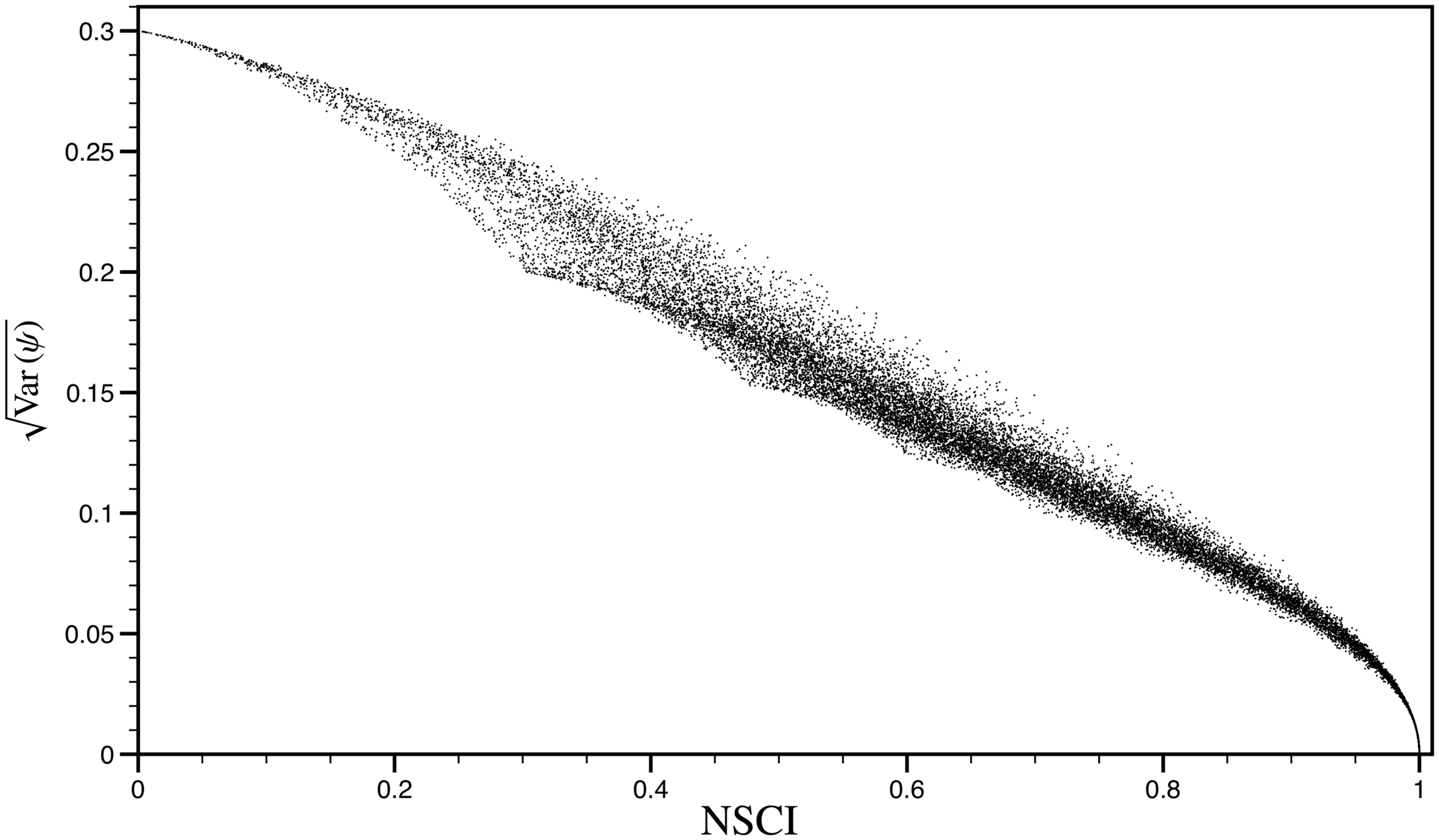

The clouds of points in each of the previous figures encompass an area of the diagram. In Figure 7, the areas related to structures made of different number of rods (n equal to 2, 3, 4 and 6) are compared. The upper bound is always defined by a unique curve. The lower bound is defined by arc-type curves. In case of n = 2 the relationship between structural complexity and variance is expressed as

- NSCI \log 2 = (12 + \sqrt{Var}) \log (12 + \sqrt{Var}) + (12 - \sqrt{Var}) \log (12 - \sqrt{Var})

(38)

The number of arches depends on the number of rods in the structural scheme and is equal to n − 1. In addition, in each case, the bounds have equal tangents at the ends, that is, at the minimum and maximum complexity, respectively. The slope of the tangents at the ends is thus constant even for structures with different numbers of rods.

Figure 7.

Plot of the areas encompassing the clouds of points related to structural schemes with 2, 3, 4 and 6 rods, respectively.

In the case of n = 2, the cloud of points is not present because there is a unique lower bound coincident with the upper one. As much as the number of elements increases, the singularities on the lower bound tend to disappear, see Figure 6 which relates to a structural scheme made of 10 rods (n = 10).

M-value

A similar approach has been followed for studying the behavior of the M-parameter for various complexity levels. As found in the previous paragraphs, at zero complexity, that is, NSCI = 0, the consequences of the removal of an element are significant: M tends to infinite. On the contrary, when NSCI = 1, M depends on the performance ratio, that is, a function of the number of rods in the structural system. In other words, substituting ψ with 1/n, equation (31) turns into

M = 1 n - 1

(39)

Figure 8 plots the M-values and the corresponding complexity indexes for various structural systems made of a different number of parallel rods. In particular, the results pertaining to schemes with two and four rods refer to a set of 50,000 simulations; the results pertaining to schemes with 10 rods refer to a set of 20,000 simulations. The following considerations can be drawn. Similar to what was discussed for the variance analysis presented in the previous paragraph, a cloud of points comes out of the simulations performed. In particular, M decreases as the complexity increases. Referring to the cloud of points and to the encompassing area, the upper bound is again a continuous curve while the lower bound can be identified by a multi-arch-type line. As already shown, the number of arches is n − 1, as previously detailed (i.e. the number of singularities is n − 2). Thus, for a given value of NSCI, a range of M is found.

Figure 8.

M-values at various complexities related to structural schemes with 2, 4 and 10 rods, respectively.

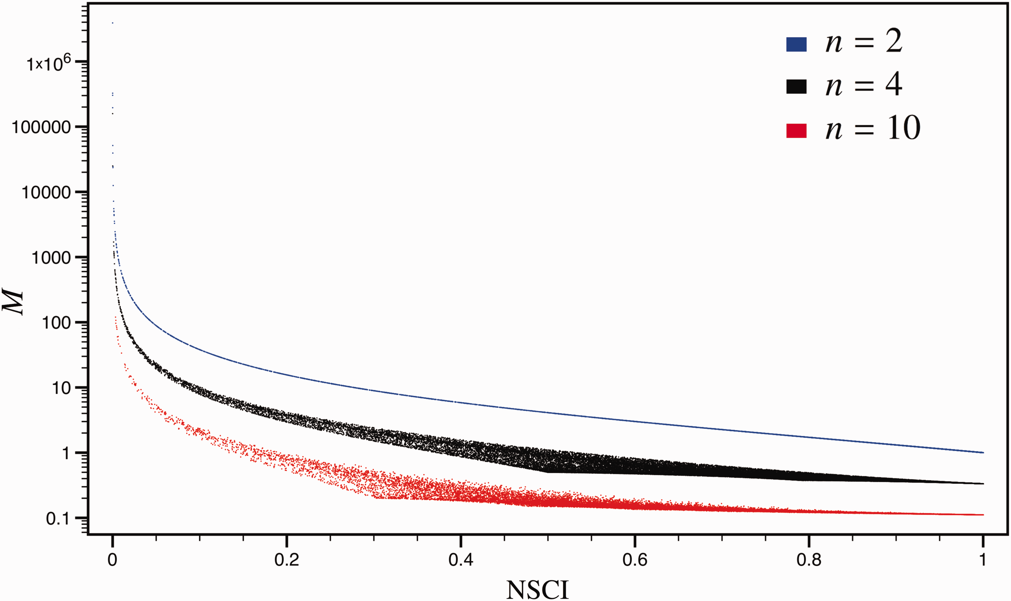
Looking to maximum complexity ranges and to the areas encompassing the cloud of points of Figure 8, the upper bound lines have equal slope in a semi-log reference system, independently of the number of rods. At very low complexities, they show a power-like behavior with power exponent equal to − 1.069.

Discussion

Following the analytical and numerical analyses, a series of considerations may be drawn. Note that, since the number of elements in the system is fixed, the statistical analysis of the performance ratios can always be done.

First, the power of the structural complexity metric is highlighted. The mean value of the performance ratios is always equal to the inverse of the number of the elements, independent from the values of the performance ratios. On the contrary, the variance has been shown to vary depending on the size of the system. In other words, at maximum complexity, the variance is always null, while at minimum complexity its value is proportional to the inverse of the number of elements. As the system increases its size, the variance tends to zero. Numerical simulations have confirmed that the variance is represented by unique (but different) quantities at minimum and maximum complexity, respectively. Hence, due to the extreme variability of the variance, the NSCI has to be preferred for the evaluation of the scattered values of the performance ratios.

The behavior of complex systems under damage has been investigated at various stages. At the initial stage, that is, at the point when the stiffness of the system starts reducing its value, the effect of damage on the system increases more as the performance ratio related to the damaged element gets greater. In other words, if the presence of the (potentially damaged) element is preponderant in the overall behavior, a slight variation of its properties implies large consequences on the entire system. In the perspective of designing a robust system it is, thus, better to keep the performance ratios of all the load paths (herein coinciding with the rods) equal. At the final stage of damage, that is, when the element is totally removed, the impact on the system depends on the value of the complexity. As much as the complexity reduces, the average effect increases dramatically. As expected, the effect is larger in systems with a small number of elements, for which binary systems represent the worst case. The effects of the size of the system can be easily understood: the larger the number of elements, the higher possibility of redistribution exists. Comparing systems with different size, see Figure 8, similar values of M are shown at different values of the complexity index. For example, M = 10 is found for NSCI equal to 0.28 in case of a system made of two rods, 0.10 for systems with four rods and 0.03 for structural schemes with 10 elements. Therefore, as long as the system is large, the whole effects are restrained even if the performance ratios tends not to be equal, that is, under a low complexity level.

In the proposed framework, the progressive degradation of the whole structure, that is, considering the removal of two, three, …, n − 1 elements, can be handled in the same way as herein done for one damaged element. Independently from the number of damaged elements, the impact of damage would minimize as much as the complexity of the original structure would increase. On the contrary, the maximum impact is expected when the complexity is minimum.

The effects of “non totally removed” rods, that is, the damage parameters value is between zero and one, have been investigated, for example, in De Biagi (2014); De Biagi and Chiaia (2013). The redistribution of forces within the damaged structure has a trend similar to the one of Figure 4, that is, there is no linearity between the variation of damage parameter and the variation of internal forces in the rods.

In addition, it has to be noted that parameter M relates to the average impact upon the system of a random damage event. Recalling the considerations made on graphs by Albert et al. (2000), in simple but large structural systems, for example, in those situations when the equivalent stiffness is due to few elements, the removal of elements that do not contribute to the overall behavior does not increase significantly the work of deformation on the system. On the contrary, a targeted removal would imply large effects (recall, e.g. the behavior of scale-free networks under an attack to a “hub” node).

Conclusions

The effects of damage on parallel systems have been investigated. The novel metrics of structural complexity (De Biagi and Chiaia, 2013) have been used for defining the amount of interaction between the various elements working in parallel. The interaction is measured through the performance ratio, which represents the ratio between the value of a state function related to the system made of an entire set of elements and the value corresponding to the system made of a single element. In mechanical systems, the above function is the work of deformation. Damage tolerance has been measured by calculating the average impact of the removal of a single element. The impact is the relative increment in the deformation work.

In structural engineering, a practical application of the findings herein illustrated has been recently proposed by De Biagi (2016) and relates to the design of a steel truss: the sizes of elements are the outputs of a parametric analysis accounting for the minimization of the normalized structural complexity under an arbitrary loading scheme. It is shown that the effects of a random removal of a rod are minimized on the optimized truss. Anyway, in any damage situation, it is necessary to provide enough resistance to the undamaged elements. This can be achieved, for example, in steel structures, through high ductility and the strength of the structural elements. In structural mechanics, an extension of the proposed approach to continuous systems (say plates) is possible; it is necessary first to identify an appropriate definition of structural complexity for non-discrete systems.

The results found in the case of mechanical systems can be exploited in other disciplines. Recalling the initial example, the presence of various (and efficient) communication media working in parallel gives the possibility to broadcast news to the population even if there is an unexpected interruption in the chain of communication, resulting in system robustness. The future of the present research would interest the relationship between systems working in parallel and the ways to implement them in order to ensure a global robustness. This property is a fundamental prerogative of systems in order to sustain the effects of unexpected events without collapsing.

Footnotes

Declaration of Conflicting Interests

The author(s) declared no potential conflicts of interest with respect to the research, authorship, and/or publication of this article.

Funding

The author(s) received no financial support for the research, authorship, and/or publication of this article.

Appendix 1

Appendix 2

References

Albert

Jeong

Barabási

(2000) Error and attack tolerance of complex networks. Nature 406(6794): 378–382.

Arndt

(2001) Information Measures: Information and its Description in Science and Engineering; with 64 Figures, Berlin Heidelberg: Springer.

Aven

Renn

(2010) Risk Management and Governance. Concepts, Guidelines and Applications, Berlin Heidelberg: Springer.

Avizienis A (1967) Design of fault-tolerant computers. In: Proceedings of the November 14–16, 1967, fall joint computer conference, pp.733–743. New York: ACM.

Baker

Schubert

Faber

(2008) On the assessment of robustness. Structural Safety 30(3): 253–267.

Cascetta

(2001) Transportation Systems Engineering: Theory and Methods, Dordrecht: Springer.

CEN (2002) EN 1990 (Eurocode 0): Basis of structural design. Comité Européen de Normalisation.

Cennamo

Chiaia

De Biagi

(2014) Monitoring and compartimentalized structures. Journal of Applied Mathematics and Mechanics / Zeitschrift für Angewandte Mathematik und Mechanik 95(6): 638–648. DOI: 10.1002/zamm.201300091.

De Biagi V (2014) Complexity and robustness of structures against extreme events. PhD Thesis, Politecnico di Torino, Italy.

10.

De Biagi

(2016) Structural behavior of a metallic truss under progressive damage. International Journal of Solids and Structures 82: 56–64. DOI: http://dx.doi.org/10.1016/j.ijsolstr.2015.12.016.

11.

De Biagi

Chiaia

(2013) Complexity and robustness of frame structures. International Journal of Solids and Structures 50(22): 3723–3741.

12.

De Biagi

Chiaia

(2014) Scaling in structural complexity. Complexity 20: 57–63. DOI: 10.1002/cplx.21496.

13.

Ebrahimi

Maasoumi

Soofi

(1999) Ordering univariate distributions by entropy and variance. Journal of Econometrics 90(2): 317–336.

14.

Gans

King

Mankiw

(2011) Principles of Microeconomics, Boston: Cengage Learning.

15.

Gray

(2011) Entropy and Information Theory, Wien: Springer-Verlag.

16.

Krajcinovic

(1996) Damage Mechanics Vol. 41, Amsterdam: Elsevier.

17.

Landau

Lifshitz

(1959) Course of Theoretical Physics Vol 7: Theory and Elasticity, Pergamon Press.

18.

Leal Filho

Voudouris

(2013) Global Energy Policy and Security, London: Springer.

19.

Lemaître

Chaboche

(1994) Mechanics of Solid Materials, Cambridge: Cambridge University Press.

20.

Masoero

Wittel

Herrmann

(2010) Progressive collapse mechanisms of brittle and ductile framed structures. Journal of Engineering Mechanics 136(8): 987.

21.

Parham

(2009) The Immune System, New York: Garland Science.

22.

Shannon

(1948) A mathematical theory of communication. Bell System Technical Journal 27(July 1928): 379–423. .

23.

Simon

(1962) The architecture of complexity. Proceedings Of The American Philosophical Society 106(6): 467–482.

24.

Starossek

Haberland

(2011) Approaches to measures of structural robustness. Structure and Infrastructure Engineering 7(7): 625–631.

25.

Zidek

van Eeden

(2003) Uncertainty, entropy, variance and the effect of partial information. Lecture Notes-Monograph Series 42: 155–167. .