Total energy equivalence in constitutive modeling of multidissipative materials

Abstract

In the present work, the total energy equivalence hypothesis was applied in constitutive modeling of engineering materials. The approach originally developed for damaged materials, was extended to modeling not only damage but also other dissipative phenomena, like phase transformation, in a consistent manner. The proposed model was examined by means of parametric studies to show its ability to reflect different experimentally observed features of real materials.

Keywords

Constitutive modeling dissipative material plasticity damage phase transformation

Introduction

A multidissipative material is often characterized by a multiphase microstructure where each phase exhibits different mechanical properties, and the volume fraction of phases in the representative volume of the material may evolve. The evolution of damage, which is responsible for the material degradation, may be governed by different mechanisms in each phase: in brittle phases the stress state has the crucial influence on damage (Murakami, 2012), while in soft, ductile phases the damage state is mainly determined by plastic flow (Chaboche, 1999; Lemaitre, 1992).

The quantitative modeling of the inelastic material response has various formulations when considering the nonlinear domain and the complexity of the microstructural evolutions taking place in the material. Depending on the scale, different approaches may be used in order to describe an overall structural response of a structure on the macroscale.

In general, micromechanical models relate the macroproperties and the macroresponse of a structure to its microstructure. In such approach, a given dissipative phenomenon is discrete and stochastic, induced by a number of weakly or strongly interacting micro-rearrangements that influence the overall structural response. The micromechanical models have the advantage of being able to sustain heterogeneous structural details on the microscale and mesoscale and to allow a micromechanical evolution equations based on the accurate micro-rearrangement growth processes involved.

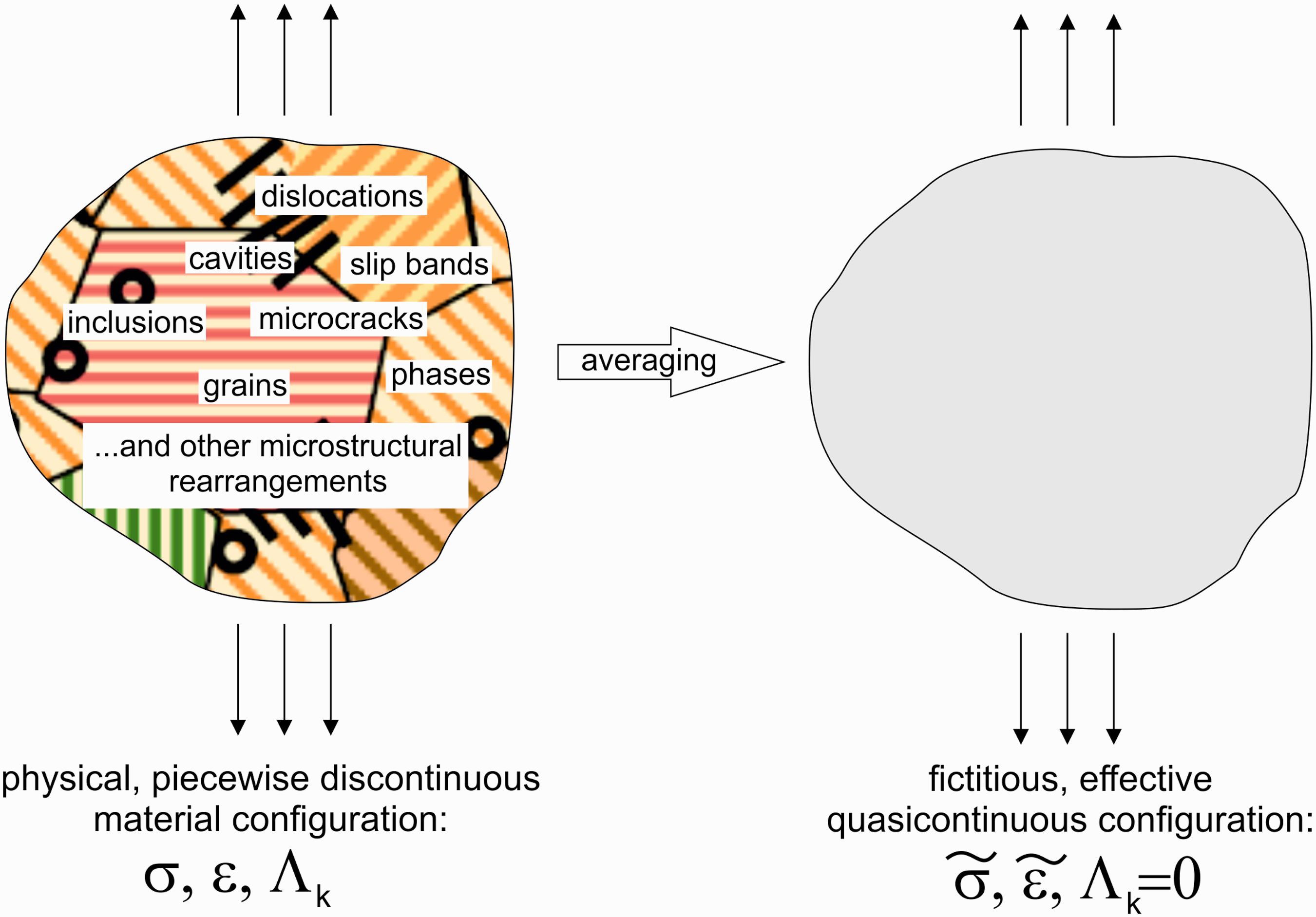
At the macrolevel the material heterogeneity (on the micro- and mesoscale) is smeared out over the representative volume element (RVE). When continuum mechanics approach is applied, the true state of the material within the RVE, represented by the topology, size, orientation, and number of micro-rearrangements, is mapped to a material point of the fictitious continuum (see Figure 1). The true distribution of microstructures and the correlation between them are measured by the change of the effective constitutive tensors (stiffness or compliance). The microstructural mechanisms are formalized at the continuum level by a suitable set of internal variables $Λ_{k}$ of the scalar, vectorial, or tensorial nature. The constitutive tensors for the dissipative material are defined by the use of even rank effect tensors (damage effect tensor, phase transformation effect tensor, etc.) that map thermodynamic forces from the physical (discontinuous and heterogeneous) to the fictitious (pseudo-continuous and pseudo-homogeneous) configurations.

Figure 1.

Physical (changed), and equivalent (pseudo-unchanged) continuum; the equivalence principles are used in order to smear out the true microchange distribution over the RVE to yield the effective constitutive modules for dissipative material. RVE: representative volume element.

The multiscale approach consists in proposing macroscopic constitutive equations taking into account the local behavior of each subphase in the RVE. The real difficulty is to establish a theoretical formalism linking macroscopic and microscopic scales when one or several subphases are nonlinear. Among some multiscale approaches proposing this link between scales, it is possible to distinguish three main categories:

Pure analytical approaches, mostly based on the work performed by Eshelby (1957) in elasticity. Within this framework, nonlinear materials are modeled through the linearization of Eshelby’s inclusion problem.

Integrated approaches, in which the final goal is to describe as close as possible the real microstructure of the RVE without macroscopic constitutive equations.

Sequential approaches (Chaboche et al., 2001, 2005; Kruch and Chaboche, 2011) generally performed in two steps, proposing analytical macroscopic constitutive equations which are determined from a previous multiscale analysis.

Both damage and phase transformation have been studied by many authors at various length scales:

At macrolevel continuum exhibits the effects of the phase mixture without resolving the details of the contributing phases. The most widely used macroscopic phase transformation models trace back to Leblond et al. (1989). Among more recent works are Fischer et al. (1996, 1998, 2000), Hallberg et al. (2007, 2010), Mahnken et al. (2012), Wolff et al. (2006, 2009), and others. Such approaches are naturally subjected to certain simplifying assumptions in order to provide practicable models for engineering problems.

At the meso- or phase-level the contributing phases are distinguished; however, the variant nature of the product phase only appears in an averaged sense.

At the microlevel single variants and their anisotropic shape changes become visible.

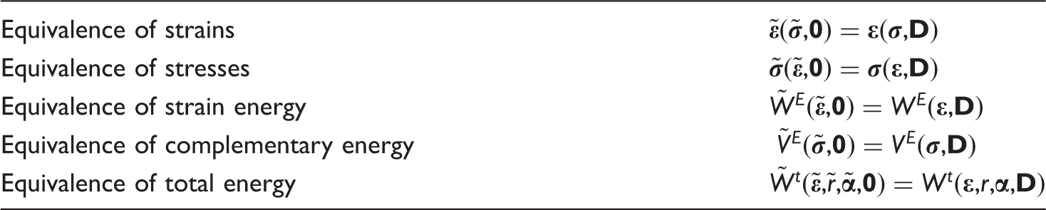
There are many papers covering the phase transformation phenomenon on the meso- or microlevel including multiscale approaches, for example Cherkaoui (2002), Fisher et al. (1997), Iwamoto (2004), Levitas and Ozsoy (2009), Mahnken et al. (2015).

In continuum damage mechanics the phenomenon of damage softening is described by the use of so-called effective state variables of a pseudo-undamaged quasicontinuum. To define these damage-effective state variables various equivalence hypotheses are formulated, for example: (a) strain equivalence hypothesis (Lemaitre, 1971; Lemaitre and Chaboche, 1978), (b) stress equivalence hypothesis (Simo and Ju, 1987), (c) strain energy or complementary energy equivalence hypotheses (Cordebois and Sidoroff, 1982a, 1982b), or finally (d) total energy equivalence hypothesis (Chow and Lu, 1992; Saanouni et al., 1994). According to these hypotheses, the effective state variables are defined in such a way that, respectively, strains, stresses, strain energy or complementary strain energy, or total energy for both real (damaged) and fictitious (pseudo-undamaged) materials are the same (see Table 1).

Table 1.

Hypotheses of mechanical equivalence used to define damage-effective state variables.

Equivalence of strains	$ε ~ (σ ~, 0) = ε (σ, D)$
Equivalence of stresses	$σ ~ (ε ~, 0) = σ (ε, D)$
Equivalence of strain energy	$W ~ E (ε ~, 0) = W E (ε, D)$
Equivalence of complementary energy	$V ~ E (σ ~, 0) = V E (σ, D)$
Equivalence of total energy	$W ~ t (ε ~, r ~, α ~, 0) = W t (ε, r, α, D)$

In the present work, we consider a material that is subjected not only to damage, but also to other dissipative phenomena, for example: plastic slips, phase transformation from the primary ductile matrix material to the secondary brittle inclusion material, and damage development in both phases. The constitutive description of such multidissipative material will be derived on the basis of total energy equivalence hypothesis, extended to all the dissipative phenomena regarded.

Constitutive model of a general dissipative material

State variables

Microstructural variables

In our constitutive modeling, performed under the assumption of small strains, we adopt the well-known formalism of thermodynamics of irreversible processes with internal state variables, and the local state method (Murakami, 2012; Saanouni, 2012). In this approach, the state of a material is entirely determined by certain values of some independent variables called variables of state. The irreversible rearrangements of the internal structure can be represented by a subset of state variables describing the current state of the material microstructure

{Λ k}, k = p, d, tr, \dots,

(1)

where

Λ k

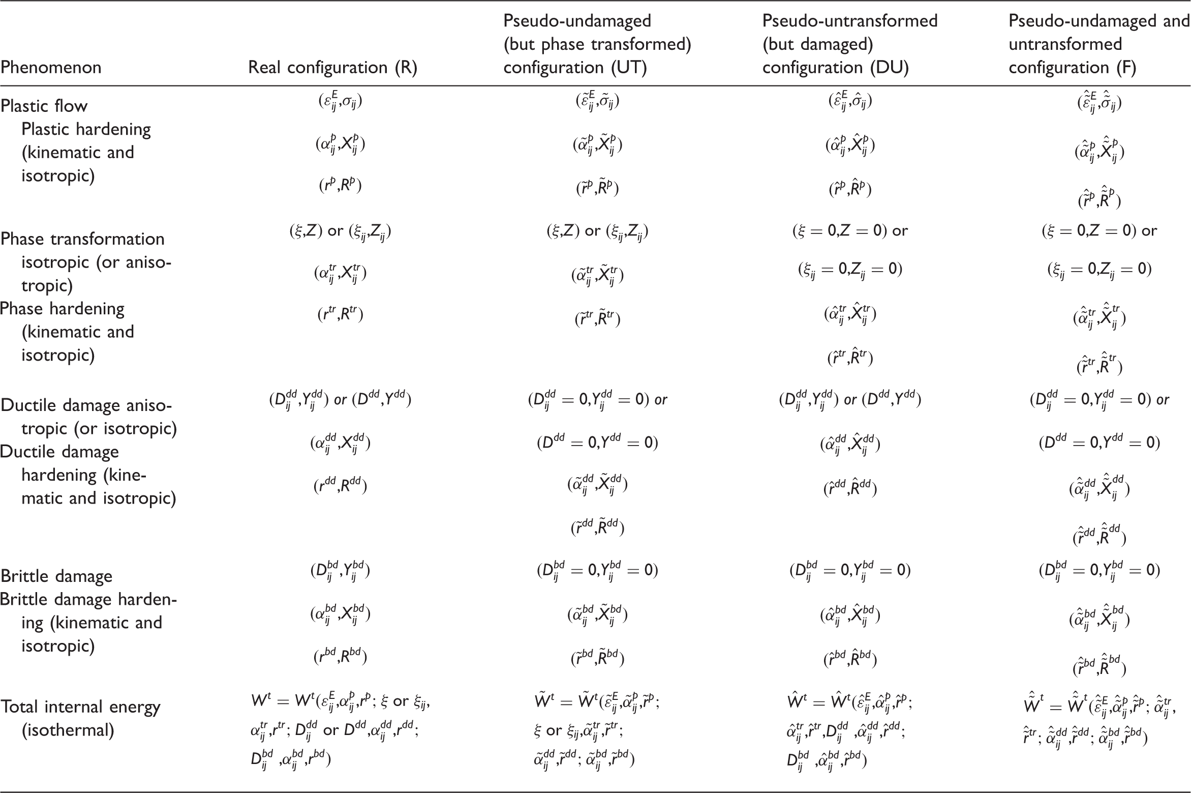
may be scalars, vectors, or even rank tensors, and index k denotes the dissipative phenomenon considered (p—plastic slips, d—damage,

tr

—phase transformation, etc.). Degradation in materials due to microcracks and microvoids is measured by the use of different metrics, for example the total crack area (or volume) related to the initial area (volume), degradation of the elastic modulus, change in density, etc. (cf. Chaboche, 1997; Egner, 2012; Ganczarski et al., 2010; Gomez and Basaran, 2006; Murakami and Ohno, 1981; Skrzypek and Kuna-Ciskal, 2003). For damage description, in the case where the damaged material remains isotropic, the current state of damage is often represented by the scalar variable

Λ d = D

denoting the volume fraction of cracks and voids in the total representative volume. Damage acquired orthotropy requires a second-order tensor, for example the classical Murakami and Ohno (1981) tensor. In the most general case of anisotropy, the description of damage needs to be embodied in an eight-order tensor (cf Cauvin and Testa, 1999), while the principle of strain equivalence allows using fourth-order tensors. For a multiphase material, different damage mechanisms (ductile or/and brittle) may be observed in material phases, therefore several separate damage variables may have to be used (cf. Egner et al., 2015a; see Table 2). It has been also shown that entropy production can be used as a damage metrics (cf. Basaran and Nie, 2004, 2007; Basaran and Yan, 1998; Gomez and Basaran, 2006; Li and Basaran, 2009; Yao and Basaran, 2013). Such approach provides a framework for all damage models, using entropy generation rate.

Table 2.

Pairs of variables related to different configurations defined in the model.

Phenomenon	Real configuration (R)	Pseudo-undamaged (but phase transformed) configuration (UT)	Pseudo-untransformed (but damaged) configuration (DU)	Pseudo-undamaged and untransformed configuration (F)
Plastic flow Plastic hardening (kinematic and isotropic)	$(ɛ_{ij}^{E}, σ_{ij})$ $(α_{ij}^{p}, X_{ij}^{p})$ $(r p, R p)$	$({ɛ ~}_{ij}^{E}, {σ ~}_{ij})$ $({α ~}_{ij}^{p}, {X ~}_{ij}^{p})$ $(r ~ p, R ~ p)$	$({ɛ \land}_{ij}^{E}, {σ \land}_{ij})$ $({α \land}_{ij}^{p}, {X \land}_{ij}^{p})$ $(r \land p, R \land p)$	$(~ \land ɛ_{ij}^{E}, ~ \land σ_{ij})$ $(~ \land α_{ij}^{p}, ~ \land X_{ij}^{p})$ $(~ \land r p, ~ \land R p)$
Phase transformation isotropic (or anisotropic) Phase hardening (kinematic and isotropic)	$(ξ, Z) or (ξ_{ij}, Z_{ij})$ $(α_{ij}^{tr}, X_{ij}^{tr})$ $(r tr, R tr)$	$(ξ, Z) or (ξ_{ij}, Z_{ij})$ $({α ~}_{ij}^{tr}, {X ~}_{ij}^{tr})$ $(r ~ tr, R ~ tr)$	$(ξ = 0, Z = 0) or$ $(ξ_{ij} = 0, Z_{ij} = 0)$ $({α \land}_{ij}^{tr}, {X \land}_{ij}^{tr})$ $(r \land tr, R \land tr)$	$(ξ = 0, Z = 0) or$ $(ξ_{ij} = 0, Z_{ij} = 0)$ $(~ \land α_{ij}^{tr}, ~ \land X_{ij}^{tr})$ $(~ \land r tr, ~ \land R tr)$
Ductile damage anisotropic (or isotropic) Ductile damage hardening (kinematic and isotropic)	$(D_{ij}^{dd}, Y_{ij}^{dd}) or (D dd, Y dd)$ $(α_{ij}^{dd}, X_{ij}^{dd})$ $(r dd, R dd)$	$(D_{ij}^{dd} = 0, Y_{ij}^{dd} = 0) or$ $(D dd = 0, Y dd = 0)$ $({α ~}_{ij}^{dd}, {X ~}_{ij}^{dd})$ $(r ~ dd, R ~ dd)$	$(D_{ij}^{dd}, Y_{ij}^{dd}) or (D dd, Y dd)$ $({α \land}_{ij}^{dd}, {X \land}_{ij}^{dd})$ $(r \land dd, R \land dd)$	$(D_{ij}^{dd} = 0, Y_{ij}^{dd} = 0) or$ $(D dd = 0, Y dd = 0)$ $(~ \land α_{ij}^{dd}, ~ \land X_{ij}^{dd})$ $(~ \land r dd, ~ \land R dd)$
Brittle damage Brittle damage hardening (kinematic and isotropic)	$(D_{ij}^{bd}, Y_{ij}^{bd})$ $(α_{ij}^{bd}, X_{ij}^{bd})$ $(r bd, R bd)$	$(D_{ij}^{bd} = 0, Y_{ij}^{bd} = 0)$ $({α ~}_{ij}^{bd}, {X ~}_{ij}^{bd})$ $(r ~ bd, R ~ bd)$	$(D_{ij}^{bd} = 0, Y_{ij}^{bd} = 0)$ $({α \land}_{ij}^{bd}, {X \land}_{ij}^{bd})$ $(r \land bd, R \land bd)$	$(D_{ij}^{bd} = 0, Y_{ij}^{bd} = 0)$ $(~ \land α_{ij}^{bd}, ~ \land X_{ij}^{bd})$ $(~ \land r bd, ~ \land R bd)$
Total internal energy (isothermal)	$W t = W t (ɛ_{ij}^{E}, α_{ij}^{p}, r p; ξ or ξ_{ij}, α_{ij}^{tr}, r tr; D_{ij}^{dd} or D dd, α_{ij}^{dd}, r dd; D_{ij}^{bd}, α_{ij}^{bd}, r bd)$	$W ~ t = W ~ t ({ɛ ~}_{ij}^{E}, {α ~}_{ij}^{p}, r ~ p; ξ or ξ_{ij}, {α ~}_{ij}^{tr}, r ~ tr; {α ~}_{ij}^{dd}, r ~ dd; {α ~}_{ij}^{bd}, r ~ bd)$	$W \land t = W \land t ({ɛ \land}_{ij}^{E}, {α \land}_{ij}^{p}, r \land p; {α \land}_{ij}^{tr}, r \land tr, D_{ij}^{dd}, {α \land}_{ij}^{dd}, r \land dd; D_{ij}^{bd}, {α \land}_{ij}^{bd}, r \land bd)$	$~ \land W t = ~ \land W t (~ \land ɛ_{ij}^{E}, ~ \land α_{ij}^{p}, ~ \land r p; ~ \land α_{ij}^{tr}, ~ \land r tr; ~ \land α_{ij}^{dd}, ~ \land r dd; ~ \land α_{ij}^{bd}, ~ \land r bd)$

For the phase transformation analysis, the scalar variable $Λ ph = ξ$ is commonly adopted, which denotes the volume fraction of the secondary phase in the RVE. However, a scalar variable is not capable of describing the acquired anisotropy due to a possible partially directional nature of the secondary inclusions in the matrix. Therefore, instead of scalar variable a second-order tensor can be defined in analogy to damage tensor (cf. Egner, 2012).

Hardening variables

Another subset of state variables consists of internal (hidden) variables corresponding to the modifications of yield surfaces

{h k} = {r k, α_{ij}^{k}, l_{ijpq}^{k}, g_{ijpqmn}^{k}}, k = p, d, tr, \dots,

(2)

where

r k

corresponds to isotropic expansion of the yield surface,

α_{ij}^{k}

affects translatoric displacements of the yield surface,

l_{ijpq}^{k}

is a hardening tensor of the fourth order which includes varying lengths of axes and rotation of the yield surface, and

g_{ijpqmn}^{k}

describes changes of the curvature of the yield surface (distortion) related to kth dissipative phenomenon (cf. Egner and Egner, 2015; Kowalsky et al., 1999).

The complete set of state variables ${V st}$ reflecting the current state of the thermodynamic system consists of observable variables: elastic (or total) strain tensor $ɛ_{ij}^{E}$ and absolute temperature θ, and two groups of microstructural ${Λ k}$ and hardening ${h k}$ state variables

{V st} = {ɛ_{ij}^{E}, θ; Λ k; h k}, k = p, d, tr, \dots,

(3)

Effective state variables

The rearrangements of a material microstructure affect its global mechanical properties either causing softening (for ex. damage) or hardening (for ex. transformation from soft to hard phase). This means that material behavior (both elastic and inelastic) is influenced by the microstructural mechanisms. To account for the influence of the dissipative phenomena on the global mechanical properties, the so-called effective state variables can be used in the state and dissipation potentials, instead of the classical state variables (equation (3)). We formulate the total energy equivalence hypothesis (H1) in the following way (cf. Saanouni et al., 1994):

(H1): At any time (t), to an RVE in its real (deformed, damaged, phase transformed, etc.) configuration, described by the set of state variable pairs, we associate a safe unchanged (undamaged, untransformed, etc.) equivalent fictive configuration, the state of which is described by the effective state variables—in such a manner that the total internal energy defined over the two (real and fictive) configurations is the same.

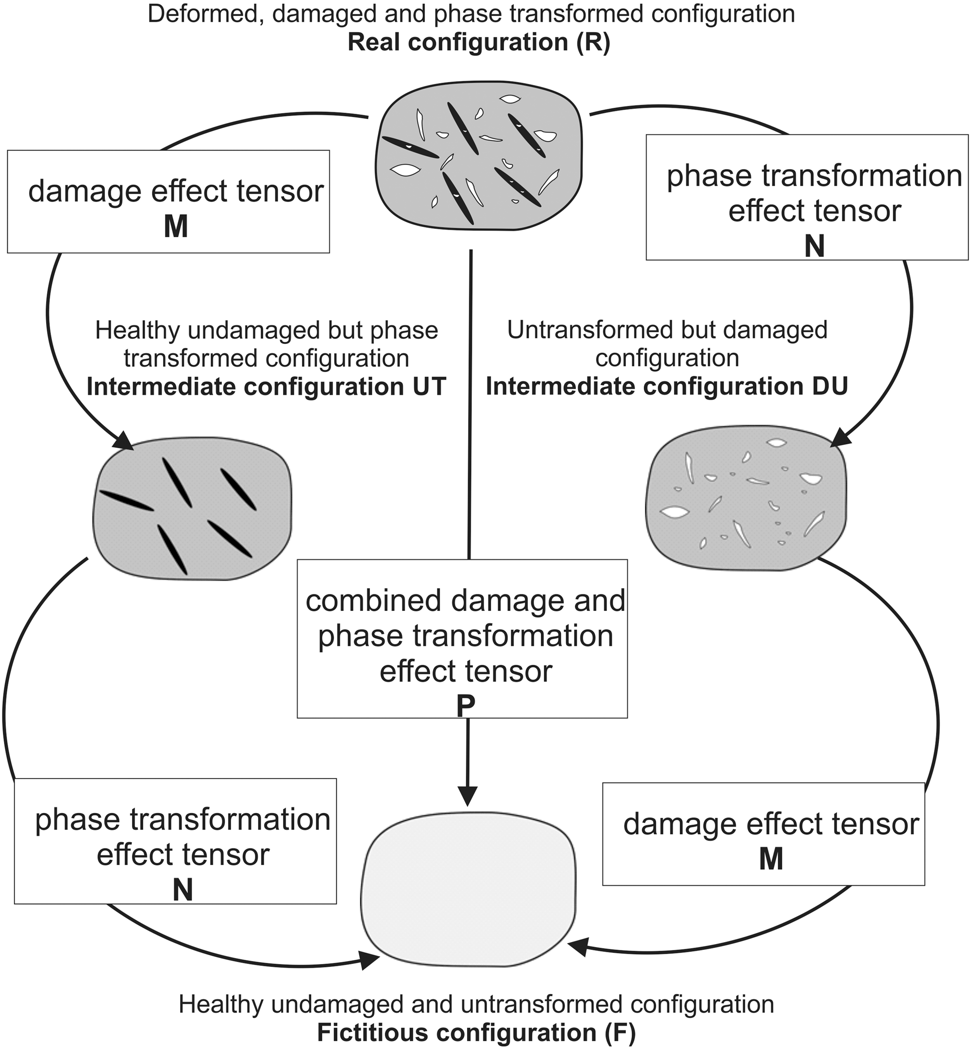
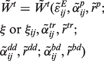
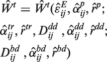
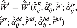
The definitions of effective state variables are related to different fictitious configurations introduced in the model. Let us consider a real, discontinuous, and heterogeneous configuration (R) of an exemplary material subjected to three dissipative phenomena: plastic slips, damage, and phase transformation (see Figure 2). We introduce a fictitious quasi-continuous and quasi-homogeneous configuration (F), characterized by the couples of effective state variables and effective thermodynamic forces (see Table 2) defined on the basis of the total energy equivalence hypothesis (H1). Mapping from configuration (R) to (F) may be equivalently performed with the use of two intermediate configurations: (UT), which is idealized undamaged but phase transformed, and (DU), which is damaged but idealized untransformed configuration (see Figure 2). Each intermediate configuration is characterized by the proper pairs of effective variables, defined on the basis of the total energy equivalence applied to the real configuration (R) and the intermediate configuration considered.

Figure 2.

Schematic representation of the total energy equivalence concept.

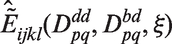
In the present paper, all the dissipative phenomena are therefore consistently considered at the macrolevel and described by the use of the same thermodynamic framework. The representative volume of a real, discontinuous (due to cavities and microcracks), and heterogeneous (due to phases, grains, inclusions, slip bands, dislocations, microstructures, cells, cavities, microcracks, etc.) material is mapped into a point of fictitious homogeneous continuum in which all the micro-rearrangements are smeared out without resolving the details of contributing components. When attempting to use a unified approach to damage and phase transformation, two “effect” tensors are defined: classical damage effect tensor (M_ijkl) that maps the state variables from the real damaged ( $σ_{ij}, ɛ_{ij}$ ) to fictitious pseudo-undamaged ( ${σ ~}_{ij}, {ɛ ~}_{ij}$ ) configuration, and a new phase transformation effect tensor (N_ijkl). This tensor maps the state variables from the real transformed ( $σ_{ij}, ɛ_{ij}$ ) to fictitious pseudo-untransformed ( ${σ \land}_{ij}, {ɛ \land}_{ij}$ ) configuration.

Mapping from the real damaged and transformed configuration (R) to fictitious pseudo-undamaged and pseudo-untransformed configuration (F) is therefore realized in two steps, leading to the definition of intermediate configurations (UT) and (DU). However, both steps are qualitatively different: the first one transforms a highly discontinuous configuration to a perfectly continuous one, while the second transforms a highly heterogeneous (multiphase) configuration to a perfectly homogeneous (mono-phase) configuration.

The general expression for the equivalence of total internal energy between subsequent configurations may be written in the following way

W t (ɛ_{ij}^{E}, α_{ij}^{p}, r p; ξ or ξ_{ij}, α_{ij}^{tr}, r tr; D_{ij}^{dd} or D dd, α_{ij}^{dd}, r dd; D_{ij}^{bd}, α_{ij}^{bd}, r bd) = W ~ t ({ɛ ~}_{ij}^{E}, {α ~}_{ij}^{p}, r ~ p; ξ or ξ_{ij}, {α ~}_{ij}^{tr}, r ~ tr; {α ~}_{ij}^{dd}, r ~ dd; {α ~}_{ij}^{bd}, r ~ bd) = W \land t ({ɛ \land}_{ij}^{E}, {α \land}_{ij}^{p}, r \land p; {α \land}_{ij}^{tr}, r \land tr; D_{ij}^{dd} or D dd, {α \land}_{ij}^{dd}, r \land dd; D_{ij}^{bd}, {α \land}_{ij}^{bd}, r \land bd) = ~ \land W t (~ \land ɛ_{ij}^{E}, ~ \land α_{ij}^{p}, ~ \land r p; ~ \land α_{ij}^{tr}, ~ \land r tr; ~ \land α_{ij}^{dd}, ~ \land r dd; ~ \land α_{ij}^{bd}, ~ \land r bd)

(4)

Hypothesis (H1) (4) will be further expressed in a stronger form that all the energy components, the reversible elastic energy $W E$ , kinematic hardening energy $W kin$ , and isotropic hardening energy $W iso$ , are equivalent

W E = \frac{1}{2} σ_{ij} ɛ_{ij}^{E} = \frac{1}{2} {σ ~}_{ij} {ɛ ~}_{ij}^{E} = \frac{1}{2} {σ \land}_{ij} {ɛ \land}_{ij}^{E} = \frac{1}{2} ~ \land σ_{ij} ~ \land ɛ_{ij}^{E}

(5)

W kin = \frac{1}{2} X_{ij}^{p} α_{ij}^{p} + \frac{1}{2} X_{ij}^{tr} α_{ij}^{tr} + \frac{1}{2} X_{ij}^{d} α_{ij}^{d} + \frac{1}{2} X_{ij}^{b} α_{ij}^{b} = \frac{1}{2} {X ~}_{ij}^{p} {α ~}_{ij}^{p} + \frac{1}{2} {X ~}_{ij}^{tr} {α ~}_{ij}^{tr} + \frac{1}{2} {X ~}_{ij}^{d} {α ~}_{ij}^{d} + \frac{1}{2} {X ~}_{ij}^{b} {α ~}_{ij}^{b} = \frac{1}{2} {X \land}_{ij}^{p} {α \land}_{ij}^{p} + \frac{1}{2} {X \land}_{ij}^{tr} {α \land}_{ij}^{tr} + \frac{1}{2} {X \land}_{ij}^{dd} {α \land}_{ij}^{dd} + \frac{1}{2} {X \land}_{ij}^{bd} {α \land}_{ij}^{bd} = \frac{1}{2} ~ \land X_{ij}^{p} ~ \land α_{ij}^{p} + \frac{1}{2} ~ \land X_{ij}^{tr} ~ \land α_{ij}^{tr} + \frac{1}{2} ~ \land X_{ij}^{dd} ~ \land α_{ij}^{dd} + \frac{1}{2} ~ \land X_{ij}^{bd} ~ \land α_{ij}^{bd}

(6)

W iso = \frac{1}{2} R p r p + \frac{1}{2} R tr r tr + \frac{1}{2} R dd r dd + \frac{1}{2} R bd r bd = \frac{1}{2} R ~ p r ~ p + \frac{1}{2} R ~ tr r ~ tr + \frac{1}{2} R ~ dd r ~ dd + \frac{1}{2} R ~ bd r ~ bd = \frac{1}{2} R \land p r \land p + \frac{1}{2} R \land tr r \land tr + \frac{1}{2} R \land dd r \land dd + \frac{1}{2} R \land bd r \land bd = \frac{1}{2} ~ \land R p ~ \land r p + \frac{1}{2} ~ \land R tr ~ \land r tr + \frac{1}{2} ~ \land R dd ~ \land r dd + \frac{1}{2} ~ \land R bd ~ \land r bd

(7)

A general solution that satisfies equation (5) may take the following form

{σ ~}_{ij} = [M_{ijkl}^{E} (D dd, D bd)] - 1 σ_{kl}

(8)

{σ \land}_{ij} = [N_{ijkl}^{E} (ξ)] - 1 σ_{kl}

(9)

~ \land σ_{ij} = [P_{ijkl}^{E} (D dd, D bd, ξ)] - 1 σ_{kl}

(10)

{ɛ ~}_{ij}^{E} = [M_{ijkl}^{E} (D dd, D bd)] T ɛ_{kl}^{E}

(11)

{ɛ \land}_{ij}^{E} = [N_{ijkl}^{E} (ξ)] T ɛ_{kl}^{E}

(12)

~ \land ɛ_{ij}^{E} = [P_{ijkl}^{E} (D dd, D bd, ξ)] T ɛ_{kl}^{E}

(13)

In the above equations, $M_{ijkl}^{E} (D dd, D bd)$ , $N_{ijkl}^{E} (ξ)$ , and $P_{ijkl}^{E} (D dd, D bd, ξ)$ are symmetric fourth-order operator functions of damage variables and/or phase transformation variable. These operators should exhibit certain characteristics. Namely, damage effect operator $M_{ijkl}^{E} (D dd, D bd)$ should

be positive definite, symmetric, and decreasing function of damage tensors;

be reduced to the fourth-rank unit tensor in the absence of damage, $M_{ijkl}^{E} (0, 0) = I_{ijkl} = \frac{1}{2} (δ_{ik} δ_{jl} + δ_{il} δ_{jk})$ ;

tend toward the fourth-order zero tensor at total fracture of the RVE when the average damage tensor approaches the unit tensor, $D_{ij}^{avg} = δ_{ij}$ . The simplest average damage tensor definition is given by equation (24).

Phase transformation effect operator $N_{ijkl}^{E} (ξ)$ should

be positive definite, symmetric, and monotonic function of phase transformation variable;

be reduced to the fourth-rank unit tensor in the absence of phase transformation, $N_{ijkl}^{E} (0) = I_{ijkl}$ ;

transform the properties of matrix material into the properties of the secondary phase when the phase transformation variable reaches unity.

The combined effect operator $P_{ijkl}^{E} (D dd, D bd, ξ)$ should

be positive definite, symmetric but not necessarily monotonic function of damage and phase transformation variables;

be reduced to the fourth-rank operator $M_{ijkl}^{E} (D dd, D bd)$ in the absence of phase transformation, and to the fourth-rank operator $N_{ijkl}^{E} (ξ)$ in the absence of damage: $P_{ijkl}^{E} (D dd, D bd, 0) = M_{ijkl}^{E} (D dd, D bd)$ , $P_{ijkl}^{E} (0, 0, ξ) = N_{ijkl}^{E} (ξ)$ .

For each of kinematic hardenings it is assumed here that:

(A1) A given dissipative phenomenon affects all kinematic hardening variables related to another dissipative phenomenon in the same way. However, this influence may be different for different dissipative phenomena. In particular, we assume here that a given dissipative phenomenon does not affect itself.

Therefore

{X ~}_{ij}^{k} = [M_{ijpq}^{k, kin} (D dd, D bd)] - 1 X_{pq}^{k}, {α ~}_{ij}^{k} = [M_{ijpq}^{k, kin} (D dd, D bd)] T α_{pq}^{k}

(14)

{X \land}_{ij}^{k} = [N_{ijpq}^{k, kin} (ξ)] - 1 X_{pq}^{k}, {α \land}_{ij}^{k} = [N_{ijpq}^{k, kin} (ξ)] T α_{pq}^{k}

(15)

~ \land X_{ij}^{k} = [P_{ijpq}^{k, kin} (D dd, D bd, ξ)] - 1 X_{pq}^{k}, ~ \land α_{ij}^{k} = [P_{ijpq}^{k, kin} (D dd, D bd, ξ)] T α_{pq}^{k}

(16)

where index

k = p, tr, dd, bd, \dots,

denotes the dissipative phenomenon considered (p—plastic slips,

tr

—phase transformation,

dd

—ductile damage, and

bd

—brittle damage). According to assumption (A1) we have

M_{ijpq}^{bd, kin} (D dd, D bd) = I_{ijpq}

M_{ijpq}^{dd, kin} (D dd, D bd) = I_{ijpq}

, and

N_{ijpq}^{tr, kin} = I_{ijpq}

. “Kinematic” (kin) operators should exhibit the same features as “elastic” (E) operators (see above).

Accordingly, for isotropic hardening variables the relations are as follows (no sum)

R ~ k = \frac{R k}{g k (D dd, D bd)}, r ~ k = g k (D dd, D bd) r k

(17)

R \land k = \frac{R k}{h k (ξ)}, r \land k = h k (ξ) r k

(18)

~ \land R k = \frac{R k}{p k (D dd, D bd, ξ)}, ~ \land r k = p k (D dd, D bd, ξ) r k

(19)

In the equations (17) to (19),

g k (D dd, D bd)

h k (ξ)

, and

p k (D dd, D bd, ξ)

(

k = p, tr, dd, bd, . .

) are scalar functions, and

g bd (D dd, D bd) = 1

g dd (D dd, D bd) = 1

h tr (ξ) = 1

(following assumption A1).

State potential

As a consequence of total energy equivalence hypothesis, the mechanical behavior of the real dissipative medium may be derived from the state potential of a fictitious undamaged and untransformed medium.

The complete set of state variables (3) reflecting the current state of the thermodynamic system in configuration (F) under isothermal conditions reduces to one observable variable, which is the effective elastic (or total) strain tensor $~ \land ɛ_{ij}^{E}$ , and a group of effective hardening state variables ${~ \land h k}$ (in a pseudo-unchanged configuration (F) microstructural state variables ${Λ k}$ vanish)

{~ \land V st} = {~ \land ɛ_{ij}^{E}; ~ \land h k}, k = p, d, ph, \dots

(20)

It should be noted that the fictive undamaged and untransformed material in configuration (F) is not identical with a virgin material, because the complete description of the current state of the fictive material requires not only the use of observable variables, but also hardening variables (only the microstructural variables in set (3) vanish), while for virgin material all internal variables are zero. Other words, in configuration (F) the information about the current state of “hardening” related to all dissipative phenomena has to be recorded.

By the use of state variables (3), the Helmholtz free energy of the real material, adopted here as a state potential, can be written in an isothermal case as a sum of elastic (e), plastic (p), damage (d), phase change (ph), etc. terms (cf. Egner et al., 2015b)

ρ ψ = ρ ψ E (ɛ_{ij}^{E}, D_{ij}^{dd}, D_{ij}^{bd}, ξ) + ρ ψ p (α_{ij}^{p}, r p, D_{ij}^{dd}, D_{ij}^{bd}, ξ) + ρ ψ tr (α_{ij}^{tr}, r tr, D_{ij}^{dd}, D_{ij}^{bd}, ξ) + ρ ψ dd (α_{ij}^{dd}, r dd, D_{ij}^{dd}, D_{ij}^{bd}, ξ) + ρ ψ bd (α_{ij}^{bd}, r bd, D_{ij}^{dd}, D_{ij}^{bd}, ξ)

(21)

The first term is the elastic damageable potential affected also by phase transformation, while the next terms are inelastic potentials (related to plastic strains, phase transformation, ductile damage, and brittle damage, respectively).

Based on the general state potential properties (cf. Saanouni, 2012) the subsequent terms of equation (21) can be expressed in configuration (F) as

ρ ~ \land ψ E (~ \land ɛ_{ij}^{E}) = \frac{1}{2} ~ \land ɛ_{ij}^{E} E_{ijkl}^{0} ~ \land ɛ_{kl}^{E}

(22)

and

ρ ~ \land ψ k (~ \land r k, ~ \land α_{ij}^{k}) = \frac{1}{2} ~ \land α_{ij}^{k} C_{ijpq}^{k 0} ~ \land α_{pq}^{k} + \frac{1}{2} Q k 0 (~ \land r k) 2

(23)

for subsequent dissipative phenomena,

k = p, tr, dd, bd, \dots,

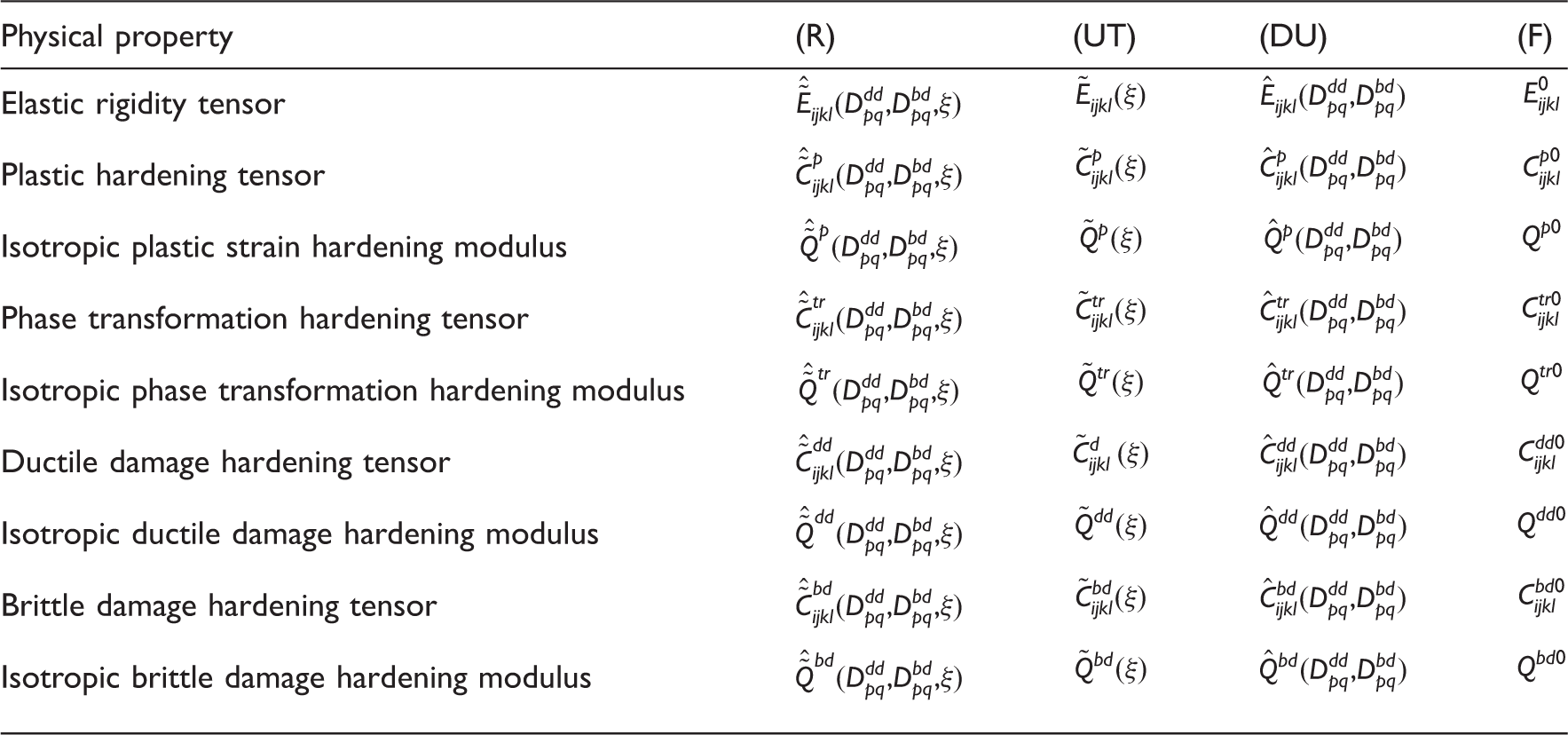
In general, different physical properties appear in equations (21) to (23) (see Table 3).

Table 3.

Physical properties associated to considered configurations.

Physical property	(R)	(UT)	(DU)	(F)
Elastic rigidity tensor	$~ \land E_{ijkl} (D_{pq}^{dd}, D_{pq}^{bd}, ξ)$	${E ~}_{ijkl} (ξ)$	${E \land}_{ijkl} (D_{pq}^{dd}, D_{pq}^{bd})$	$E_{ijkl}^{0}$
Plastic hardening tensor	$~ \land C_{ijkl}^{p} (D_{pq}^{dd}, D_{pq}^{bd}, ξ)$	${C ~}_{ijkl}^{p} (ξ)$	${C \land}_{ijkl}^{p} (D_{pq}^{dd}, D_{pq}^{bd})$	$C_{ijkl}^{p 0}$
Isotropic plastic strain hardening modulus	$~ \land Q p (D_{pq}^{dd}, D_{pq}^{bd}, ξ)$	$Q ~ p (ξ)$	$Q \land p (D_{pq}^{dd}, D_{pq}^{bd})$	$Q p 0$
Phase transformation hardening tensor	$~ \land C_{ijkl}^{tr} (D_{pq}^{dd}, D_{pq}^{bd}, ξ)$	${C ~}_{ijkl}^{tr} (ξ)$	${C \land}_{ijkl}^{tr} (D_{pq}^{dd}, D_{pq}^{bd})$	$C_{ijkl}^{tr 0}$
Isotropic phase transformation hardening modulus	$~ \land Q tr (D_{pq}^{dd}, D_{pq}^{bd}, ξ)$	$Q ~ tr (ξ)$	$Q \land tr (D_{pq}^{dd}, D_{pq}^{bd})$	$Q tr 0$
Ductile damage hardening tensor	$~ \land C_{ijkl}^{dd} (D_{pq}^{dd}, D_{pq}^{bd}, ξ)$	${C ~}_{ijkl}^{d} (ξ)$	${C \land}_{ijkl}^{dd} (D_{pq}^{dd}, D_{pq}^{bd})$	$C_{ijkl}^{dd 0}$
Isotropic ductile damage hardening modulus	$~ \land Q dd (D_{pq}^{dd}, D_{pq}^{bd}, ξ)$	$Q ~ dd (ξ)$	$Q \land dd (D_{pq}^{dd}, D_{pq}^{bd})$	$Q dd 0$
Brittle damage hardening tensor	$~ \land C_{ijkl}^{bd} (D_{pq}^{dd}, D_{pq}^{bd}, ξ)$	${C ~}_{ijkl}^{bd} (ξ)$	${C \land}_{ijkl}^{bd} (D_{pq}^{dd}, D_{pq}^{bd})$	$C_{ijkl}^{bd 0}$
Isotropic brittle damage hardening modulus	$~ \land Q bd (D_{pq}^{dd}, D_{pq}^{bd}, ξ)$	$Q ~ bd (ξ)$	$Q \land bd (D_{pq}^{dd}, D_{pq}^{bd})$	$Q bd 0$

In Table 3 it is accepted that each dissipative phenomenon may affect all physical moduli. However, it is commonly adopted that damage does not influence plastic characteristics. In the case of $γ \to α'$ phase transformation in austenitic stainless steels, the experimental evidence reveals that the elastic properties of steel remain unchanged (phase transformation does not affect elastic properties). Moreover, modeling of different dissipative phenomena may not regard for mixed hardening of all the loading functions (e.g. ductile damage development and plastic strain-induced phase transformation may be governed by plasticity within a single dissipation potential). In such cases, the number of physical moduli presented in Table 3 is substantially reduced. Therefore, in specific cases of engineering dissipative materials, the general constitutive modeling presented here is significantly simplified.

Example of application: Modeling elastic–plastic-damage two-phase material

Basic assumptions

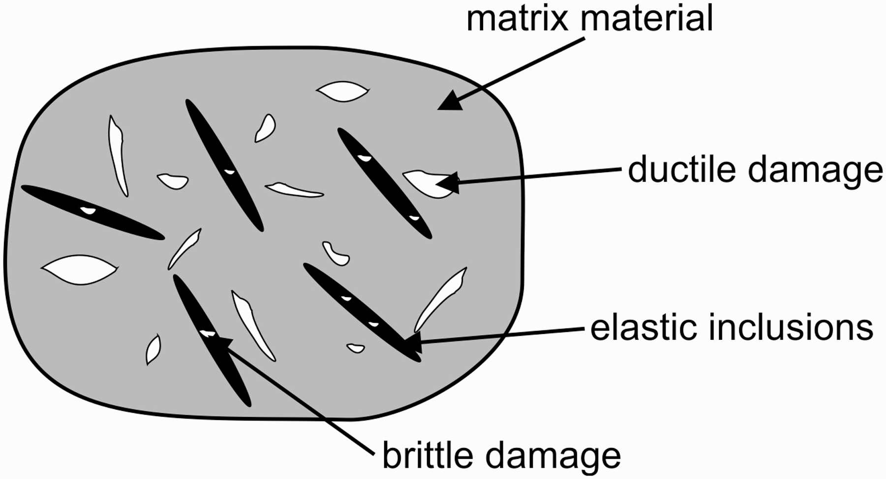
In the example, we present a macroscopic material model for simulation of three distinct dissipative phenomena taking place in a material: plastic slips, plastic strain-induced transformation from the ductile parent phase to the brittle secondary phase, and evolution of microdamage. This corresponds, for example, to austenitic stainless steel at cryogenic temperatures (cf. Egner et al., 2015a, 2015b; Ryś, 2016). The phase transformation process leads to creation of two-phase continuum, where the ductile primary phase coexists with the brittle inclusions of secondary phase (see Figure 3).

Figure 3.

Schematic representation of the elastic–plastic-damage two-phase material.

To account for the texture-induced anisotropy of the ductile matrix and damage-induced anisotropy of the brittle inclusions, the second-rank tensors $D_{ij}^{dd}$ and $D_{ij}^{bd}$ are, respectively, postulated as the measures of damage, after Egner et al. (2015a). The total material degradation in the RVE is described by the damage tensor $D_{ij}^{avg}$ , being a superposition of the ductile part $D_{ij}^{dd}$ and brittle part $D_{ij}^{bd}$ . In general, one can introduce a function $m (ξ)$ , such that $m (0) = 0$ and $m (1) = 1$ , to define a general mixture rule (cf. e.g. Hallberg et al., 2007)

D_{ij}^{avg} = (1 - m) D_{ij}^{dd} + {mD}_{ij}^{bd}

(24)

Expression $m (ξ) = ξ$ gives the simplest, linear rule of mixture

D_{ij}^{avg} = (1 - ξ) D_{ij}^{dd} + ξ D_{ij}^{bd}

(25)

In this example, it is additionally assumed that:

(A2) Both ductile damage in a matrix material and phase transformation are controlled by plasticity (within a single generalized yield function), while brittle damage evolution (in the secondary phase inclusions) is constrained by a separate damage surface. Brittle damage loading function (for simplicity) exhibits only isotropic hardening. The set of state variables (3) is therefore limited to the following elements

{V st} = {ɛ_{ij}^{E}; D_{ij}^{dd}, D_{ij}^{bd}, ξ; α_{ij}^{p}, r p, r bd}

(26)

(A3) Damage affects plastic hardening variables in the same way as elastic strains (in other words, $M_{ijkl}^{p, kin} = M_{ijkl}^{E} (D_{pq}^{dd}, D_{pq}^{bd}) = M_{ijkl}^{E} (D_{pq}^{avg}) = M_{ijkl}^{avg}$ ).

(A4) Phase transformation does not affect elastic properties of the material (cf. Mahnken et al., 2012), therefore $N_{ijkl}^{E} = I_{ijkl}$ and $P_{ijkl}^{E} = M_{ijkl}^{avg}$ .

(A5) Phase transformation affects only plastic hardening variables, therefore $h bd (ξ) = 1$ .

(A6) The phase transformation effect tensor (affecting plastic kinematic hardening variables) is a unimodular fourth-rank tensor

N_{ijpq}^{p, kin} = h kin (ξ) I_{ijpq}

(27)

According to assumptions (A3) and (A6) operator $P_{ijkl}^{p, kin}$ takes the following form

P_{ijpq}^{p, kin} (D_{pq}^{dd}, D_{pq}^{bd}, ξ) = h kin (ξ) M_{ijpq}^{avg}

(28)

Effective variables

According to assumptions (A4) and (A5), and basing on relations (14) to (16) we have

~ \land σ_{ij} = (M_{ijkl}^{avg}) - 1 σ_{kl} = {σ ~}_{ij}

(29)

~ \land X_{ij}^{p} = \frac{1}{h kin} (M_{ijkl}^{avg}) - 1 X_{kl}^{p}, ~ \land α_{ij}^{p} = h kin (M_{ijkl}^{avg}) T α_{kl}^{p}

(30)

~ \land R p = \frac{R p}{gh iso}, ~ \land r p = gh iso r p

(31)

~ \land R bd = R bd, ~ \land r bd = r bd

(32)

It is adopted here that scalar damage effect function $g (D_{ij}^{dd}, D_{ij}^{bd})$ takes the form (cf. Saanouni et al., 1994)

g (D_{ij}^{dd}, D_{ij}^{bd}) = (1 - D_{eq}^{avg}), D_{eq}^{avg} = \sqrt{D_{ij}^{avg} D_{ij}^{avg}}

(33)

and phase transformation effect functions are assumed to have the following form

(A 7) : h kin (ξ) = 1 + h_{X} ξ, h iso (ξ) = 1 + h_{R} ξ

(34)

where h_X, h_R are material parameters.

Since the phase transformation does not here affect the elastic properties of the material, $~ \land E_{ijkl} (D_{pq}^{avg}) = {E ~}_{ijkl} (D_{pq}^{avg})$ stands for the current elastic stiffness tensor affected only by damage. Adopting the total energy equivalence principle the current elastic stiffness is related to the initial stiffness of the undamaged material, $E_{ijkl}^{0}$ , by the use of the fourth-rank symmetric damage effect tensor $M_{ijkl}^{avg} (D_{pq}^{avg})$ in the following way (cf. Saanouni, 2012)

{E ~}_{ijkl} (D_{pq}^{avg}) = M_{ijpq}^{avg} E_{pqmn}^{0} M_{klmn}^{avg}

(35)

The following expression for $M_{ijkl}^{avg} (D_{pq}^{avg})$ , proposed by Cordebois and Sidoroff (1982a, 1982b), will be used here

M_{ikjl}^{avg} = \frac{1}{2} [(δ_{ik} - D_{ik}^{avg}) δ_{jl} + δ_{ik} (δ_{jl} - D_{jl}^{avg})]

(36)

Taking into account equation (24), one obtains the following decomposition of damage effect tensor

M_{ikjl}^{avg} = (1 - m) M_{ikjl}^{dd} + {mM}_{ikjl}^{bd}

(37)

where

M_{ikjl}^{dd} = \frac{1}{2} [(δ_{ik} - D_{ik}^{dd}) δ_{jl} + δ_{ik} (δ_{jl} - D_{jl}^{dd})]

(38)

and

M_{ikjl}^{bd} = \frac{1}{2} [(δ_{ik} - D_{ik}^{bd}) δ_{jl} + δ_{ik} (δ_{jl} - D_{jl}^{bd})]

(39)

State potential and state equations

The Helmholtz free energy of the material can be written as a sum of elastic (E), inelastic (I), and chemical (CH) terms

ρ ψ = ρ ψ (V st) = ρ ψ E + ρ ψ I + ρ ψ CH

(40)

In the present model, the following functions for $ρ ψ E$ and $ρ ψ I$ are adopted

ρ ψ E = \frac{1}{2} ɛ_{ij}^{E} {E ~}_{ijkl} ɛ_{kl}^{E}

(41)

ρ ψ I = ρ ψ p + ρ ψ bd = \frac{1}{2} ~ \land C_{ijkl}^{p} α_{ij}^{p} α_{kl}^{p} + \frac{1}{2} ~ \land Q p (r p) 2 + \frac{1}{2} Q \land bd (r bd) 2

(42)

The term $ρ ψ CH$ in equation (40) represents the chemically stored energy

ρ ψ CH = (1 - n) ρ ψ_{p}^{CH} + n ρ ψ_{s}^{CH}

(43)

The terms

ρ ψ_{p}^{CH} (θ)

and

ρ ψ_{s}^{CH} (θ)

are the chemical energies of the respective phases (p-primary and s-secondary), cf. for example Fischer et al. (2000), Hallberg et al. (2010), Mahnken and Schneidt (2010). Symbol

n (ξ)

denotes a function similar to

m (ξ)

in expression (24), so that

n (0) = 0

and

n (1) = 1

The chemical energies depend on the specific heat ( $c_{p}$ , $c_{s}$ ), the entropy ( $s_{p}$ , $s_{s}$ ), and temperature. The specific form of the chemical energy components, also used by Fu et al. (1993) and Hallberg et al. (2010), is taken as

ρ ψ_{i}^{CH} (θ) = - ρ s_{i} (θ - θ_{0}) + ρ c_{i} [(θ - θ_{0}) - θ \ln \frac{θ}{θ_{0}}], i = p, s

(44)

This internally stored energy is different for the two phases and it will affect the generation of heat during phase transformation, as well as the transformation itself. For inelastic strain-induced phase transformation in isothermal conditions, the chemical energy vanishes (cf. Hallberg et al., 2007).

According to hypothesis (H1) we express the state potential in the pseudo undamaged and untransformed configuration (F)

ρ ~ \land ψ E = \frac{1}{2} {ɛ ~}_{ij}^{E} E_{ijkl}^{0} {ɛ ~}_{kl}^{E}

(45)

ρ ~ \land ψ I = ρ ~ \land ψ p + ρ ψ \land bd = \frac{1}{2} C_{ijkl}^{p 0} ~ \land α_{ij}^{p} ~ \land α_{kl}^{p} + \frac{1}{2} Q p 0 (~ \land r p) 2 + \frac{1}{2} Q bd 0 (r \land bd) 2

(46)

ρ ~ \land ψ CH = ρ {ψ ~}_{primary}^{CH}

(47)

By eliminating all the reversible processes from the Clausius–Duhem inequality, the following state equation that expresses the thermodynamic force conjugated to the observable state variable is obtained

σ_{ij} = ~ \land E_{ijkl} ɛ_{kl}^{E} = ~ \land E_{ijkl} (ɛ_{kl} - ɛ_{kl}^{p} - ɛ_{kl}^{id} - ɛ_{kl}^{vol})

(48)

where

ɛ_{ij}^{p}

is the plastic strain tensor,

ɛ_{ij}^{id} = ɛ_{ij}^{idd} + ɛ_{ij}^{idb}

is the irreversible damage strain tensor, decomposed into irreversible strain tensors related, respectively, to ductile and brittle damage (cf. Abu Al-Rub and Voyiadjis, 2003; Egner, 2012), and

ɛ_{ij}^{vol} = ξ ɛ_{ij}^{trv}

, where

ɛ_{ij}^{trv} = \frac{1}{3} Δ υ δ_{ij}

, denotes the free strains describing the possible transformation-induced change of the volume, expressed in terms of the relative volume change

Δ υ

In addition, the forces conjugated to other state variables have the form

Y_{ij}^{d, avg} = - \frac{\partial (ρ ~ \land ψ)}{\partial D_{ij}^{avg}} = - \frac{\partial (ρ ~ \land ψ E)}{\partial D_{ij}^{avg}} - \frac{\partial (ρ ~ \land ψ p)}{\partial D_{ij}^{avg}} - \frac{\partial (ρ ψ ~ CH)}{\partial D_{ij}^{avg}} = Y_{ij}^{dE, avg} + Y_{ij}^{dp, avg} + Y_{ij}^{dtr, avg}

(49)

Y tr = \frac{\partial (ρ ~ \land ψ)}{\partial ξ} = \frac{\partial (ρ ~ \land ψ I)}{\partial ξ} + \frac{\partial (ρ {ψ ~}_{primary}^{CH})}{\partial ξ}

(50)

X_{ij}^{p} = \frac{\partial (ρ ~ \land ψ)}{\partial α_{ij}^{p}} = (1 + h_{C} ξ) 2 C_{rskl}^{p 0} M_{klij}^{avg} M_{rspq}^{avg} α_{pq}^{p} = ~ \land C_{ijpq}^{p} α_{pq}^{p}

(51)

R p = \frac{\partial (ρ ~ \land ψ)}{\partial r p} = (1 + h_{R} ξ) 2 (1 - D_{eq}^{avg}) 2 Q p 0 r p = ~ \land Q p r p

(52)

R bd = \frac{\partial (ρ ~ \land ψ)}{\partial r b} = Q bd 0 r bd

(53)

In the above equations, $Y_{ij}^{dE, avg}$ , $Y_{ij}^{dp, avg}$ , and $Y_{ij}^{dtr, avg}$ stand for the contributions to the thermodynamic force $Y_{ij}^{d, avg}$ from elasticity, plastic hardening, and phase transformation, respectively (cf. also Egner, 2012)

Y_{ij}^{dE, avg} = - E_{pqkl}^{0} J_{rspqij}^{avg} ɛ_{kl}^{E} ɛ_{rs}^{E}, J_{rspqij}^{avg} = \frac{\partial M_{rspq}^{avg}}{\partial D_{ij}^{avg}}

(54)

Y_{ij}^{dp, avg} = - C p 0 (1 + h_{X} ξ) 2 M_{klmn}^{avg} J_{klrsij}^{avg} α_{mn}^{p} α_{rs}^{p} + \frac{Q p 0}{D_{eq}^{avg}} (1 - D_{eq}^{avg}) (1 + h_{R} ξ) 2 (r p) 2 D_{ij}^{avg}

(55)

where

C_{ijkl}^{p 0} = C p 0 I_{ijkl}

was adopted in equation (55) for initially isotropic plasticity.

Symbol $Y tr$ denotes the thermodynamic force for phase transformation

Y tr = h_{X} (1 + h_{X} ξ) C p 0 M_{pqij}^{avg} M_{rsij}^{avg} α_{pq}^{p} α_{rs}^{p} + (1 - D_{eq}) 2 (1 + h_{R} ξ) h_{R} Q p 0 (r p) 2

(56)

and

X_{ij}^{p}

and

R p

are the plastic hardening forces, while

R bd

is the brittle damage hardening force. Equations (48) to (53) define the complete set

{J_{cf}} = {σ_{ij}; - Y_{ij}^{d, avg}, Y tr; X_{ij}^{p}, R p, R bd}

of thermodynamic forces conjugated to state variables (see Table 2).

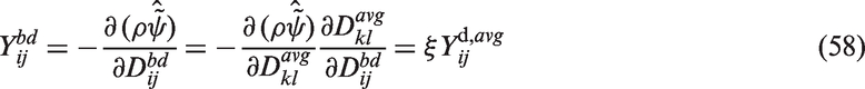
On the other hand, thermodynamic force $Y_{ij}^{d, avg}$ conjugated to damage variable $D_{ij}^{avg}$ may be decomposed into forces $Y_{ij}^{dd}$ and $Y_{ij}^{bd}$ conjugated, respectively, to damage variables $D_{ij}^{dd}$ and $D_{ij}^{bd}$ . According to equation (25) it follows that

Y_{ij}^{dd} = - \frac{\partial (ρ ~ \land ψ)}{\partial D_{ij}^{dd}} = - \frac{\partial (ρ ~ \land ψ)}{\partial D_{kl}^{avg}} \frac{\partial D_{kl}^{avg}}{\partial D_{ij}^{dd}} = (1 - ξ) Y_{ij}^{d, avg}

(57)

Y_{ij}^{bd} = - \frac{\partial (ρ ~ \land ψ)}{\partial D_{ij}^{bd}} = - \frac{\partial (ρ ~ \land ψ)}{\partial D_{kl}^{avg}} \frac{\partial D_{kl}^{avg}}{\partial D_{ij}^{bd}} = ξ Y_{ij}^{d, avg}

(58)

Evolution of state variables

We consider the following time-independent dissipative mechanisms: plastic flow, ductile damage, phase transformation, and brittle damage. We introduce for each of these mechanisms scalar-valued potential functions that are positive, null at the origin, and convex in their principal arguments.

Plastic potential $F p$ is here equal to von Mises-type yield surface plus additional terms related to isotropic and kinematic dynamic recovery (cf. Chaboche, 1999)

F p = J_{2} (σ_{ij} - X_{ij}^{p}) - σ_{y} (ξ, D_{ij}^{avg}) - R p + \frac{1}{2} \frac{b p}{Q p (ξ, D_{ij}^{avg})} (R p) 2 + \frac{3}{4} \frac{γ}{C p (ξ, D_{ij}^{avg})} X_{ij}^{p} X_{ij}^{p}

(59)

Symbol J₂ denotes the second invariant of the tensor deviator

J_{2} (σ_{ij} - X_{ij}^{p}) = \sqrt{\frac{3}{2} (s_{ij} - X_{ij}' p) (s_{ij} - X_{ij}' p)}

(60)

We adopt here the potential of ductile damage dissipation, $F dd$ , in the following form (cf. Saanouni, 2012)

F dd = \frac{2 S}{(s + 1) (1 - D_{eq}^{dd}) β} á \frac{Y dd, eq - Y_{0}^{dd}}{S} ñ (s + 1)

(61)

where S, s and β are characteristic material parameters, and

Y_{0}^{dd}

is a threshold for the norm of the thermodynamic force associated with ductile damage, below which ductile damage does not develop. Symbol

á ñ

is a Macaulay bracket to describe a ramp function.

Y dd, eq

is the norm of

Y_{ij}^{dd}

which may be defined as

Y dd, eq = \sqrt{\frac{1}{2} Y_{ij}^{dd} A_{ijkl} Y_{kl}^{dd}}

(62)

where

A_{ijkl}

is the anisotropy operator of the ductile damage evolution. The simplest case considered here is when

Y dd, eq = \sqrt{Y_{ij}^{dd} Y_{ij}^{dd}}

(63)

The phase transformation dissipation potential, $F tr$ , is expressed as a function of $Y tr$ in a simple form

F tr = f tr = AY tr - B tr

(64)

where

A (θ, σ_{ij}, {ɛ \cdot}_{ij}^{p})

, in general, is a function of temperature, stress state, and strain rate, and

B tr

is the barrier force for phase transformation (cf. Fisher et al., 2000; Mahnken and Schneidt, 2010). For rate-independent plasticity, isothermal process and small stress variations function A may be treated as a constant value (cf. Egner and Skoczeń, 2010).

According to assumption (A2) we postulate the existence of a separate brittle damage dissipation potential, $F bd$ , in the form (cf. Abu Al-Rub and Voyiadjis, 2003)

F bd = f bd + \frac{1}{2} \frac{b bd}{Q bd} (R bd) 2 = \sqrt{Y_{ij}^{bd} Y_{ij}^{bd}} - l_{bd} - R bd + \frac{1}{2} \frac{b bd}{Q bd} (R bd) 2

(65)

where damage isotropic hardening force

R bd

is expressed by equation (53). Symbol

l_{bd}

denotes the initial size (radius) of the brittle damage yield surface.

To derive the evolution equations of state variables, we will use another hypothesis (H2), after Saanouni et al. (1994):

(H2): The thermomechanical behavior of damaged and transformed medium is obtained from the same state and dissipation potentials of an undamaged and untransformed (pure elastic–plastic) medium, but expressed on the fictive configuration based on effective state variables.

Effective plastic potential $~ \land F p$ in (F) configuration is therefore here equal to von Mises-type yield surface expressed in effective variables

~ \land F p = J_{2} ({σ ~}_{ij} - ~ \land X_{ij}^{p}) - σ_{y}^{0} - ~ \land R p + \frac{1}{2} \frac{b p}{Q p 0} (~ \land R p) 2 + \frac{3}{4} \frac{γ}{C p 0} ~ \land X_{ij}^{p} ~ \land X_{ij}^{p}

(66)

where the effective variables are defined by equations (29) to (31).

The second invariant of the effective tensor deviator is expressed in the following way

J_{2} (~ \land σ_{ij} - ~ \land X_{ij}^{p}) = \sqrt{\frac{3}{2} ({s ~}_{ij} - ~ \land X_{ij}' p) ({s ~}_{ij} - ~ \land X_{ij}' p)} = \sqrt{\frac{3}{2} [(M_{ijkl}^{avg}) - 1 (s_{kl} - \frac{X_{kl}' p}{1 + h_{X} ξ})] [(M_{ijmn}^{avg}) - 1 (s_{mn} - \frac{X_{mn}' p}{1 + h_{X} ξ})]}

(67)

where

X_{kl}' p = X_{kl}^{p} - \frac{1}{3} X_{jj}^{p} δ_{kl}

is the plastic back stress deviator (in the presence of damage the incompressibility of plastic material is lost).

To derive the evolution equations of state variables (26), the normality rule (cf. Chaboche, 1997) will be used. By taking into account relation (66), the following plastic flow rule is obtained (transformational strain is here disregarded for $A = const$ in equation (64))

{ɛ \cdot}_{ij}^{I} = λ \cdot p \frac{\partial ~ \land F p}{\partial σ_{ij}} + λ \cdot dd \frac{\partial F dd}{\partial σ_{ij}} + λ \cdot bd \frac{\partial F bd}{\partial σ_{ij}} = {ɛ \cdot}_{ij}^{p} + {ɛ \cdot}_{ij}^{idd} + {ɛ \cdot}_{ij}^{ibd}

(68)

{α \cdot}_{ij}^{p} = - λ \cdot p \frac{\partial ~ \land F p}{\partial X_{ij}^{p}}

(69)

r \cdot p = - λ \cdot p \frac{\partial ~ \land F p}{\partial R p}

(70)

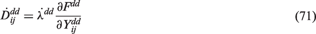
The rates of damage state variables result from the normality rule applied to the relevant potentials

{D \cdot}_{ij}^{dd} = λ \cdot dd \frac{\partial F dd}{\partial Y_{ij}^{dd}}

(71)

{D \cdot}_{ij}^{bd} = λ \cdot bd \frac{\partial F bd}{\partial Y_{ij}^{bd}} = λ \cdot bd \frac{Y_{ij}^{bd}}{\sqrt{Y_{kl}^{bd} Y_{kl}^{bd}}}

(72)

r \cdot bd = λ \cdot bd \frac{\partial F bd}{\partial R bd} =

(73)

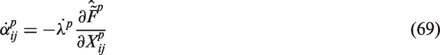
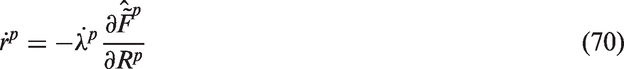
while for phase transformation we obtain

ξ \cdot = λ \cdot tr \frac{\partial F tr}{\partial Y tr}

(74)

It is further assumed here that:

(A8) ductile damage and phase transformation are governed by plasticity (cf. Egner et al., 2015a, 2015b)

λ \cdot dd = λ \cdot tr = λ \cdot p

(75)

In such simplified approach, the ductile damage and the phase transformation progress only when there is plastic flow. Similarly, beyond the ductile damage threshold there is no plasticity without a corresponding increase in ductile damage, and beyond the phase transformation threshold there is no plasticity without a corresponding increase in the secondary phase content.

By taking into account equations (74) and (75), the evolution of phase transformation variable takes the form (cf. Garion and Skoczeń, 2003)

ξ \cdot = λ \cdot p AH [(p - p_{ξ}) (ξ_{L} - ξ)]

(76)

In the above equation,

p_{ξ}

stands for the accumulated plastic strain threshold that triggers the formation of secondary phase, while

ξ_{L}

is introduced as an upper limit of a second phase content, above which the transformation rate is considered equal to 0. Symbol H denotes here the Heaviside step function.

Applying the normality rule (71) to potential function (61) the following rule governing the evolution of ductile damage is obtained

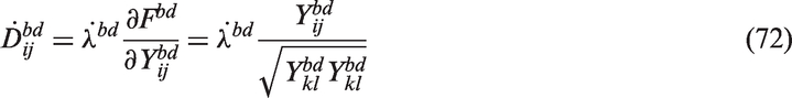
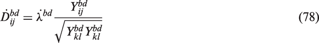
{D \cdot}_{ij}^{dd} = \frac{λ \cdot p}{(1 - D_{eq}^{dd}) β} á \frac{Y dd, eq - Y_{0}^{dd}}{S} ñ s \frac{Y_{ij}^{dd}}{Y dd, eq}

(77)

The brittle damage evolves according to the rule (72)

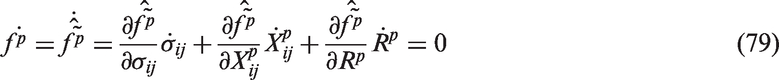
{D \cdot}_{ij}^{bd} = λ \cdot bd \frac{Y_{ij}^{bd}}{\sqrt{Y_{kl}^{bd} Y_{kl}^{bd}}}

(78)

The consistency multipliers $λ \cdot p$ and $λ \cdot bd$ are obtained from the consistency conditions expressed in the relevant configurations

f p \cdot = \land \cdot f p ~ = \frac{\partial ~ \land f p}{\partial σ_{ij}} {σ \cdot}_{ij} + \frac{\partial ~ \land f p}{\partial X_{ij}^{p}} {X \cdot}_{ij}^{p} + \frac{\partial ~ \land f p}{\partial R p} R \cdot p = 0

(79)

f \cdot bd = \frac{\partial f bd}{\partial Y_{ij}^{bd}} {Y \cdot}_{ij}^{bd} + \frac{\partial f bd}{\partial R d} R \cdot bd = 0

(80)

Fracture criterion

The simplest and most practical approach to model a mesocrack initiation is to use the critical damage criterion according to which a crack initiates when the equivalent damage $D_{eq}$ , defined as a scalar function of damage variables, reaches a critical value D_c. For a second-order damage tensor, the equivalent damage is often defined as (see equation (33)) $D_{eq} = \sqrt{D_{ij} D_{ij}}$ . Among other definitions existing in literature there are, for example, $D_{eq} = tr D$ , or $D_{eq} = max (D_{I}, D_{II}, D_{III})$ , where D_I, $D_{II}$ , $D_{III}$ are principal damage components. Fracture criterion then takes the following form

D_{eq} = D_{c}

(81)

Value of D_c is considered as a material constant that has been ascertained to be

0.2 \leq D_{c} \leq 0.8

in a number of experiments and depends on the equivalent damage variable definition (cf. Lemaitre and Desmorat, 2005; Murakami, 2012).

Parametric studies

To examine the ability of the presented model to properly predict the behavior of brittle and ductile materials, as well as the mixt ductile/brittle material, parametric studies were performed.

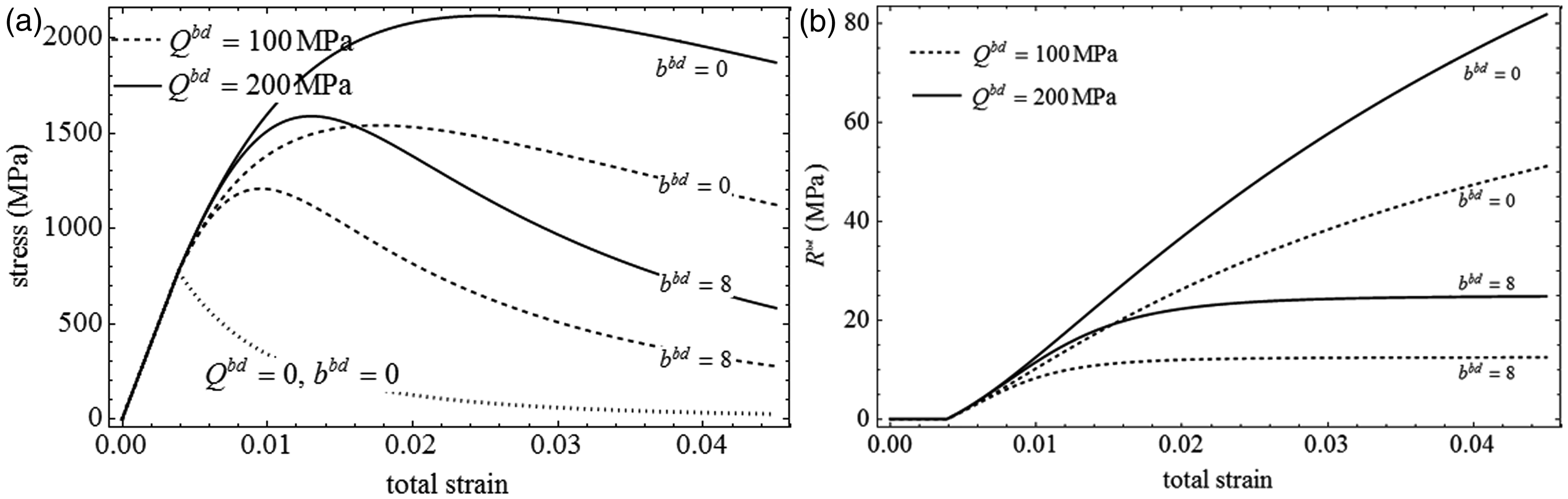
Elastic–brittle material

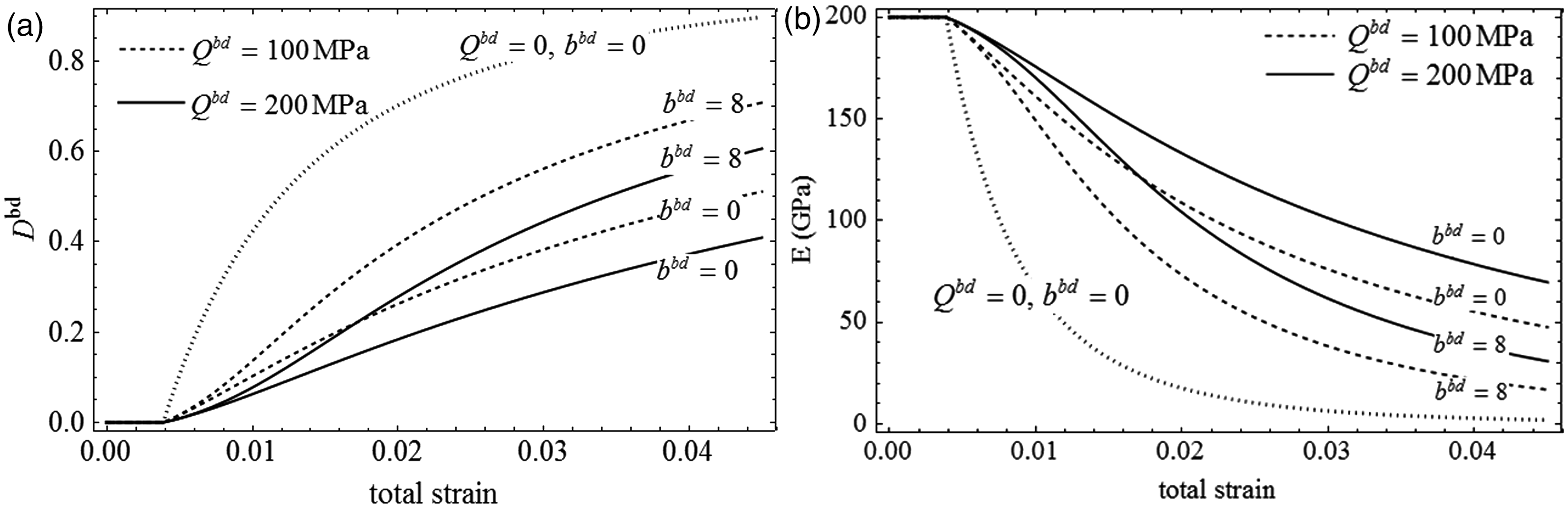
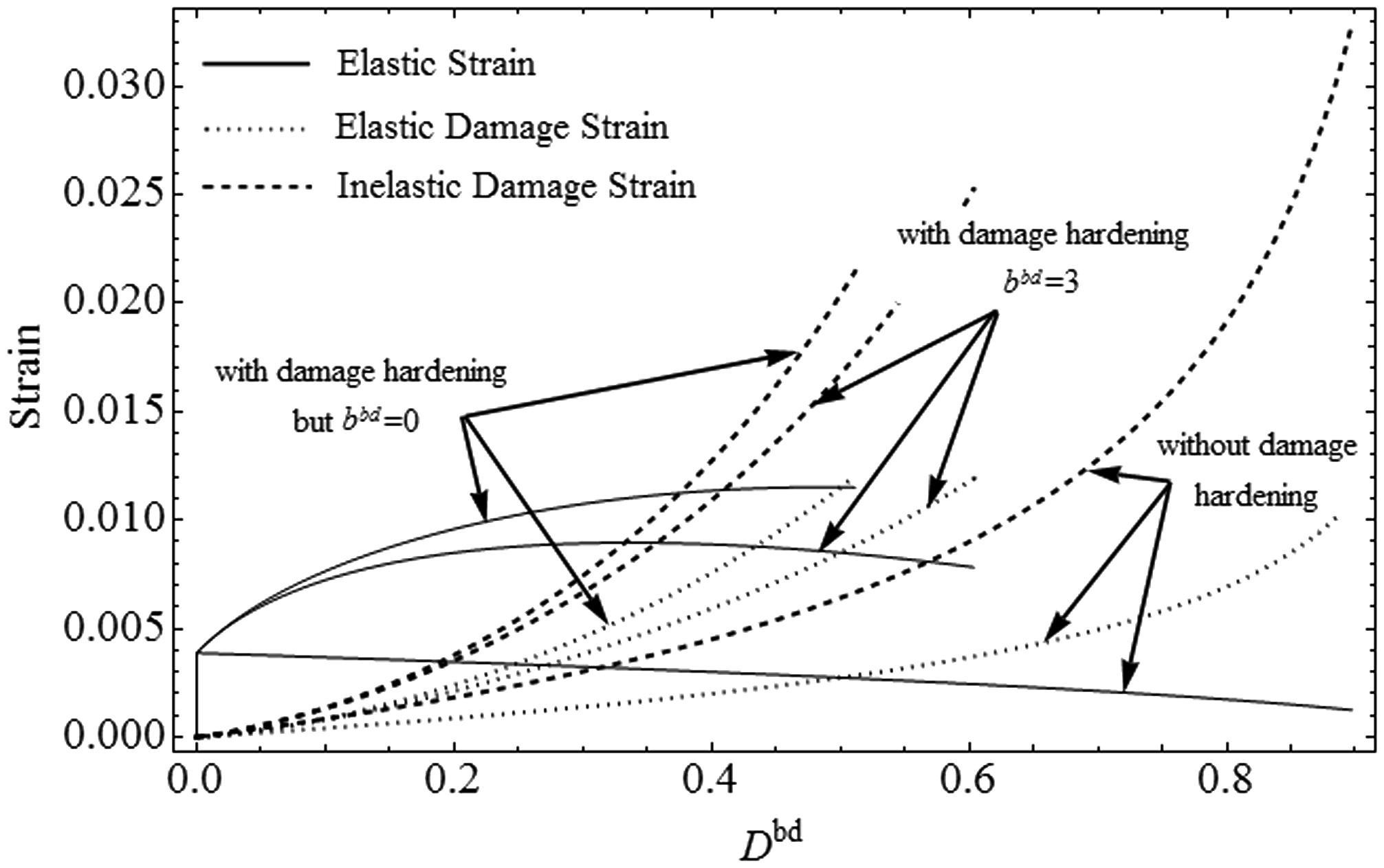
According to equation (65), three parameters were chosen that can be manipulated to change the response of the elastic–brittle material model, namely $l_{db}$ which is stress-type threshold for activating brittle damage evolution, and two parameters, $Q bd$ and $b bd$ , related to isotropic hardening of the damage surface. In Figures 4 to 6, the influence of hardening parameters $Q bd, b bd$ on the model response is presented for $l_{bd} = 3 MPa$ . Increasing the value of $Q bd$ and decreasing the value of $b bd$ implies increase in the material strength. This behavior is simply a consequence of steering the size of the damage surface which is constriction on damage evolution process and thus elastic-damage modulus degradation. It is also worth to point out that including inelastic damage strain $ɛ_{ij}^{id}$ in equation (48) has significant influence on stress–strain response, since the value of this strain is pronounced (cf. also Abu Al-Rub and Voyiadijs, 2003; see Figure 6).

Figure 4.

Influence of hardening parameters ( $Q bd, b bd$ ) on (a) stress –strain relation ( $E = 200 GPa$ ) and (b) isotropic hardening.

Figure 5.

Influence of hardening parameters ( $Q bd, b bd$ ) on (a) brittle damage evolution and (b) elastic modulus degradation.

Figure 6.

Variation of different types of strains with damage for $Q bd = 100$ MPa.

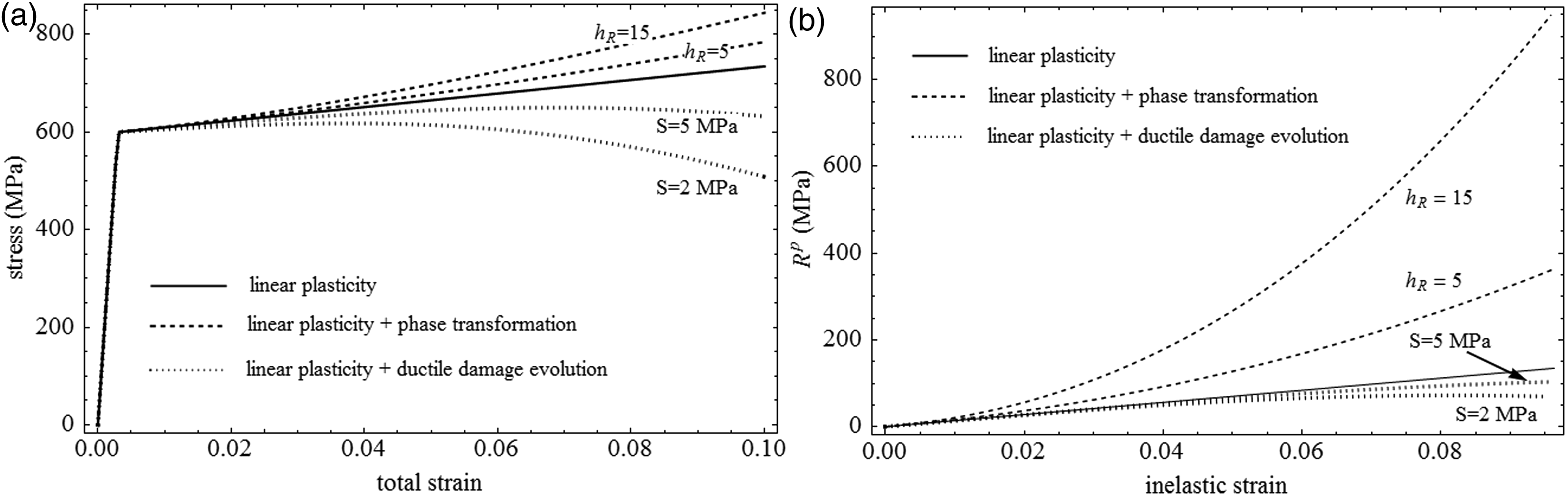
Elastic–plastic damage versus elastic–plastic phase transformation material

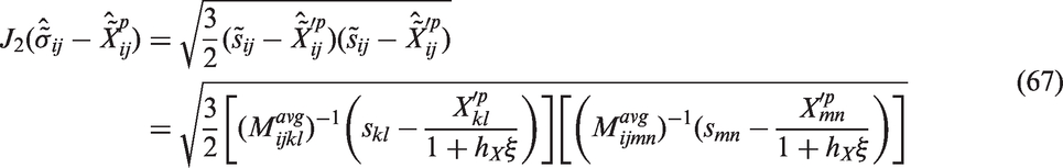
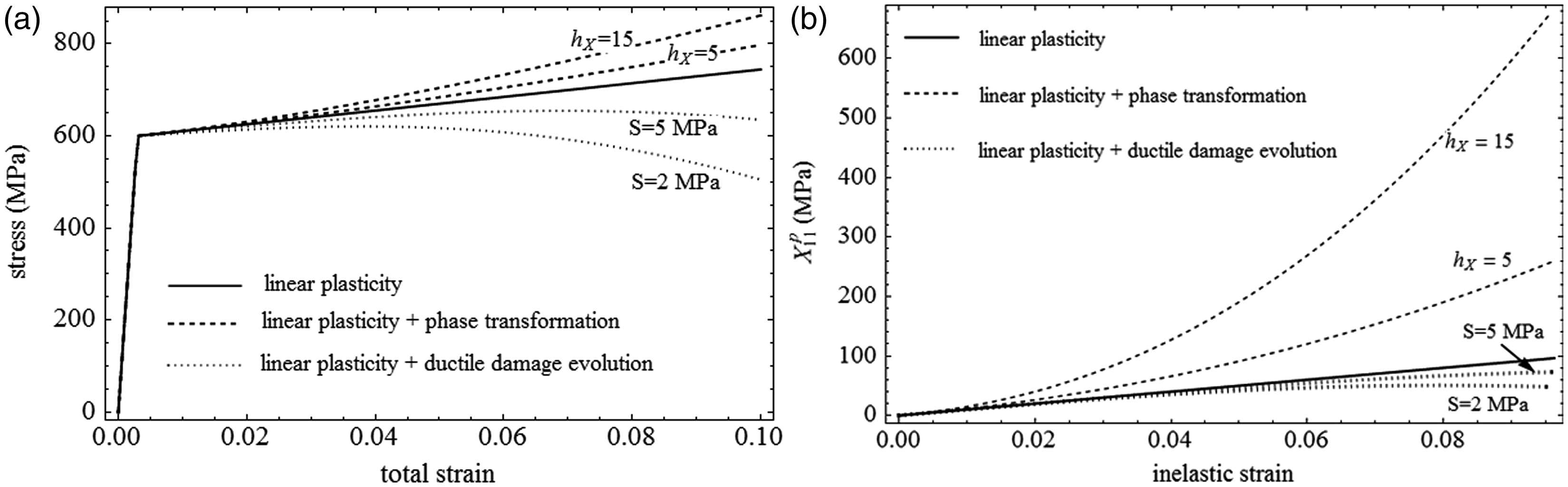
To illustrate the influence of ductile damage and phase transformation on the material response, we examine here each phenomenon separately, while brittle damage is disregarded. Thresholds for phase transformation and ductile damage were here set to $p_{ξ} = 0$ and $Y_{0}^{dd} = 0$ (see equations (76) and (77)), and the yield stress is $σ_{y} = 600 MPa$ . The phase transformation influence functions $h kin (ξ)$ and $h iso (ξ)$ (equations (30) and (31)) are monotonic increasing functions of secondary phase content to account for experimentally observed strong hardening effect due to phase transformation phenomenon. On the other hand, the damage influence tensor $M_{ijkl}^{E} (D dd)$ is a monotonic but decreasing function of damage content to enforce damage softening (see Figures 7(a) and 8(a)). Isotropic and kinematic hardening effects are here also separated (see Figures 7(b) and 8(b)). To show particular results we manipulate only three parameters: S (while $s = 1$ , and $β = 1$ , see equation (77)), h_X, and h_R (equation (34)). More detailed parametric tests of ductile damage model used here can be found in Saanouni (2012).

Figure 7.

Influence of phase transformation and ductile damage evolution on (a) stress–strain response ( $σ_{y} = 600 MPa$ ) and (b) isotropic hardening, for $Q p = 1400$ MPa (kinematic hardening disregarded).

Figure 8.

Influence of phase transformation and ductile damage evolution on (a) stress–strain response and (b) kinematic hardening, for $C p = 1000$ MPa (isotropic hardening disregarded).

Plasticity and ductile damage coupled with phase transformation

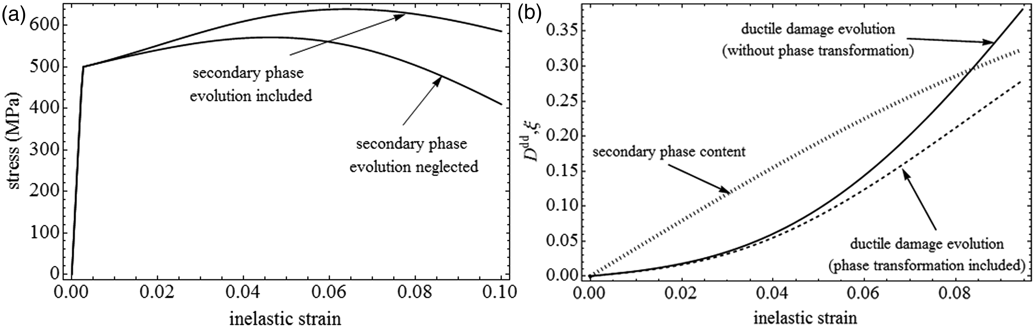
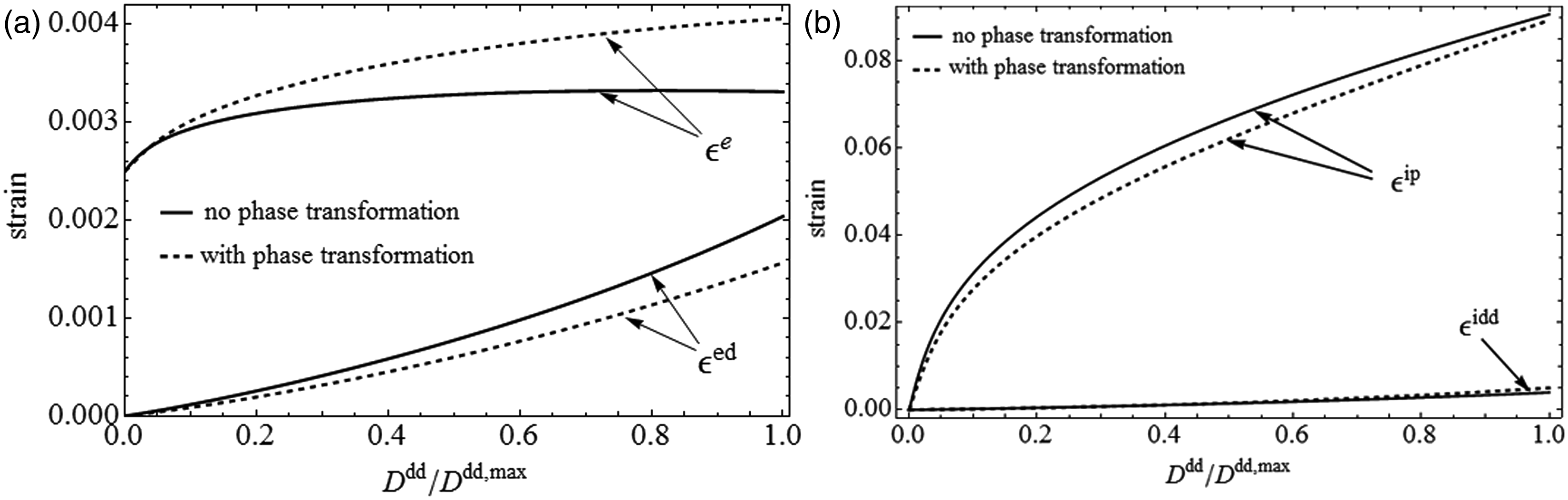
In this case, mixed linear–kinematic ( $C p 0 = 1000 MPa$ , $γ = 0$ ) and linear–isotropic ( $Q p 0 = 1400 MPa$ , $b = 0$ ) hardening laws, affected by ductile damage ( $S = 2 MPa$ , $s = 1$ , $β = 1$ ) and phase transformation ( $h_{X} = 5$ , $h_{R} = 10$ ), are used. Similarly like in previous example we can see that damage implies the material softening, whereas phase transformation results in a significant increase in strength (Figure 9(a)). The effect of phase transformation on ductile damage evolution is clearly seen (the evolution of secondary phase slows down the rate at which ductile damage evolves, Figure 9(b)). This effect was experimentally observed by Egner and Skoczeń (2010). Moreover, the model proposed in the present paper allows for mutual influence between both phenomena. Including in the model equation damage strains $ɛ_{ij}^{idd}$ (which are significant, see Figure 10) results in decreasing with damage of the phase transformation rate (Figure 9(b)).

Figure 9.

Influence of phase transformation coupled with ductile damage on (a) stress–strain response and (b) internal state variables evolution.

Figure 10.

Influence of phase transformation on the variation of different types of strains with damage.

Plasticity, mixed ductile/brittle damage, and phase transformation

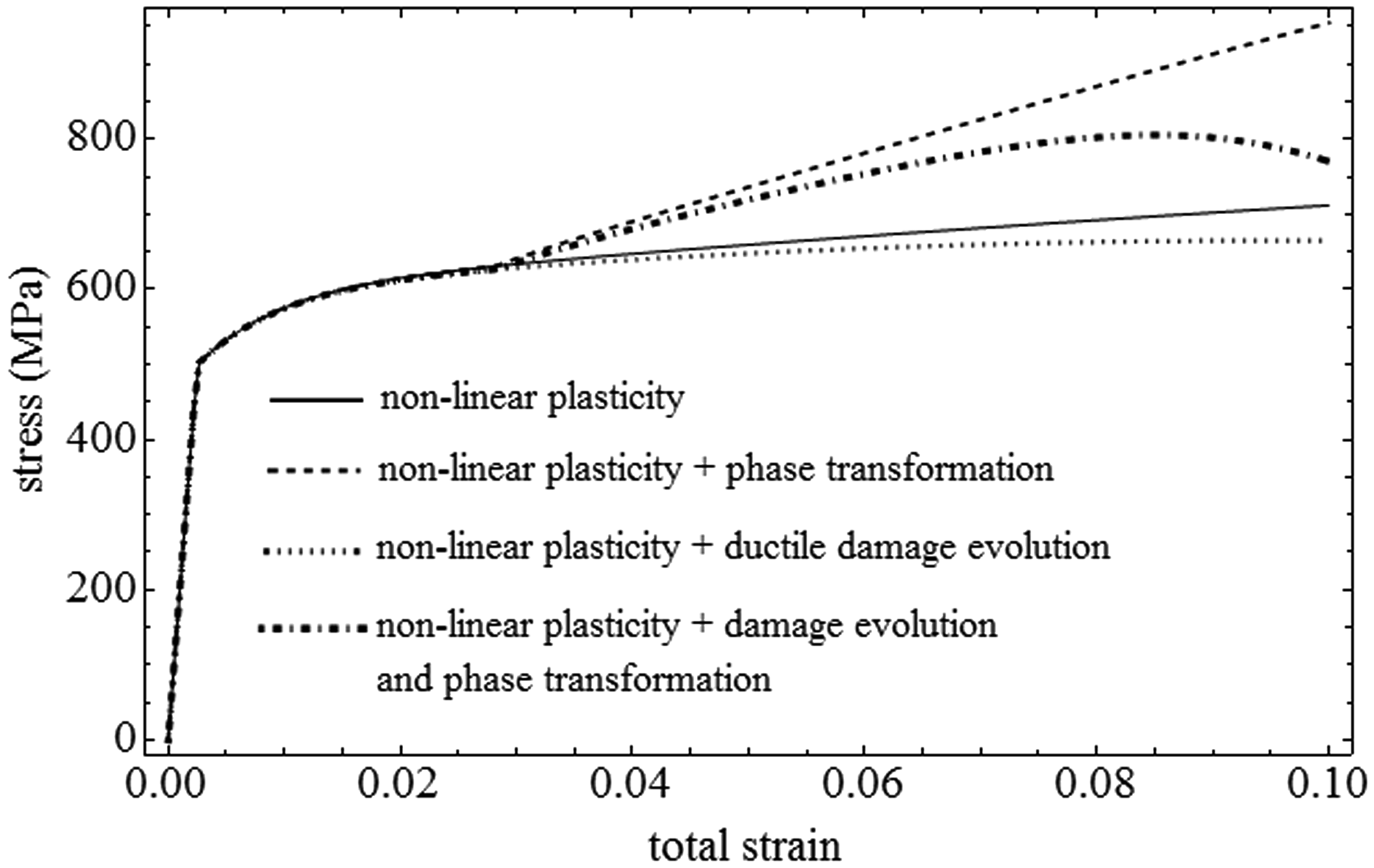
The general model of plasticity, ductile damage in matrix, phase transformation, and brittle damage in secondary phase are now considered. In Figures 11 to 16, the following cases are compared:

pure nonlinear plasticity for $C p 0 = 10, 000$ MPa, $γ = 100$ , $Q p 0 = 1400 MPa$ , $b = 4$ (solid line);

nonlinear plasticity coupled with ductile damage for $S = 10$ MPa, $s = 1$ , $β = 1$ , $Y_{0}^{dd} = 0$ (dotted line);

nonlinear plasticity coupled with phase transformation for $p_{ξ} = 0.025$ , $A = 8$ , $h_{X} = 2$ , $h_{R} = 10$ (dashed line);

plasticity, mixed ductile/brittle damage, and phase transformation, for parameters listed above and $l_{bd} = 0.3$ MPa, $Q bd = 50$ MPa, $b bd = 1$ (dashed/dotted line).

Figure 11.

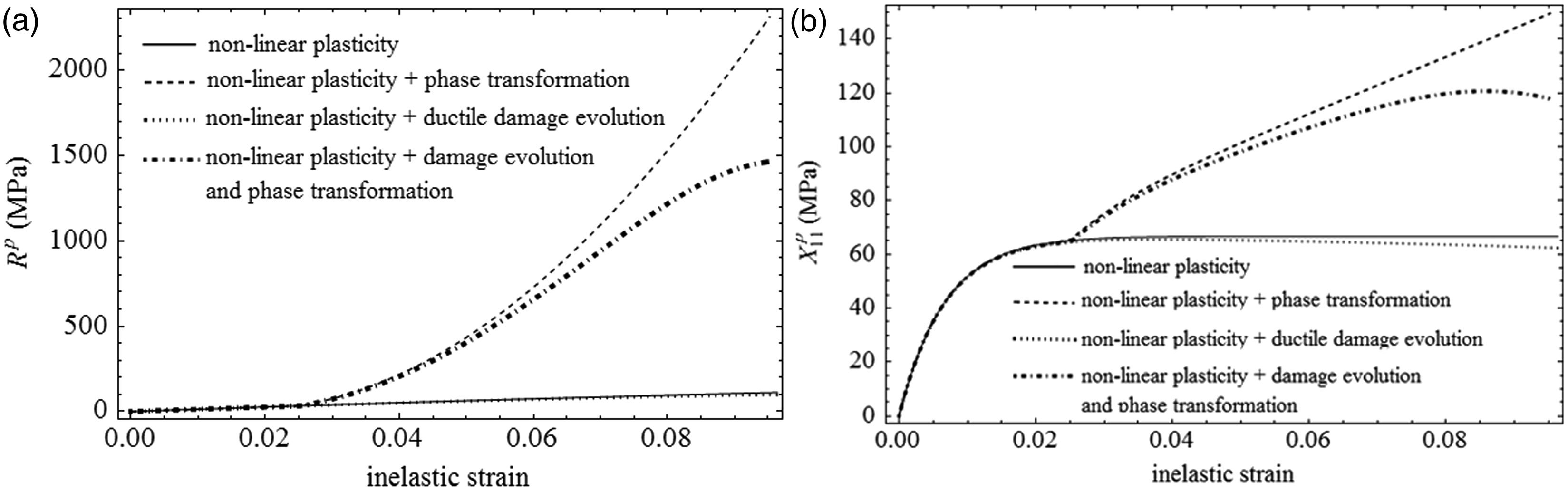
Stress–strain curves for different phenomena included.

In accordance with the physical nature of dissipative phenomena considered here (plastic strain hardening enhanced by phase transformation and damage softening), it seems that the proposed model captures all of these phenomena and couplings between them qualitatively in the proper way, what can be seen in the following figures, representing stress–strain relations (Figure 11) and thermodynamic forces related to isotropic and kinematic hardening of the yield surface (Figure 12).

Figure 12.

(a) Drag stress and (b) back stress versus inelastic strain.

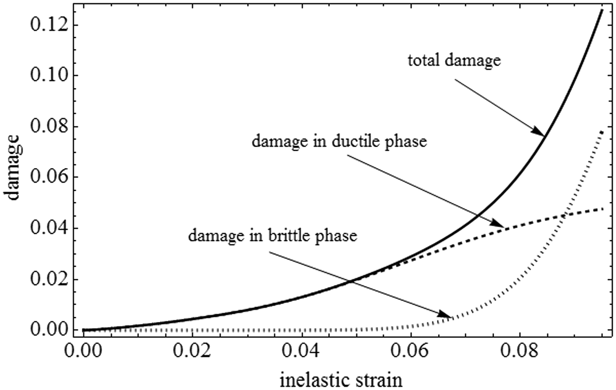
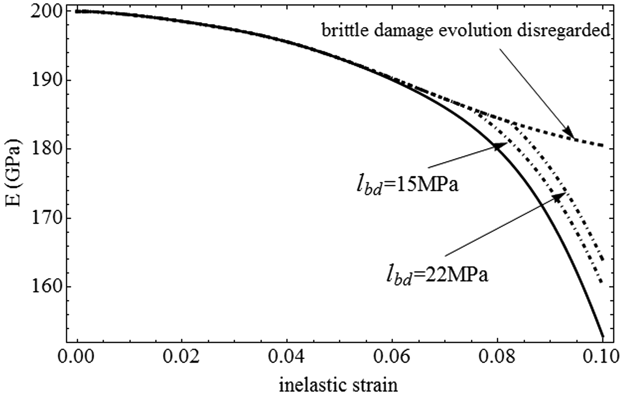
The results of the presented model for the damage variable, $D avg$ , versus inelastic strain, $ɛ_{ij}^{I}$ , are shown in Figure 13. The important result is that the use of mixture rules (25) and (37) results in the drop of the rate of the ductile damage evolution. This feature agrees with experiment (Egner and Skoczeń, 2010). In the work of Bag et al. (2001), it is noted that, in the case of dual-phase steel, substantial enhancement of the fracture toughness seems to occur for intermediate volume fractions of martensite, 30–60%, above which the enhancing effect levels off. With the use of two separate evolution laws for ductile and brittle damage, the proposed model is able to capture this physical feature. In Figure 14, we can see that if brittle damage is disregarded, the material partly recovers its initial stiffness due to the presence of the secondary phase.

Figure 13.

Damage evolution versus inelastic strain.

Figure 14.

Elastic modulus degradation.

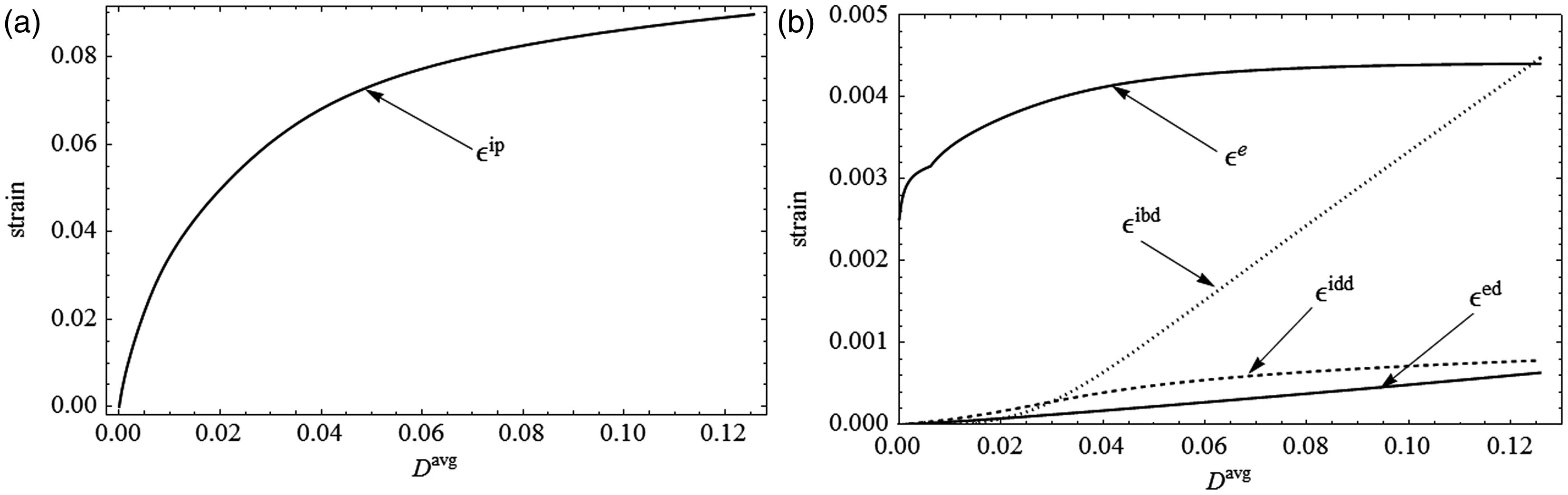
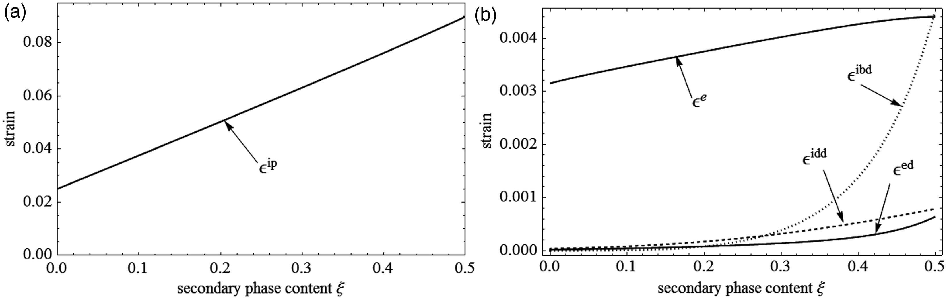
The next two figures present the development of total elastic strain $ɛ_{ij}^{E}$ components (purely elastic strain $ɛ_{ij}^{e}$ , and elastic–damage strain $ɛ_{ij}^{ed}$ ), total inelastic strain $ɛ_{ij}^{I}$ (plastic strain $ɛ_{ij}^{p}$ , and inelastic damage $ɛ_{ij}^{id}$ , further decomposed into inelastic ductile damage $ɛ_{ij}^{idd}$ , and inelastic brittle damage $ɛ_{ij}^{ibd}$ ), versus average damage $D avg$ (Figure 15) and secondary phase content (Figure 16).

Figure 15.

Variation of different types of strains with damage.

Figure 16.

Variation of different types of strains with secondary phase content.

Model behavior close to fracture

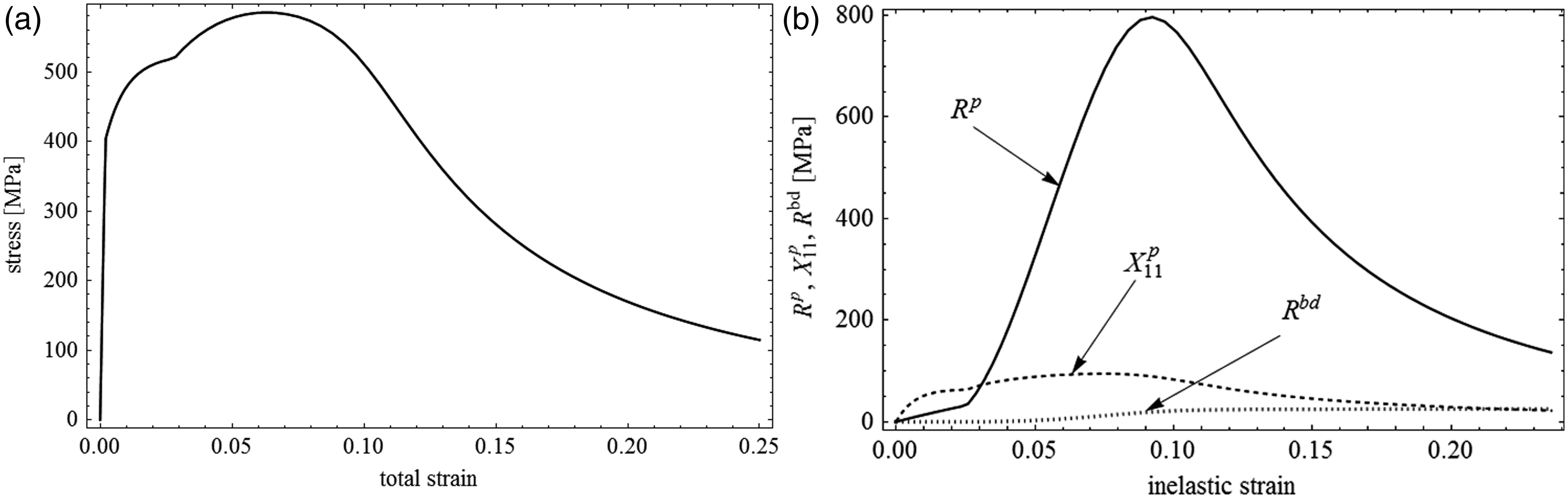
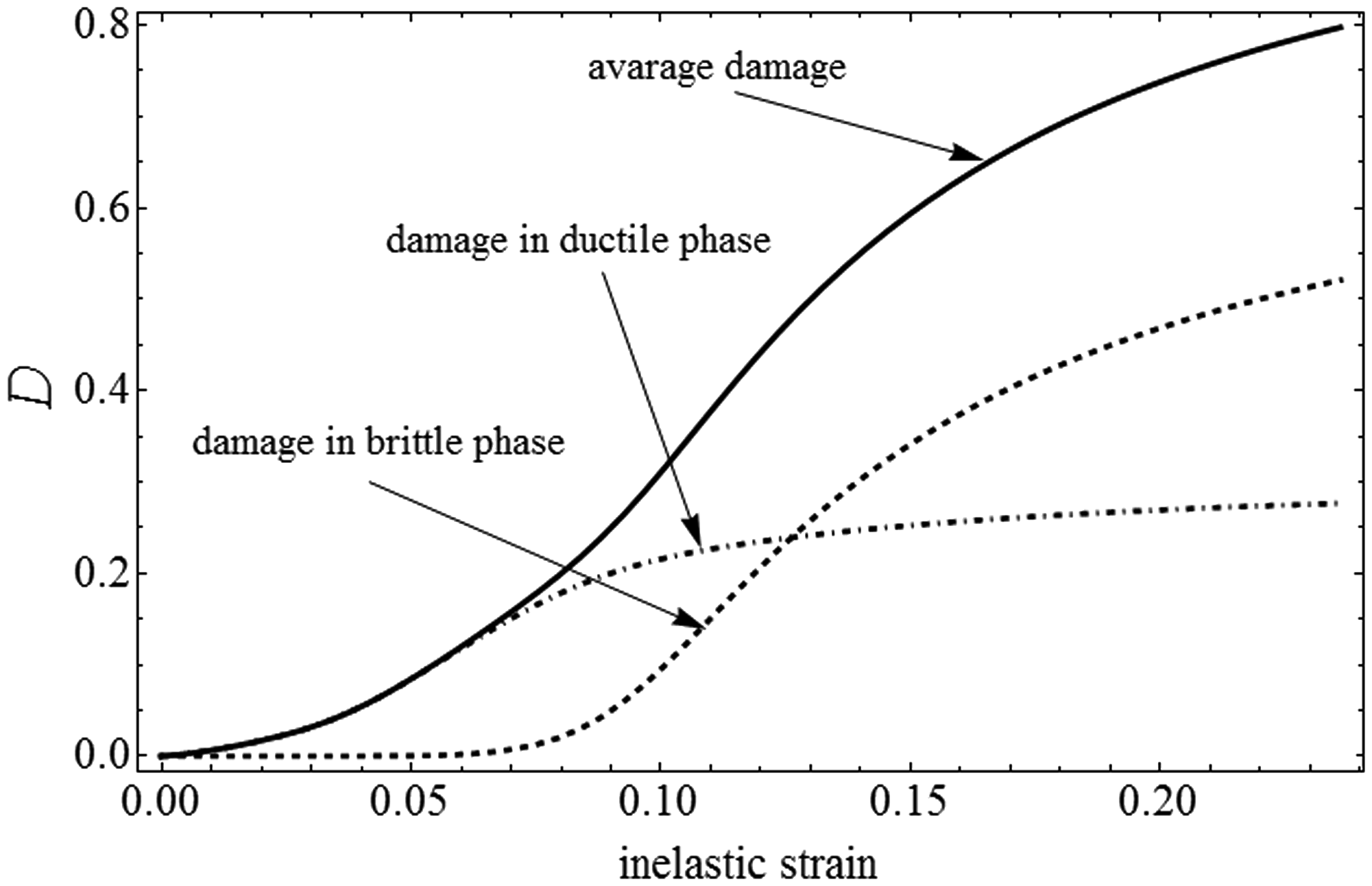
To check the model behavior near to the fracture, the simulations of uniaxial tension were performed beyond the level of small strains, until the total strain is equal to 0.25 and the average damage equal to 0.8. To enhance the influence of damage on the material behavior, the following values of material parameters related to damage evolution were applied: $S = 2$ MPa and $Q bd = 25$ MPa (the rest of parameters remains the same as in the example above). The stress–strain curve and hardening force variables (Figure 17(a) and (b)) reflect significant material softening when the level of average damage exceeds the value of 0.35. The corresponding evolution of damage components is shown in Figure 18.

Figure 17.

(a) Stress–strain curve and (b) variation of hardening force variables with inelastic strain.

Figure 18.

Damage evolution versus inelastic strain.

Conclusions

In the present paper, the approach based on the total energy equivalence hypothesis, originally developed for damaged materials, extended to modeling not only damage but also other dissipative phenomena. The material was subjected to three dissipative phenomena: plastic slips, plastic strain-induced phase transformation, and damage development, was considered as the reference material, for which the evolution of the secondary phase content gives significant rise in material strength. The approach based on the total energy equivalence allowed for different coupling effects between damage and phase transformation to appear in a natural way: secondary phase volume fraction development results in the drop of the rate of ductile damage evolution. Simultaneously, the phase transformation rate drops with the evolution of damage. On the other hand, a high volume fraction of the brittle secondary phase may provide brittle macrocracks and thus cause the material failure. These physical phenomena can be easily captured by the proposed model due to two different damage variables and different damage evolution laws used.

The analysis of dissipative phenomena presented here is limited to mechanical loads, while in general systems are subjected to the loads of different nature (mechanical, thermal, electrochemical). In such case, the traditional concept of damage appears insufficient and the generalized representation of complex damage is needed to be introduced in the framework of mechanothermodynamics (cf. Sosnovskiy and Sherbakov, 2008, 2016; Vysotskiy et al., 2011).

Footnotes

Declaration of Conflicting Interests

The author(s) declared no potential conflicts of interest with respect to the research, authorship, and/or publication of this article.

Funding

The author(s) disclosed receipt of the following financial support for the research, authorship, and/or publication of this article: This work was partially supported by the National Science Centre through the Grant No. 2015/17/N/ST8/01169.

References

Abu Al-Rub

Voyiadjis

(2003) On the coupling of anisotropic damage and plasticity models for ductile materials. International Journal of Solids and Structures 40: 2611–2643.

Bag

Ray

Dwarakadasa

(2001) Influence of martensite content and morphology on the toughness and fatigue behavior of high-martensite dual-phase steels. Metallurgical and Materials Transactions A 32: 2207–2217.

Basaran

Nie

(2004) An irreversible thermodynamics theory for damage mechanics of solids. International Journal of Damage Mechanics 13: 205–223.

Basaran

Nie

(2007) A thermodynamics based damage mechanics model for particulate composites. International Journal of Solids and Structures 44: 1099–1114.

Basaran

Yan

(1998) A thermodynamic framework for damage mechanics of solter joints. Journal of Electronics Packaging 120: 379–384.

Cauvin

Testa

(1999) Damage mechanics: Basic variables in continuum theories. International Journal of Solids and Structures 36: 747–761.

Chaboche

(1997) Thermodynamic formulation of constitutive equations and application to the viscoplasticity and viscoelasticity of metals and polymers. International Journal of Solids and Structures 34(18): 2239–2254.

Chaboche

(1999) Thermodynamically founded CDM models for creep and other conditions. In: Altenbach

Skrzypek

(eds) Creep and Damage in Materials and Structures, New York: Springer-Verlag Wien, pp. 209–278.

Chaboche

J-L

Kanouté

Roos

(2005) On the capabilities of mean-field approaches for the description of plasticity in metal matrix composites. International Journal of Plasticity 21: 1409–1434.

10.

Chaboche

J-L

Kruch

Maire

J-F

(2001) Towards a micromechanics based inelastic and damage modelling of composites. International Journal of Plasticity 17: 411–439.

11.

Cherkaoui

(2002) Transformation induced plasticity: Mechanisms and modeling. Journal of Engineering Materials and Technology 124: 55–61.

12.

Chow

(1992) An analytical and experimental study of mixed-mode ductile fracture under nonproportional loading. International Journal of Damage Mechanics 1: 191–236.

13.

Cordebois

Sidoroff

(1982a) Endommagement anisotrope en élasticité et plasticité. Journal de Mécanique Théorique et Appliquée, Numéro Spécial 45–60.

14.

Cordebois

Sidoroff

(1982b) Damage induced elastic anisotropy. In: Boehler

(ed.) Mechanical Behavior of Anisotropic Solids, The Hague: Martinus Nijhoff, pp. 761–774.

15.

Egner

(2012) On the full coupling between thermo-plasticity and thermo-damage in thermodynamic modeling of dissipative materials. International Journal of Solids and Structures 49(2): 279–288.

16.

Egner

(2015) Classification of constitutive equations for dissipative materials – general review. In: Skrzypek

Ganczarski

(eds) Mechanics of Anisotropic Materials, Switzerland: Springer International Publishing, pp. 247–295.

17.

Egner

Skoczeń

(2010) Ductile damage development in two-phase materials applied at cryogenic temperatures. International Journal of Plasticity 26: 488–506.

18.

Egner

Skoczeń

Ryś

(2015a) Constitutive and numerical modeling of coupled dissipative phenomena in 316L stainless steel at cryogenic temperatures. International Journal of Plasticity 64: 113–133.

19.

Egner

Skoczeń

Ryś

(2015b) Constitutive modeling of dissipative phenomena in austenitic metastable steels at cryogenic temperatures. In: Altenbach

Brünig

(eds) Inelastic Behavior of Materials and Structures Under Monotonic and Cyclic Loading. Advanced Structured Materials, 57. Switzerland: Springer International Publishing, pp. 35–49.

20.

Eshelby

(1957) The determination of the elastic field of an ellipsoidal inclusion, and related problems. Proceedings of the Royal Society A 376–396.

21.

Fischer

Oberaigner

Tanaka

(1997) A micromechanical approach to constitutive equations for phase changing materials. Computational Materials Science 9: 56–63.

22.

Fischer

Oberaigner

Tanaka

(1998) Transformation induced plasticity, revised and updated formulation. International Journal of Solids and Structures 35: 2209–2227.

23.

Fischer

Reisner

Werner

(2000) A new view on transformation induced plasticity (TRIP). International Journal of Plasticity 16(7–8): 723–748.

24.

Fischer

Sun

Q-P

Tanaka

(1996) Transformation-induced plasticity (TRIP). ASME Applied Mechanics Reviews 49: 317.

25.

Huo

Müller

(1993) Thermodynamics of pseudoelasticity – An analytical approach. Acta Mechanica 99: 1–19.

26.

Ganczarski

Egner

Muc

(2010) Constitutive models for analysis and design of multifunctional technological materials. In: Rustichelli

Skrzypek

(eds) Innovative Technological Materials: Structural Properties by Neutron Scattering, Synchrotron Radiation and Modeling, Heidelberg, Berlin: Germany: Springer-Verlag, pp. 179–223.

27.

Garion

Skoczeń

(2003) Combined model of strain induced phase transformation and orthotropic damage in ductile materials at cryogenic temperatures. International Journal of Damage Mechanics 12(4): 331–356.

28.

Gomez

Basaran

(2006) Damage mechanics constitutive model for Pb/Sn solder joints incorporating nonlinear kinematic hardening and rate dependent effects using a return mapping integration algorithm. Mechanics of Materials 38: 585–598.

29.

Hallberg

Hakansson

Ristinmaa

(2007) A constitutive model for the formation of martensite in austenitic steels under large strain plasticity. International Journal of Plasticity 23: 1213–1239.

30.

Hallberg

Hakansson

Ristinmaa

(2010) Thermo-mechanically coupled model of diffusionless phase transformation in austenitic steel. International Journal of Solids and Structures 47: 1580–1591.

31.

Iwamoto

(2004) Multiscale computational simulation of deformation behavior of TRIP steel with growth of martensitic particles in unit cell by asymptotic homogenization method. International Journal of Plasticity 20: 841–869.

32.

Kowalsky

Ahrens

Dinkler

(1999) Distorted yield surfaces-modelling by higher order anisotropic hardening tensors. Computational Materials Science 16: 81–88.

33.

Kruch

Chaboche

J-L

(2011) Multi-scale analysis in elasto-viscoplasticity coupled with damage. International Journal of Plasticity 27: 2026–2039.

34.

Leblond

Devaux

(1989) Mathematical modelling of transformation plasticity in steels I: Case of ideal-plastic phases. International Journal of Plasticity 5: 551–572.

35.

Lemaitre J (1971) Evaluation of dissipation and damage in metals. In: Proceeding ICM-1 Kyoto, Japan, 15–20 August 1971.

36.

Lemaitre

(1992) A Course on Damage Mechanics, Berlin and New York: Springer-Verlag.

37.

Lemaitre

Chaboche

(1978) Aspect phenomenologique de la rapture per endommagement. Journal de Méchanique Applique 2: 317–365.

38.

Lemaitre

Desmorat

(2005) Engineering Damage Mechanics, Berlin Heidelberg New York: Springer.

39.

Levitas

Ozsoy

(2009) Micromechanical modeling of stress-induced phase transformations. Part 1. Thermodynamics and kinetics of coupled interface propagation and reorientation. International Journal of Plasticity 25: 239–280.

40.

Basaran

(2009) A computational damage mechanics model for thermomigration. Mechanics of Materials 41: 271–278.

41.

Mahnken

Schneidt

(2010) A thermodynamics framework and numerical aspects for transformation-induced plasticity at large strains. Archive of Applied Mechanics 80: 229–253.

42.

Mahnken

Schneidt

Antretter

(2015) Multi-scale modeling of bainitic phase transformation in multi-variant polycrystalline low alloy steels. International Journal of Solids and Structures 54: 156–171.

43.

Mahnken

Wolff

Schneidt

(2012) Multi-phase transformations at large strains – Thermodynamic framework and simulation. International Journal of Plasticity 39: 1–26.

44.

Murakami

(2012) Continuum Damage Mechanics: A Continuum Mechanics Approach to the Analysis of Damage and Fracture, Germany: Springer Science+Business Media.

45.

Murakami

Ohno

(1981) A continuum theory of creep and creep damage. In: Ponter

ARS

Hayhurst

(eds) Creep in Structures. Third IUTAM Symposium on Creep in Structures, Berlin: Springer, pp. 422–444.

46.

Ryś

(2016) Constitutive modelling of damage evolution and martensitic transformation in 316l stainless steel. Acta Mechanica et Automatica 10: 125–133.

47.

Saanouni

(2012) Damage Mechanics in Metal Forming: Advanced Modeling and Numerical Simulation, London: ISTE/Wiley.

48.

Saanouni

Forster

Ben Hatira

(1994) On the anelastic flow with damage. International Journal of Damage Mechanics 3: 140–169.

49.

Simo

(1987) Strain- and stress-based continuum damage models. I –Formulation, II – Computational aspects. International Journal of Solids and Structures 23(7): 821–840, 841–869.

50.

Skrzypek

Kuna-Ciskal

(2003) Anisotropic elastic-brittle-damage and fracture models based on irreversible thermodynamics. In: Skrzypek

Ganczarski

(eds) Anisotropic Behaviour of Damaged Materials, Book Series: Lecture Notes in Applied and Computational Mechanics, vol. 9. Berlin Heidelberg, Berlin, Germany: Springer-Verlag, pp. 143–184.

51.

Sosnovskiy

Sherbakov

(2008) Possibility to construct mechanothermodynamics. Nauka i Innovastii 60: 24–29.

52.

Sosnovskiy

Sherbakov

(2016) Mechanothermodynamics entropy and analysis of damage state of complex systems. Entropy 18: 268.

53.

Vysotskiy

Vityaz

Sosnovskiy

(2011) Mechanothermodynamical system as the new subject of research. Mechanics of Machines, Mechanisms and Materials 15: 5–10.

54.

Wolff

Böhm

Schmidt

(2006) Modelling of steel phenomena and their interactions – An internal variable approach. Materialwissenschaft und Werkstofftechnik 37(1): 147–151.

55.

Wolff

Böhm

Suhr

(2009) Comparison of different approaches to transformation-induced plasticity in steel. Materialwissenschaften und Werkstofftechnik 40(5–6): 454–459.

56.

Yao

Basaran

(2013) Computational damage mechanics of electromigration and thermomigration. Journal of Applied Physics 114: 103708.