Creep damage and fracture of notched specimens under static and fast periodic loading

Abstract

Creep-damage processes in notched specimens subjected to static and periodic loading are studied experimentally. Subsequent simulations were carried out using Rabotnov evolution equation. In case of dynamic creep (fast periodic loading) the constitutive equations derived by use of asymptotic and averaging methods were used. Numerical results were obtained by the combination of FEM and predictor-corrector time integration scheme. Fracture process was studied using designed numerical procedure based on the elimination of the finite elements with critical values of damage parameter. The fracture times and directions of the crack propagation were determined. The qualitative difference between processes of crack propagation in cases of static and periodic loading were observed.

Keywords

Creep damage crack numerical simulation experiment

Introduction

Numerical simulation of creep deformation and fracture is an important problem, the solution to which has been found in the recent decades (Chaboche, 2002; Penny and Marriott, 1995). Both classical local and modern non-local approaches are used in order to simulate the damage accumulation, which often accompanies the process of strain growth (Almansba et al., 2012; Badreddine et al., 2010; Bažant and Jirásek, 2002; Chen et al., 2019; Hayhurst et al., 1984; Lemaitre and Chaboche, 1994; Liu et al., 2016; Paris and Saanouni, 2011; Voyiadjis et al., 2020 and many others).

Now it is generally accepted, that time to material fracture in structural element can be divided into two stages, the first one being a hidden damage accumulation up to a moment when a macroscopic defect arises, and the second one determined by the time of the macrodefect, or crack, development up to division of the element into separate parts (Penny and Marriott, 1995). Traditionally the stress-strain state is simulated separately for each stage: for the first stage we use problem formulation and solution methods from Continuum Damage Mechanics (Chaboche, 2002; Lemaitre and Chaboche, 1994) and for the second one we use those from Fracture Mechanics (Erdogan, 2000). The analysis in the first approach terminates at the moment of macrodefect’s origin, and the second one starts with the simulation of crack development without accounting for the damage distribution around it. At the same time, it is known that the separation of these two creep problems provides solutions that are essentially different from the experimental data. It is known, that the duration of stages can be commensurable (Penny and Marriott, 1995), and often crack development cannot pose any significant danger for general structural strength for a long time.

The mathematical problem formulation of general creep-damage-fracture process is well-known. It consists in creep damage analysis with gradual removal of finite elements that become ‘broken’ due to completion of the process of damage accumulation (Hayhurst et al., 1981, 1984; Ohtani, 1981; Riedel, 1989). In this area of changed geometry, the distribution of stress-strain state components and damage parameter accumulated up to the moment has to be considered as new initial conditions.

Following the development of the method for solving the problem of a crack growth under elastic-plastic deformation based on the use of the J-integral similar models were created in General Yielding Fracture Mechanics (GYFM) (Penny and Marriott, 1995). In many cases, the Finite Element Method (FEM) was used to determine the components of the stress-strain state in the structural element under creep conditions (Hayhurst et al., 1984; Ohtani, 1981). Subsequently, the approaches of Continuum Damage Mechanics were used to estimate the fracture under creep (Chaboche, 2002).

Due to the importance of the problem under consideration, new investigations devoted to the analysis of crack birth and development in physically nonlinear problems have been conducted (Brünig et al., 2015; Endo and Yanase, 2018; Jing et al., 2017; Kim and Lee, 2001; Li et al., 2019; Mengjia et al., 2016; Pandey et al., 2019; Perrin and Hayhurst, 1999; Scheider et al., 2006; Traidia et al., 2012; Wyart et al., 2007; Yatomi et al., 2003, 2008; Zhao et al., 2017). They contain experimental validation of different crack growth models as well as numerical simulation methods, which can be used in a broad range of problems. However, description of fracture processes with creep damage consideration can be considered as most complex problem due to the fact that it is boundary-initial value one.

That is why the description of creep damage accumulation and creep crack growth remained one of the most important fields of study. In this review we focus on works dealing with such problems. The effect of preliminary damage on a crack growth in a weld joint was analysed by Brünig et al. (2015). The «mechanisms based» state equation with several damage parameters was used. The area of crack initiation was determined only by damage distribution analysis without estimating its further spread.

The fracture analysis of standard specimens with cuts that model initial crack was presented in (Yatomi et al., 2003, 2008). Special preliminary procedures of mechanical processing of the specimen were done and straight grooves in it were prepared. Due to this, the straight “postulated crack path” was assumed in FEA. This approach can be used only for the analysis of crack growth, but it cannot be employed for the prediction the shape of the destroyed region in the case of structural elements of realistic geometry.

The experimental studies of the crack occurrence in a standard specimen with a notch simulating an initial crack were undertaken (Mengjia et al., 2016). Damage growth process was simulated by FEM and the time of the achieving the critical value of damage parameter was determined, which for the considered conditions determines the fracture time. An analysis of the shape of the failured material in time is not presented in this study.

A crack growth model considering creep-fatigue interaction based on continuum damage mechanics was proposed (Jing et al., 2017). Compact specimens with estimated straight crack path were analysed. FE simulation was performed with Abaqus software. The dependencies of the creep-fatigue crack rate on different crack characteristics as well as crack length on time for different loading conditions were obtained.

Creep crack growth simulations were done by Pandey et al. (2019) by use of CDM approaches and extended FEM. Compact tension and C-shaped tension specimens were analyzed. Local and nonlocal approaches were used, experimental results were compared with numerical ones. The requirements for the FE mesh are discussed.

The one of the most effective approaches consists in depletion of the finite elements in which the damage parameter reaches its critical value. Recently, this procedure was performed by elastic modulus reduction to a small value (Zhao et al., 2017). Due to the fact that this leads to the reduction in stress in the ‘broken’ elements, the real deformed and damaged states in the structural element may be significantly different. However, unlike other mechanical processes, like plastic deformation under impact, where similar procedures are realized in engineering software (for example, LS Dyna (Hallquist, 2005)), the general procedure of numerical solution for creep-damage-fracture problem currently is not implemented. It seems that there is no general procedure for removal of the element from FE mesh for arbitrary fracture direction with consideration of damage distribution. The reason can be associated with the necessity of damage redistribution simulation together with changing of calculation model, in some cases with remeshing.

Approach for FEA of the creep crack growth process taking into account the hidden damage in material is proposed by Breslavsky et al. (2018). Using the FEM Creep software (Breslavsky et al., 2017) and proposed algorithm for mesh variation with the removal of the ‘broken’ elements, the current picture of deformation and fracture is analyzed. The growing level of damage during the crack motion in each finite element was considered. Numerical fracture simulation was performed for notched specimens made of high-temperature nickel-based alloy.

The most general case of loading is the composition of constant, or static part, and varying part, which can be periodically changed. If the varying part changes with frequency greater than 1 Hz, the forced oscillations of the structures occur. Creep process under such conditions is called a dynamic creep (Lasan, 1949; Taira and Otani, 1986). Dynamic creep-damage processes are widespread in engineering structures, like jet engines, gas turbines, combustion engines, and can be characterized by essential acceleration of creep and damage growth as well as by decreasing of the times to completion of hidden damage accumulation (Lasan, 1949; Taira and Otani, 1986).

Based on the above review, the numerical simulation of the full fracture which occurs under the dynamic creep condition should be regarded as important task. The algorithm and software developed (Breslavsky et al., 2017) as well as the method for the reducing of the full dynamic creep problem into equivalent static one (Breslavskii and Morachkovskii, 1998; Breslavsky et al., 2014) can be used.

The present paper contains results of experimental and numerical investigations of the creep damage and fracture processes in statically and periodically loaded notched plane specimens. The method of dynamic creep and damage modelling is based on special constitutive equations. They were obtained by the combination of the asymptotic methods and averaging over the oscillations period. The FE algorithm of solutions with removal of the finite elements with critical damage level is used for fracture modelling. The experimental results are used for verification the employed method.

Experimental investigations of notched specimens

In this section we present the description of the experiments on creep up to fracture of standard plane and notched specimens made from duralumin D16АТ (nearest equivalent is 2024 ASTM grade) at temperature 573 K.

Description of experiments

Experimental investigations included the cases of static and fast periodic loading of standard and notched specimens. In experiments with periodic loading the stress varied according to following law:

σ = σ^{0} (1 + A \sin 2 π ϖ t), A = \frac{σ^{a}}{σ^{0}}

where σ⁰ is static stress component, σ^a is amplitude value, A is stress cycle asymmetry coefficient, ϖ = 290 Hz is the frequency of oscillations. Tests were carried with σ⁰ = 27 MPa. The values of A = 0.5 (dynamic creep) and A = 0 (static creep) were selected.

The specimen’s geometrical parameters are: operating length l = 6.6⋅10⁻² m, width b = 5⋅10⁻³ m, thickness h = 10⁻³ m. The specimens are shown in Figure 1, two of them were photographed after testing. The standard creep testing machines AIMA-5-2 were used for static loading.

Figure 1.

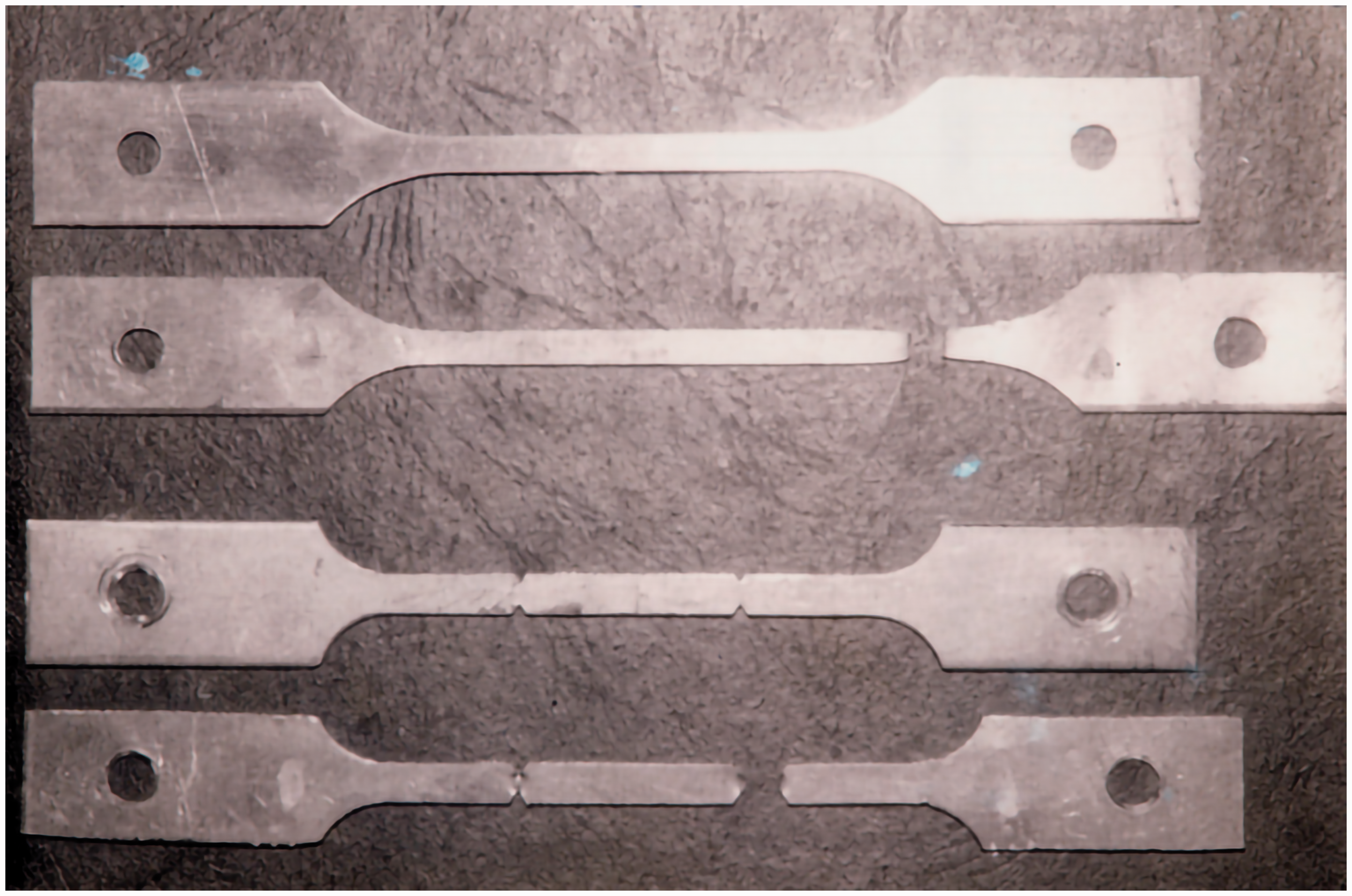
Standard and notched specimens.

Specimens were made from sheets from one delivery. For the analysis of possibility of anisotropic creep properties they were cut from sheet in different directions (along, across and in the direction with angle 45^° with reference to rolling.). For every stress level at least 3 specimens were tested. In investigations of standard specimens the creep-fracture isotropy for 573 K was previously found by Konkin and Morachkovskii (1987).

The standard testing machine AIMA-5-2 was modernized to make possible specimens testing at fast periodic loading with fixed frequency. The electrodynamic stand test bench VEDS-10A was included to the loading scheme in order to implement the periodic part of loading. The calibration of designed testing unit was done in order to determine the amount of losses in periodic loading which are associated with influence of inertia.

The way the temperature is imposed on the sample with grips is following. The sample was installed in the standard creep test machine, in which heating was conducted by the electrical oven. Three thermocouples were fastened to the top, middle and bottom parts of a sample. It was unloaded until the difference in temperature along the length of the sample does not exceed 1°–1.5 °C. After, uniformly heated specimen was loaded.

Only displacement of the specimen’s top edge is measured by standard testing machine. For smooth specimens the standard procedure of strain determination is applied, but it cannot be used for notched ones. For such specimen the measured value of displacement was used in order to compare the general levels of deformation in smooth and notched specimens. Of course, the creep strain distribution in the notch area is of great interest. The procedure of strain measurement in notch area used the measuring mesh which was plotted in notch area. The mesh variation during the creep process was measured by special comparator IZA-2, which includes microscope ОМС-6 with precision of 10⁻⁶ m.

To experimentally determine the laws of dynamic creep and fracture in case of plane stress state the studies on the notched specimens at T = 573К were performed. The geometrical parameters are identical to the parameters of standard specimens. According to standard testing conditions and recommendations (Walczak et al., 1983), four symmetric notches with angle 60^° and depth 1⋅10⁻³ m were made.

The testing protocol included the experiments on static and dynamic creep, similar to made on standard specimens. The axial loading p was varied due to the following law

p = p^{0} (1 + L \sin 2 π ϖ t), L = \frac{p^{a}}{p^{0}}

where the static axial loading component was p⁰ = 23.5 MPa, and periodic loading coefficient was L = 0.5. Three similar notched specimens were tested for each loading.

Experimental results

The results of experimental testing of static and dynamic creep on standard duralumin specimens show significant difference in creep curves. As an example, in Figure 2 the experimental values of creep strain c, % are given for static creep with A = 0 (triangle dots) and dynamic creep with A = 0.5 (round dots). Note the significant creep acceleration in the dynamic creep case.

Figure 2.

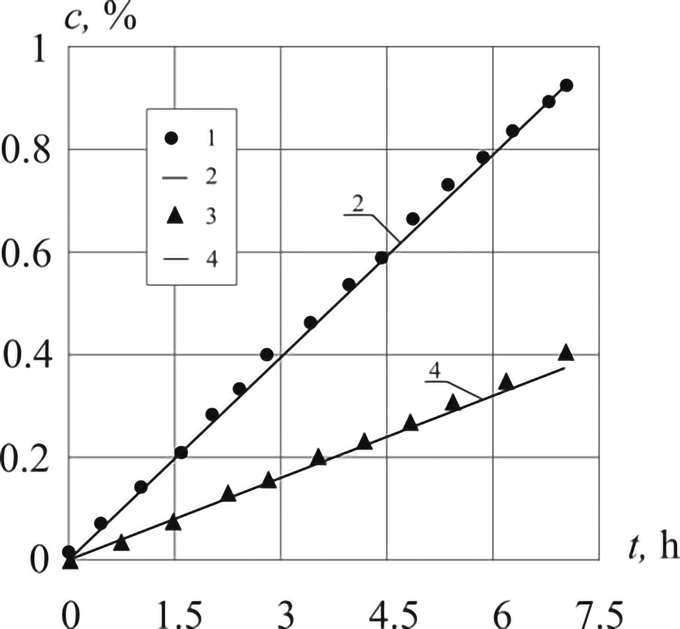
Creep curves of smooth duralumin specimens: 1, 2 – experimental and numerical results for periodic loading, 3, 4 – experimental and numerical results for static loading.

Further the experiments on notched specimens were done and analyzed.Results of averaged over three tests axial displacements of the upper sides of specimens are presented in Figure 3 by dots. The solid lines in Figures 2 and 3 represent the numerical data that are discussed in the Numerical results section.

Figure 3.

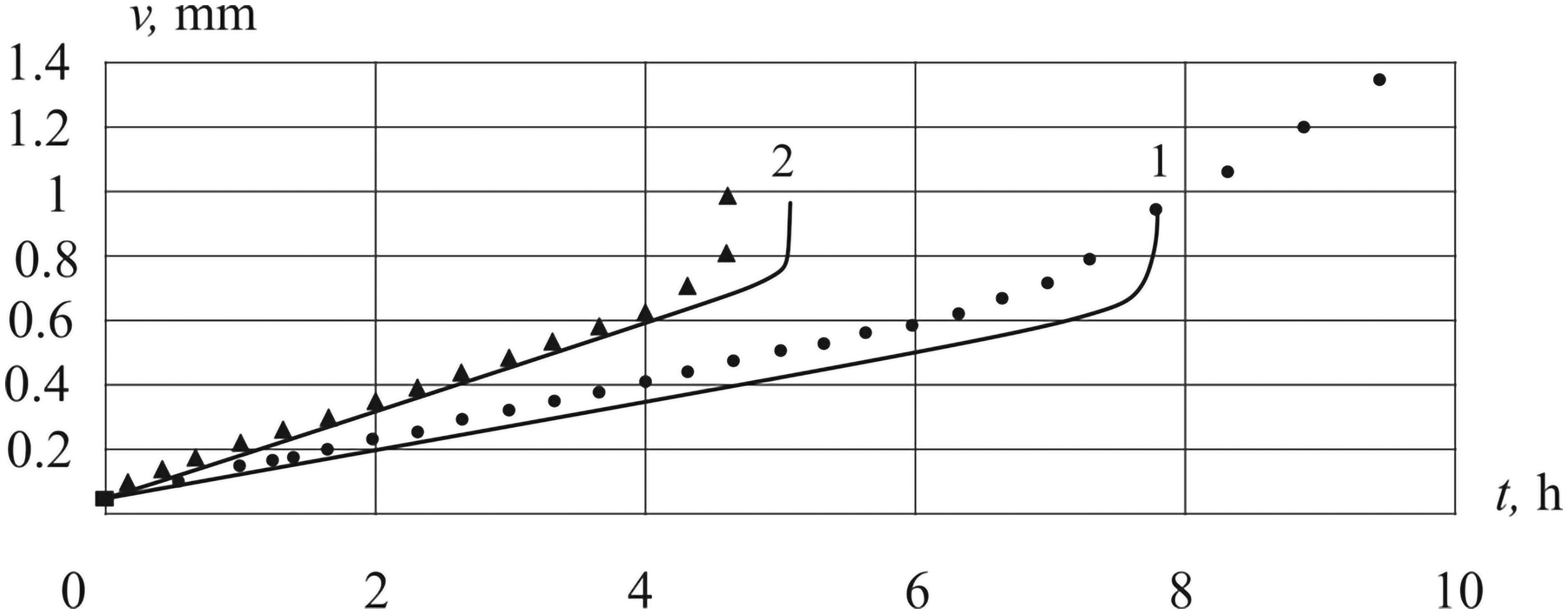
Displacements of the top side of notched specimens: 1 – static loading; 2 – periodic.

The essential creep acceleration in the case of periodic loading of standard specimens was detected both for the investigations of notched ones. The values of times to fracture differ significantly, being more than twice smaller in dynamic creep conditions (4.6 h and 9.6 h). As can be seen from Figure 3 fixed-moment value of v grows with L. For example, for t = 2 h with L = 0, v^max = 0.21 mm, and with L = 0.5 v^max = 0.36 mm, i.e. more than 1.5 times greater.

The experiments were performed until the moment of separation of notched specimens into two parts. We want to highlight the different character of tertiary creep regions in the cases of static and periodic loading. The case of dynamic creep is characterized by strongly marked transition to tertiary creep and its duration is relatively short. The static secondary creep comes to the end approximately after 6 hours of loading, and slow transition to tertiary creep with small curve’s angle begins. The values of axial displacements v in cases of dynamic and static creep, which are accumulated to the fracture moment, differ by 40%.

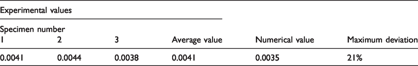
Additionally, three specimens were tested with L = 0.5 for one hour. For these specimens the measuring mesh was plotted in notch area. Creep strains were calculated based on measurements after specimen’s loading. As an example, the data for a point of mesh, which is situated near the notch contour, are presented in the Table 1, with discussion in the Numerical results section.

Table 1.

Comparison of experimental and numerical axial strain values in a notch area.

Experimental values				Numerical value	Maximum deviation
Specimen number			Average value
1	2	3	Average value
0.0041	0.0044	0.0038	0.0041	0.0035	21%

Method of numerical modelling

The mathematical problem formulation of the two-dimensional creep-damage problem for the case of static and periodic dynamic loading is presented in this section. Let us consider a 2 D area V with isotropic properties in the Cartesian coordinate system x_i (i = 1, 2). We consider small strains and displacements and homogeneous temperature field. The displacement vector with the components u_i(x, t) will be denoted by u; σ, ε are stress and strain tensors with components σ_ij = σ_ij(x_i, t) and ε_ij = ε_ij(x_i, t). All of them are functions of the coordinates point x_i (i = 1, 2) and time t.

We assume that traction p_i is applied on a part of the surface of the body S₁ as well as the displacements $u_{i} | S_{2} = {\bar{u}}_{i}$ are known on the other part of the surface S₂ (Figure 4). There are no volume forces acting on V. In the general case, the traction has the static component $p_{i}^{0}$ and the frequency-dependent component: $p_{i} = p_{i}^{0} + p_{i}^{a} \sin 2 π ϖ$ . We assume that at any moment of time the strain tensor is the sum of elastic and irreversible creep strain tensors:

ε i j = ε_{i j}^{e l} + c_{i j},

(1)

where ε^el and c are the elastic and creep strain tensors:

ε_{i j}^{e l} = ε_{i j}^{e l} (x, t)

;

c i j = c i j (x, t),

c i j (x, 0) = 0,

i, j = 1, 2.

Figure 4.

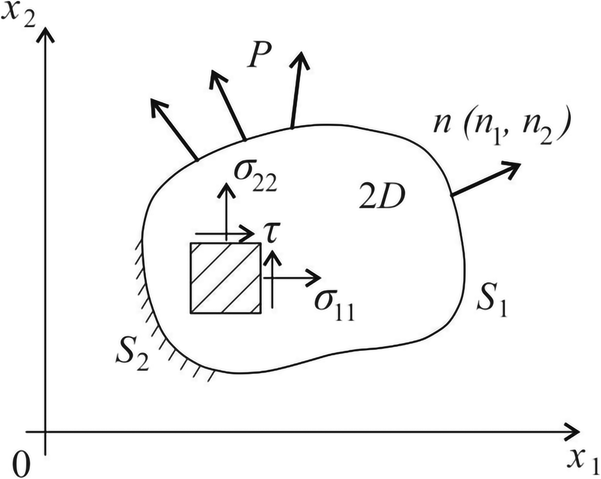
Sketch of loading and fixing of solid.

The solution procedure for the problem under consideration was formulated (Breslavskii and Morachkovskii, 1998), where the asymptotic expansion method together with the averaging over a period were applied to transform the initial system of the creep equations

σ_{i j, j} = ρ \frac{\partial^{2} u_{i}}{\partial t^{2}}, σ i j n_{j} = p_{i}, x_{i} \in S_{1};

ε_{i j} = \frac{1}{2} (u_{i, j} + u_{j, i}), x_{i} \in V; {u_{i} |}_{S_{1}} = {\bar{u}}_{i}, x_{i} \in S_{2};

(2)

σ_{i j} = C_{ijkl} (ε_{k l} - c_{k l})

into two systems. The first one coincides with the creep process in so-called ‘slow time’, in which describes the creep motion of the body neglecting small strain variations over the period of oscillations

T = \frac{1}{ϖ}

\begin{array}{l} σ_{i j, j} = 0, x_{i} \in V; σ i j n_{j} = p_{i}, x_{i} \in S_{1}; \\ ε_{i j} = \frac{1}{2} (u_{i, j} + u_{j, i}), x_{i} \in V; {u_{i} |}_{S_{1}} = {\bar{u}}_{i}, x_{i} \in S_{2}; \\ σ_{i j} = C_{ijkl} (ε_{k l} - c_{k l}) \end{array}

(3)

where n is the unit vector of the outer normal to the surface S₂ of the body, n={n_i, i = 1,2}; C_ijkl are the components of elastic constants tensor, ρ is the mass density.

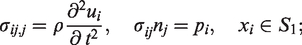
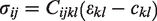
In equation (2) at every moment of time the creep strains are determined by the creep-damage constitutive equations of the dynamic creep phenomenon, which were obtained from Norton law and Kachanov-Rabotnov damage equation with Rabotnov-Shesterikov modification (Lokoshchenko and Shesterikov, 1980) by use of the same asymptotic and averaging procedures (Breslavskii and Morachkovskii, 1998; Breslavsky et al., 2014):

{\dot{c}}_{i j} = B (1 + H (A)) \frac{{(σ_{i})}^{n}}{{(1 - ω^{r})}^{n}}, s_{i j}, \dot{ω} = D (1 + K (A)) \frac{{(σ_{e q})}^{n}}{{(1 - ω^{r})}^{n}}, ω (x, t_{0}) = ω_{0}, ω (x, t_{*}) = ω_{*}

(4)

where

$σ_{i} = \sqrt{\frac{3}{2} s_{i j} s_{i j}}$ is von Mises equivalent stress, $σ_{e q} = α \cdot Sup (σ_{1}, σ_{2}, σ_{3}) + (1 - α) σ_{i}$ is equivalent stress for damage description (Lemaitre and Chaboche, 1994) σ_k (k = 1,2,3) are principal stresses, α is the constant, s is the stress deviator.

H (A) = \int_{0}^{1} {(1 + A \sin (2 π ξ))}^{n} d ξ - 1, K (A) = \int_{0}^{1} {(1 + A \sin (2 π ξ))}^{n} d ξ - 1

are the influence functions which describe the dynamic creep and damage acceleration.

A = \frac{σ_{i}^{a}}{σ_{i}}

is the stress cycle asymmetry coefficient, A < 1 (Taira and Otani, 1986). The static creep is described by A = 0. The function ω=ω(x, t) is the scalar damage parameter, B, n, D, r are the material constants.

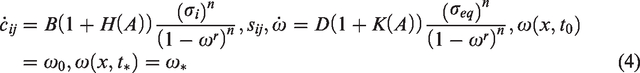
The superscript a in expression for A indicates that this von Mises stress is determined by the amplitude stress components. To find them in every point the second system of differential equations, which describes the forced oscillations in the frequency region far from resonance, has to be solved (Breslavskii and Morachkovskii, 1998):

\begin{array}{l} σ_{i j, j}^{a} = - ρ ϖ^{2} u_{i}^{a}, x_{i} \in V; \\ σ_{i j}^{a} n_{j} = p_{i}^{a}, x_{i} \in S_{1}; \\ ε_{i j}^{a} = \frac{1}{2} (u^{a} i, j + u^{a} j, i) = C_{ijmn} σ_{m n}^{a} x_{i} \in V; \\ u_{i}^{a} (0) = 0 x_{i}, \in S_{2} . \end{array}

(5)

When the development of internal damage in the solid’s volume ends, the macrodefect arises. In this case, the solid volume V decreases by the value of ΔV, and its boundary line also changes by the value of ΔS. Also, analyzing the possible fracture situations (Penny and Marriott, 1995), we can suggest, that in many cases it is probable that the parts of the boundary S₁ and S₂, where the boundary conditions in stresses and displacements are set, will also change by the values ΔS₁ and ΔS₂ due to possible fracture of fixed and loaded boundaries

S_{1} = S_{1} + Δ S_{1}; S_{2} = S_{2} + Δ S_{2}

(6)

We can say that for moment of time t_* the next relation takes place:

V = V + Δ V; S = S + Δ S

(7)

For boundary points in equations (6) and (7) operations are written in the algebraic sense, i.e. the increments of S can be positive or negative.

By the end of the period of hidden damage accumulation t_*, each point of the solid is characterized by the values of the stress-strain state components: stresses $σ_{i j}^{*}$ , total strains $ε_{i j}^{*}$ , creep strains $c_{i j}^{*}$ , displacements $u_{i}^{*}$ and damage parameter $ω *$ .

So, boundary-initial value problem (2) is formulated with following initial conditions:

u_{i} (x_{i}, t_{*}) = u_{i}^{*} (x_{i}); c_{i j} (x_{i}, t_{*}) = c_{i j}^{*} (x_{i}); ε_{i j} (x_{i}, t_{*}) = ε_{i j}^{*} (x_{i}); σ_{i j} (x_{i}, t_{*}) = σ_{i j}^{*} (x_{i}); ω (x_{i}, t_{*}) = ω^{*} (x_{i})

(8)

This problem’s solution has to be continued up to the moment of finishing of the process of hidden damage accumulation in a new point. Then the algorithm for rearranging the boundary and initial conditions is repeated and new boundary-initial value problem is formulated.

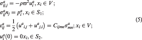
The boundary-initial value problem is solved by FEM in combination with the third-order predictor-corrector method for time integration. We used the software complex FEM CREEP (Breslavsky et al., 2017), the vector-matrix formulation of the problem for finite element is presented in the following form:

\begin{array}{l} (\int V {[B]}^{T} [C] [B] d V) {{\dot{u}}^{γ}} = \int_{V} {[B]}^{T} [C] {{\dot{c}}^{β}} d V + \int_{S_{1}} {[N_{2 d}]}^{T} {\dot{p}} d S, \\ {{\dot{σ}}^{β}} = [C] ({{\dot{ε}}^{β}} - {{\dot{c}}^{β}}), \\ {{\dot{ε}}^{β}} = [B] {{\dot{u}}^{γ}} \end{array}

(9)

where γ indicates the number of node as well as β indicates the number of finite element;

[B] is the matrix differentiation operator;

[C] is the matrix of elastic characteristics of the material;

{u^γ} is the vector of nodal displacements;

{σ^β}, {ε^β}, {с^β} are the vectors of stresses and elastic and creep strains in the element;

[N_2d] is the matrix, which expresses by means of shape functions the value of any displacement of the element through the node.

The integral in parentheses on the left-hand side of the first equation (9) corresponds to the stiffness matrix of the element [K^β].

After the procedure of assembling the system of finite elements, the following system of differential equations is obtained:

[K] {\dot{u}} = {\dot{F}} + {{\dot{F}}^{c}}

(10)

where [K] is the system’s stiffness matrix;

{u} is the global vector of nodal displacements;

{F} is the vector of nodal loads from traction;

{F^с} is the vector of nodal forces resulting from creep strains.

For time integration, at each step the stress and strain vectors components and damage parameters in finite elements as well as nodal displacements are determined numerically.

The system (5) describing the forced oscillations is derived to the FE system of algebraic equations with reference to vector on nodal amplitude displacements {u^a} and nodal amplitude forces {F^a}.

[K - Ω^{2} M] {u^{a}} = {F^{a}}

(11)

where [M] is the mass matrix of the system. Amplitude displacements {u^a} found from this system’s solution are used to determine stress cycle asymmetry coefficient A in each element. A varies in time due to processes of stress redistribution. In the absence of forced oscillations (A = 0) we reduce to the classical creep-damage problem.

In the classical method of the creep-damage problem solution the moment of the achieving the damage parameter ω its critical value ω _* is considered as the ending point of long-term strength analysis. This moment of time determines the appearance of a macrodefect at this point.

The presented algorithm allows to do the full analysis of the fracture process. It consists of subsequent solution of creep-damage problems by use of the system of equations (2) and (3) but with changed geometry of the object as well as with possible changing of boundary conditions due to removing ‘broken’ finite elements. The new initial conditions contain the current values of the stress-strain state components as well as the damage parameter at all points. It is postulated, that macrocrack with length equal to characteristic dimension of ‘broken’ FE length l is born after first creep-damage problem solution.

The algorithm iterations has to be continued until the fracture criterion which assumed for the given problem is satisfied. For us, the criterion is the fracture region (macrocrack) achieving a certain critical length l_*. The details of the creep-damage-fracture algorithm for plane stress state can be found in [22], here we present a flowchart as a summary (Figure 5).

Figure 5.

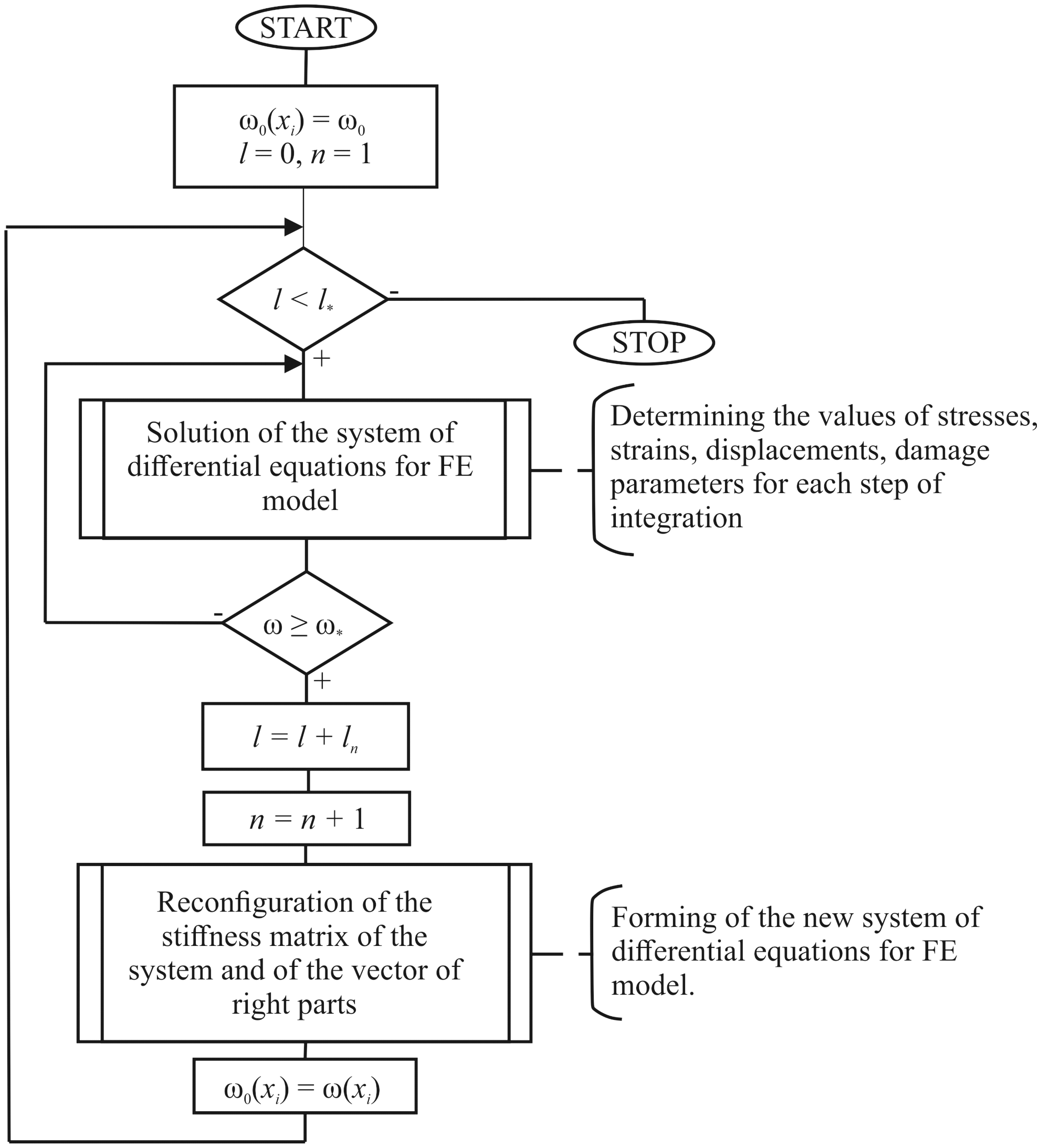
Flowchart of the FE creep-damage-fracture algorithm (Breslavsky et al., 2018).

The triangular element with three nodes is implemented in developed software (Breslavsky et al., 2017). This element has several advantages. First, the linear approximation of displacements leads to constant stress values in each element, as well as the value of damage parameter ω. This allows removing the entire finite element from the mesh at the moment when damage parameter reaches its critical value ω_*. In more complex finite elements the value of stress and therefore damage parameter are different in different points. Therefore the procedure of element’s elimination in failure analysis has to be more complex due to the necessity of additional approximations of damage distribution. This leads to growth of the dimension of the system of equations. The second reason is the possibility of a simple description of the model shape as well as of macrodefect shape in the process of failure analysis.

One of the key feature of the proposed approach is the following. After the start of the fracture process we can assume that we have new stress concentration in area where finite element(s) was removed. In order to avoid remeshing we have to use the mesh that will be capable of simulating the area with new configuration. That is why the mesh is regular and the FE dimensions in it were determined by numerical experiments. The detailed description of used method, algorithms and software can be found in Breslavsky et al. (2017, 2018).

Numerical results

The equation (4) which were used for description of static and dynamic creep of the duralumin standard specimens tested experimentally. Figure 2 contains the comparison of experimental (dots) and numerical results obtained by solving equation (4) (solid lines: dynamic creep (curve 2) and static creep (curve 4). The difference does not exceed 3–4%. Therefore, such result allows us to use the creep-damage law (4) for the case of complex stress state.

Further, we present the FEA results for creep and fracture of notched specimens. The calculation scheme of plane stress was used. For studied duralumin the damage equivalent stress σ_eq is equal to the von Mises stress σ_i: α = 0 and σ_eq=σ_i (Konkin and Morachkovskii, 1987).

The experimental data of static and dynamic creep for L = 0.5 in notched specimens presented in the Experimental investigations of notched specimens section were used for validation of the method and algorithm of creep-damage-fracture analysis. Due to symmetry of notches, two FE models were applied. The model 1 presents one-half of full length of the specimen taking into account the axial symmetry with respect to the direction of tension. For this scheme, the creep-damage problem was solved up to the moment when the critical value of damage parameter in notch tip is reached.

Let us take a closer look at the deformed state of notched specimens. Numerically obtained by use of the model 1 maximum value of axial displacement v^max is presented in Figure 3 by solid lines. As we see from this figure, the numerical data describe the results of deformation (dots) qualitatively correct.The results of quantitative estimation can be considered as acceptable too: the differences between maximum and minimum values of v^max were for creep displacements is not greater 30%, for elongations at the fracture moment is not greater than 25%.

The obtained numerical data of strain state in notched specimens in dynamic creep conditions were compared with experimental values, which were additionally obtained by measurements of meshes in notch area at t = 1h. The axial strains c_у for each of the three tested specimens as well as average and numerical values are presented in a Table 1.

Comparison between experimental and numerical axial strain values in the same points of FE model shows acceptable difference of 21%. So, it can be considered as additional validation of used 2 D method and FE software for the plane stress case.

Further, due to symmetry with respect to pairs of notches, the model 2 of one-quarter of specimen was used (Figure 6). The length of FE model in axial direction was truncated due to results of series of numerical solutions, in which the equivalent traction influence in axial direction was controlled. For this model, after the numerical experiments, the mesh with 4276 elements was selected.

Figure 6.

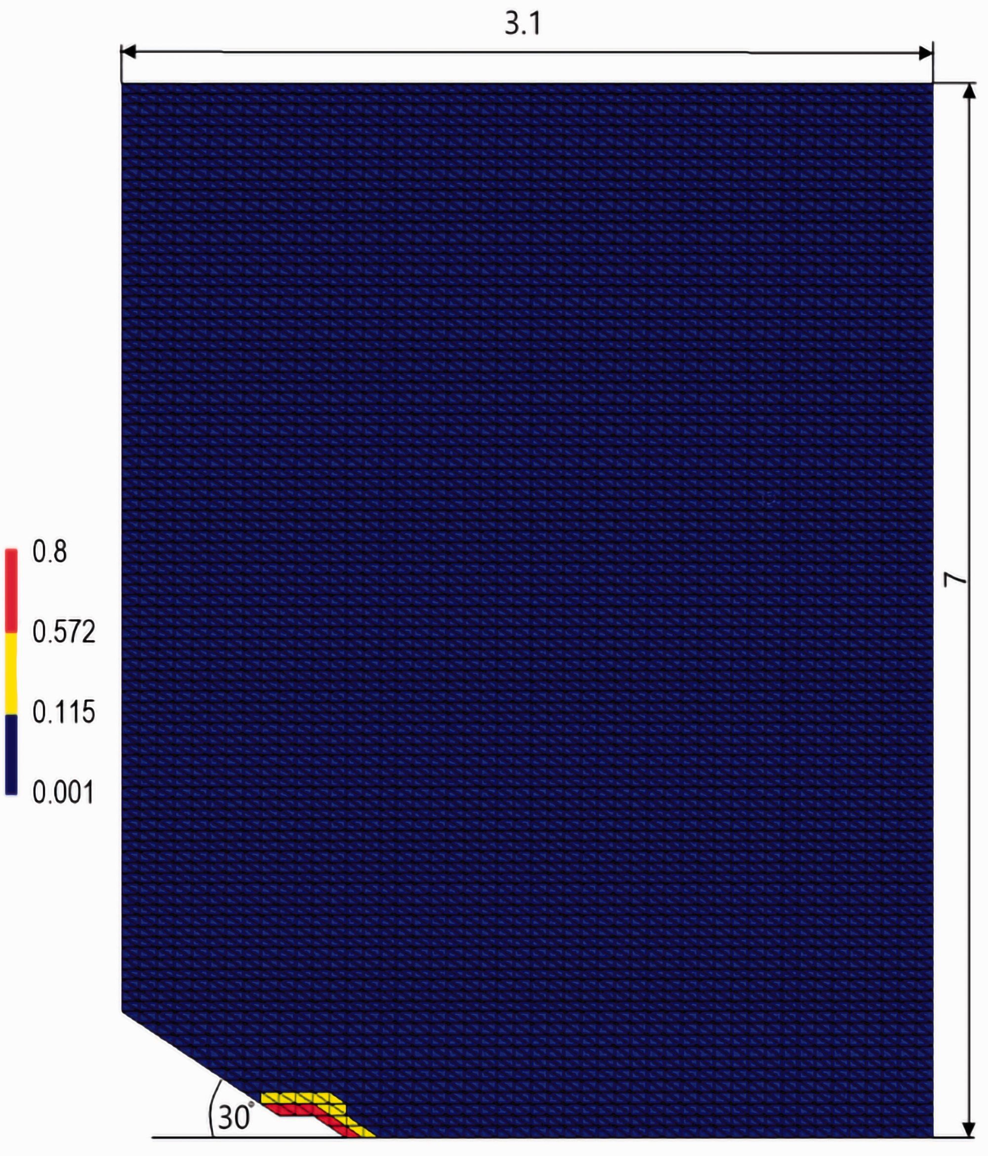
FE model of the part of the notched specimen (dimensions in mm). Mesh with 9287 elements.

One of the goals of the present study is the selection the appropriate mesh for the notch area. First, we must stress, that each mesh before its use is improved by special program unit and coordinates of one or two nodes, which are situated near the notch, are changed in order to obtain a smooth contour. The mesh dimensions for a notch were compared with another numerical results (see for, example Walczak et al., 1983). At last, due to strong physical non-linearity of a problem, the best way is the selection of the mesh, which brings similar or closest to experimental results in creep-damage-fracture simulation. That is why the experimental investigations are necessary for each types of stress concentrators.

Analysis of numerical results, which were obtained by both models, show that the relative difference in values of stress-strain state components as well as damage parameter were not greater 5-7%.

Numerical results are presented in Figure 2 (lines) and Figures 6 to 9 as maps of damage parameter ω distributions. Below we present the results of the analysis of full fracture time and shape of macrodefect obtained by model 2 (quarter of specimen, Figure 6).

The calculations suggest that for the case of static loading (L = 0) the time to completion of hidden damage growth in the element of notch tip is 7.81 h (Figure 3). However, as we can see from this chart, creep process continues for two more hours. To clarify the time to fracture behaviour of the macrodefect, which appears in the notch tip, the additional numerical simulation using the algorithm from the Method of numerical modelling section (Figure 5) was performed. Removal of the ‘broken’ finite elements (in which the damage parameter ω reached its critical value) from the model gave the possibility to estimate the current dimension and configuration of the macrodefect, or crack. It was found that after fracture in the notch tip the growth of the macrodefect continued.

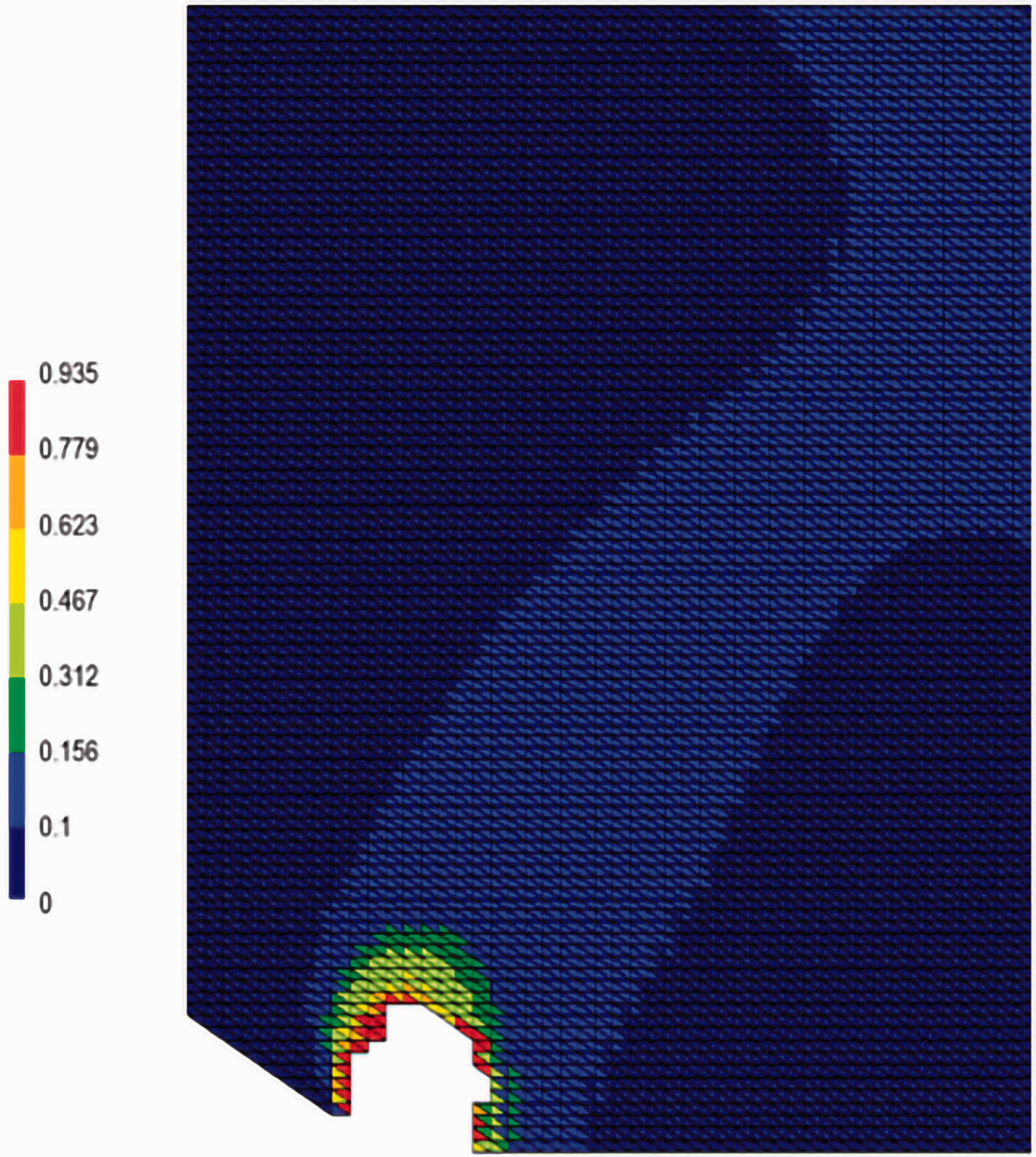
Numerical results were obtained for two FE meshes with 4276 and 9287 elements. We use uniform meshes in order to implement the possibility of satisfactory simulation of stress-strain state and damage distribution around the macrodefect stress concentrator at each stage of fracture process. This approach allows us to avoid the necessity of time-consuming process of full remeshing. The processes of damage accumulation and macrodefect development were investigated. As an examples, the shape obtained by FE model at the time moments t = 8.2 h (Figure 6), t = 10.02 h (Figure 7), t = 10.15 h (Figures 8 and 9) are presented. The distributions of damage parameter ω are given by color scale.

Figure 7.

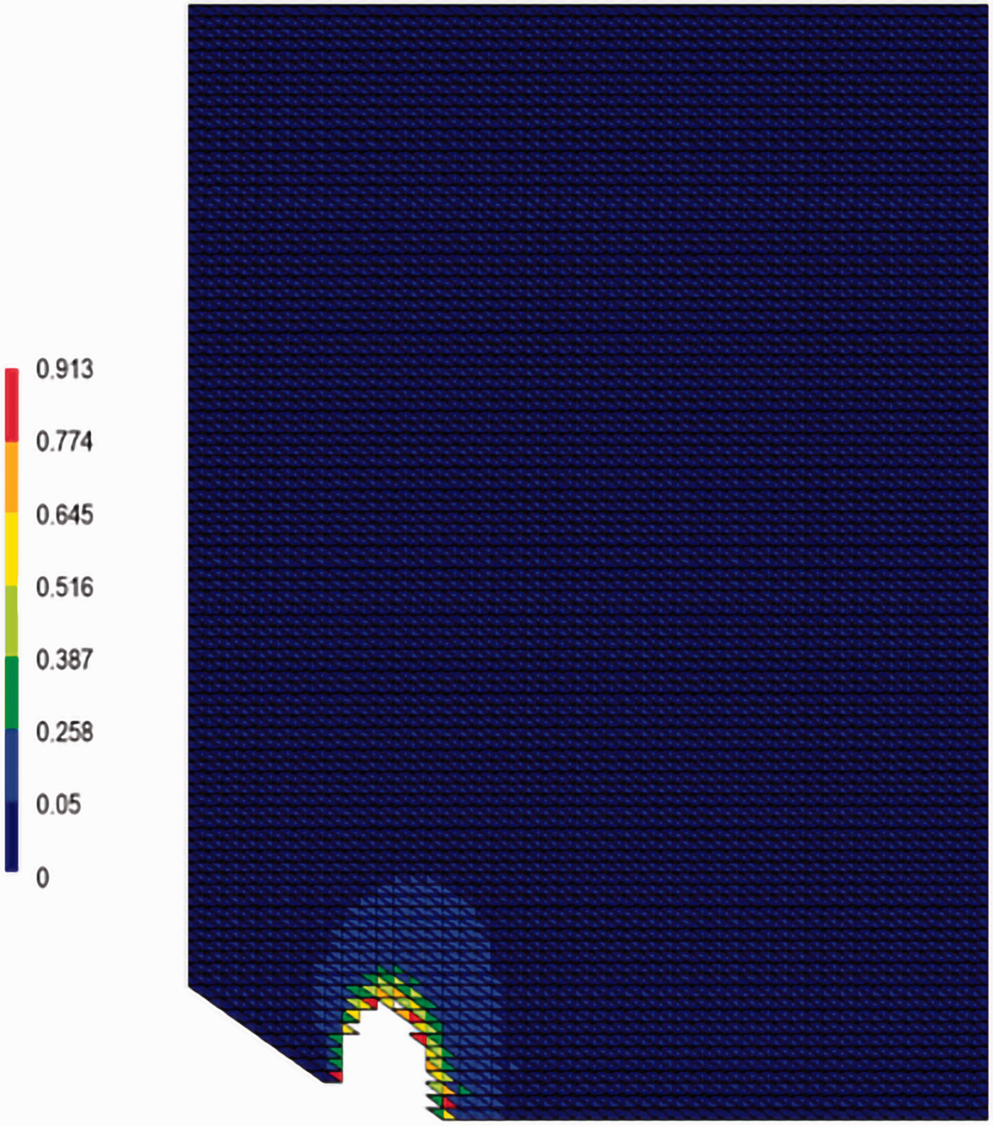
FE model of the part of the notched specimen with damage distribution during the fracture process, t = 10.02 h. Mesh with 9287 elements.

Figure 8.

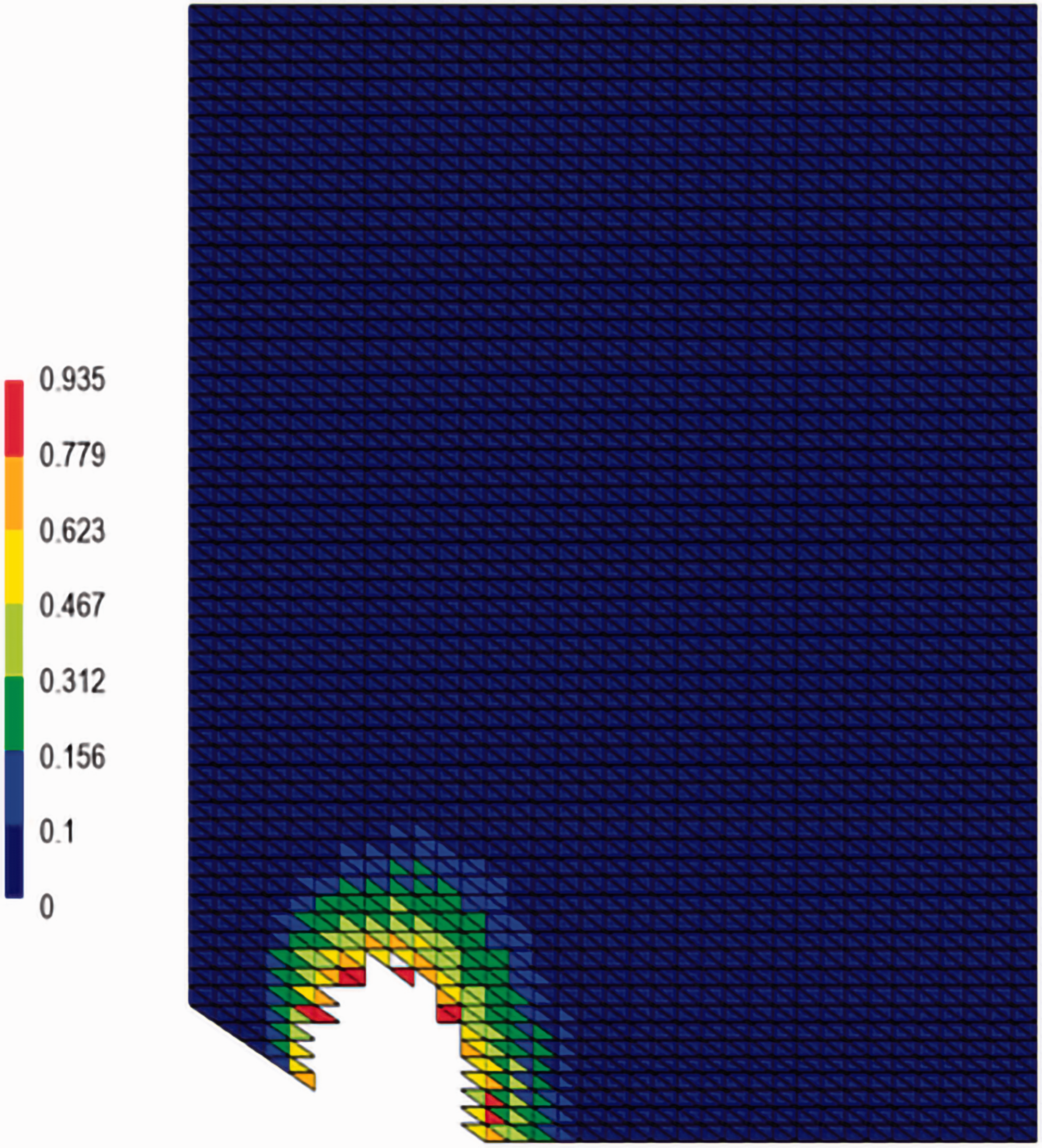
FE model of the part of the notched specimen with damage distribution during the fracture process, t = 10.15. Mesh with 4276 elements.

Figure 9.

FE model of the part of the notched specimen with damage distribution during the fracture process, t = 10.15 h. Mesh with 9287 elements.

Comparison of numerical results (see, for example Figures 8 and 9, which were obtained by use of different meshes) show, that maps of damage as well as the shape of macrodefects at the same moments of time are very close. For example, difference in their area does not exceed 15%, in values of time to fracture is 4%. As can be seen from the figures, the damage growth continues around the border of the destroyed area.

During the calculation process in some cases the meshes with finite elements going beyond the inner crack area like triangles with two free sides were obtained (Figures 8 and 10(a)). This model configuration is not physically permissible. Its use even with the remeshing will lead to the essential stress concentration. To avoid this problem the algorithm from Figure 5 (Breslavsky et al., 2018) was modernized. The idea was the smoothing the current borders of the macrodefect. The voids between edges were filled with additional elements. The fragments of the mesh around the macrodefect are presented on Figure 10 (Figure 10(a): initial configuration; Figure 10(b): improved to further calculations). Then partial remeshing algorithm was run with the procedure of node shifting in order to avoid the singularity in macrodefect contour and to reduce the stress state to the level corresponding to level of stress concentration, which would occur in the creep-damage process without fracture in a notch area. The main feature of this approach to approximate analysis of fracture is the presentation of the fracture stages as a sequence of creep-damage analysis problems for notches of different geometry (see the Method of numerical modelling section). A similar analysis of convergence for different shapes was carried out before the start of numerical investigations of fracture process. When modeling was performed by use of meshes with larger number of elements, due to a practically smooth contour of the macrodefect such algorithm was applied less often.

Figure 10.

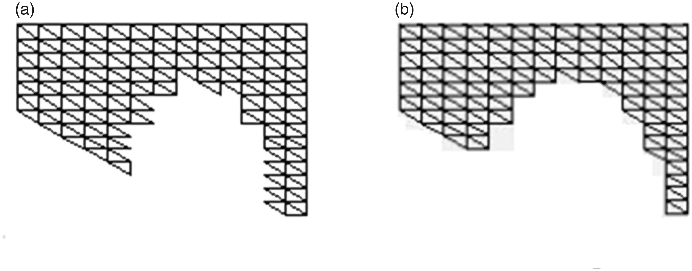
Current (a) and improved (b) parts of FE model’s fragments.

Comparison of the experimentally obtained shape of the fracture area (Figure 11(а)) with numerically obtained geometry (Figure 11(b)) allows us to conclude that they are very close. As can be seen from Figure 11(a), the crack went in diagonal direction on both sides of specimen but these directions were antisymmetric. Figure 11(b) demonstrates similar diagonal propagation of the macrodefect.

Figure 11.

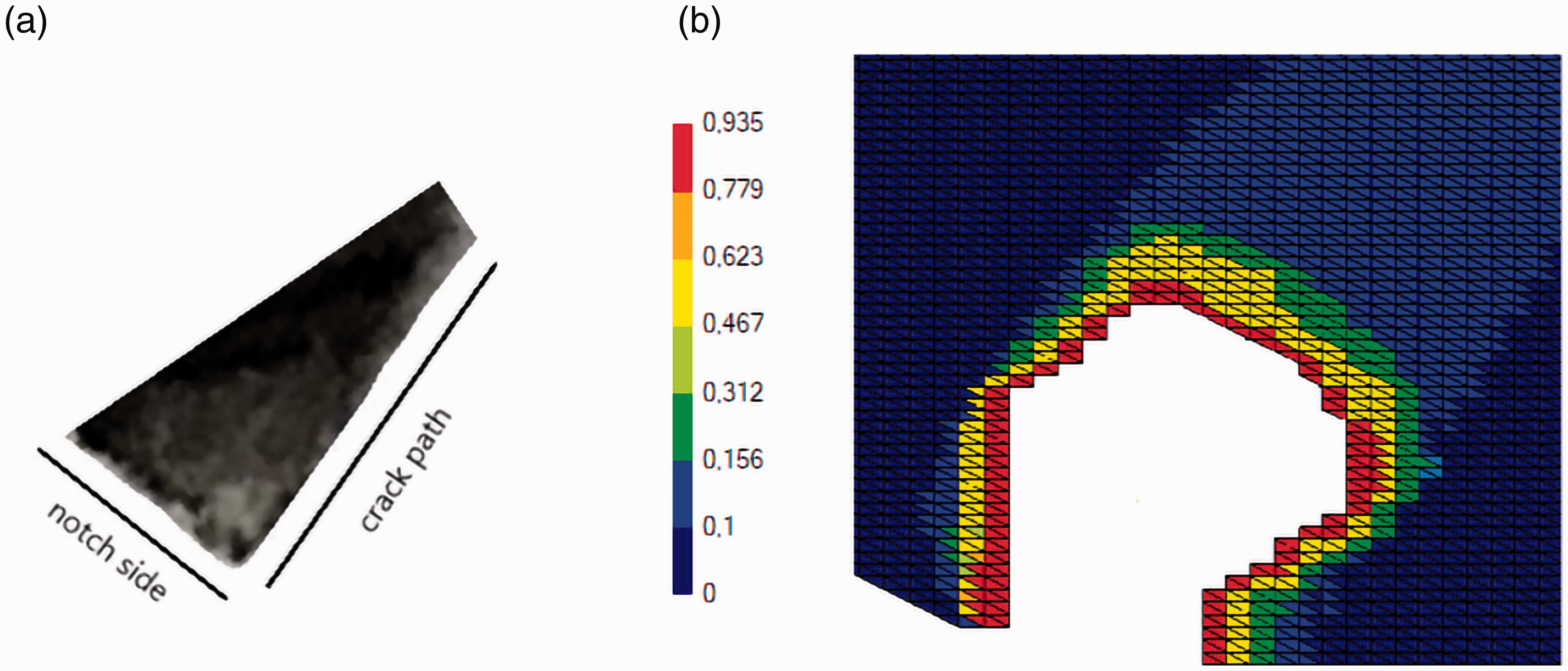
Fragments of notched specimen, character of fracture. experimental, enlarged image (a); numerical, t = 10.5 h (b).

Analysis of the damage propagation, which was performed based on the numerical results, shows that this process is characterized by growing both in axial and in normal to axial directions. Analyzing the data from Figures 6 and 7, we see that in first stages area of damage parameter’s big values are uniformly distributed around the notch tip. After that, the character of damage propagation persisted, the area of the ‘destroyed’ finite elements spread normally to the notch edge, which is in agreement with conclusion from Saanouni et al. (1986), where it was pointed out, that at first stages crack may grow at 45° angle to the specimen’s axis.

Іn this experiment due to relatively large loading, and, as a consequence, fast macrodefect development, the direction of its propagation remained diagonal. Calculations show that macrodefect propagates approximately normally to the notch border. After two hours of this propagation in experiments we have full fracture of the specimen. Results of calculations show that damage parameter reach its critical value practically in any element, situated between the macrodefect region and the edge of the specimen. That is why we can say that the first stage of development (a 45° crack orientation) due to a small period of fracture is dominant.

The obtained macrodefect is the stress concentrator, which limits the specimen’s strength. According to the numerical simulations, the further growth of the macrodefect (which already can be named crack) because of its heading to the specimen’s axial line, is not so big. The numerically obtained time (t = 10.9 h for the mesh with 4276 elements and t = 10.55 h for the mesh with 9287 elements) is the moment when the damage parameter reaches its critical value in both elements in the stripe going from current crack’s border to the axial center line of specimen. Therefore, it was determined as fracture time. The difference between experimental and numerical values of fracture times is 10–12%, which is acceptable error.

The character of fracture in these last moments of the specimen’s life is the following. After crack’s motion in the angular direction, during several seconds, all finite elements situated between fracture area and its symmetry axis obtain critical value of damage parameter.

Analyzing the data of numerical experiments, we can conclude that satisfactory results can be obtained by use of FE mesh with smaller numbers of elements but for it, it is necessary to use more frequently the procedure of mesh ‘refinement’ like demonstrated in Figure 10.

Periodic loading of the notched specimens which caused the dynamic creep process in the material led to essentially different character of fracture process. After the completion of damage growth in the notch tip (experimental value t_*=4.6 h, numerically obtained using model 1 t_*= 4.95 h, using the model 2 t_*= 4.5 h) the fast, lasting only several seconds, ‘removal’ of finite elements in notch area up to specimen’s dividing into two parts, occurred. Thus, the fracture process in the case of dynamic creep in duralumin notched specimens is characterized by the almost coincidence of the hidden damage accumulation time and the fracture time. This distinguishes the cases of static and fast periodic loading.

Generally, after the comparisons of obtained numerical and experimental data, we can conclude that the agreement between them for the case of plane stress state is good. Obtained difference in values of strains and displacements which maximum does not exceed 30% is practically usual in creep and fracture investigations. The times to fracture can be found with greater degree of accuracy, where the error is in ranges 8–12%. The last result can be regarded as significant, because the analysis of the long-term strength of structures with correspondent determination of their lifetimes is an important problem in engineering. For the moment the presented procedure has the advantage comparing with commercial software that consists in specifying the zero stiffness in ‘broken’ finite elements without their removal. Our procedure ensures the real modelling of structural element with real stiffness and boundary conditions at all stages of creep fracture process.

Conclusions

The creep-damage processes with subsequent fracture in duralumin notched specimens is studied. The cases of static and fast periodic harmonic loading which lead to static and dynamic creep correspondingly are analyzed. The initiation and growth of a macrocrack are studied using creep-damage 2 D FEA with specially developed procedure for removal of the ‘broken’ elements. The lifetime of the notched specimens is taken as a sum of two parts: the first one being the time of the hidden damage development up to the failure in a finite element. The second part is the time of the creep fracture, which is found by sequence of numerical simulations of new creep-damage boundary-initial value problems for new FE model with removed elements. The consideration of current damage redistribution in the least part of structural element is provided.

The difference in the fracture process in considered duralumin specimens for the case of static and dynamic creep is established. It was determined experimentally and numerically that in the case of pure static loading there is an essential time of the crack development (approximately 20% of total time). Instead, the oscillating load leads to the intensification of the creep-damage process. This acceleration results in the negligible duration of the second stage of fracture process. This means that for given material and conditions the dynamic creep fracture estimation can be performed only by creep-damage analysis.

The presented numerical results are examples of application of the proposed general approach and solution method of the creep-damage-fracture problems for various material properties and temperature range. The relatively short duration of experiments in 1 D and 2 D cases is determined only by the long-term strength properties in used stress range. In case of lower stress the time to fracture values will be larger but presented approach and method remain valid due to the use of common hypotheses of creep-damage theory.

The paper contains new results of the problem of fracture of solids under creep conditions and forced oscillations, which to the best of authors’ knowledge have never been obtained before. The processes of the accumulation of hidden creep damage in solids under these conditions were formerly investigated (Breslavsky et al., 2014, 2019; Lasan, 1949; Taira and Otani, 1986), but the problem of macrocrack development in the case of dynamic creep is solved for the first time. The proposed approach for solving the problem in consideration is based on the efficient technique for reducing the problem of creep under oscillating load into static one by means of asymptotic expansions and averaging over the period the problem. The innovative method for dynamic creep damage consideration in numerical simulation of oscillating structural element’s fracture is used. Both for static and dynamic creep fracture processes the developed method of changing the sequence the boundary-initial value problems with boundary conditions, which are adapted to current macrocrack region, bring good results without full remeshing of the model. This conclusion is corroborated by comparison of the experimental and numerical results.

In general, such investigations with comparison between experimental and numerical results have to be done for each type of stress concentrator (the number of them is not too large, especially for 2 D problems) for the adequate mesh to be selected. It is important for practical creep analysis due to the fact that majority of numerical results are obtained by commercial FE software where local approach is used.

The numerical and experimental results, which are presented by Breslavsky et al. (2018) allow us to recommend the developed approach and software for subsequent analysis of static and dynamic creep-damage-fracture processes in structural elements.

Footnotes

Declaration of conflicting interests

The author(s) declared no potential conflicts of interest with respect to the research, authorship, and/or publication of this article.

Funding

The author(s) received no financial support for the research, authorship, and/or publication of this article.

ORCID iD

D Breslavsky

References

Almansba

Saanouni

Hannachi

(2012) A simple damage-gradient enhanced elastoplastic formulation and its numerical implementation. Mechanics & Industry 13(2): 97–110.

Badreddine

Saanouni

Dogui

(2010) On non-associative anisotropic finite plasticity fully coupled with isotropic ductile damage for metal forming. International Journal of Plasticity 26(11): 1541–1575.

Bažant

Jirásek

(2002) Nonlocal integral formulations of plasticity and damage: Survey of progress. Journal of Engineering Mechanics 128(11): 1119–1149.

Breslavskii

Morachkovskii

(1998) Nonlinear creep and the collapse of flat bodies. International Applied Mechanics 34(3): 287–292.

Breslavsky

Chuprynin

Morachkovsky

, et al. (2019) Deformation and damage of nuclear power station fuel elements under cyclic loading. Journal of Strain Analysis for Engineering Design 54(5–6): 348–359.

Breslavsky

Kozlyuk

Tatarinova

(2018) Numerical simulation of two-dimensional problems of creep crack growth with material damage consideration. Eastern-European Journal of Enterprise Technologies 2(7): 27–33.

Breslavsky

Morachkovsky

Tatarinova

(2014) Creep and damage in shells of revolution under cyclic loading and heating. International Journal of Non-Linear Mechanics 66: 87–95.

Breslavsky

Korytko

Tatarinova

(2017) Design and Development of Finite Element Method Software. Kharkiv: Pidruchnyk NTU ‘‘KHPI” (in Ukrainian).

Brünig

Brenner

Gerke

(2015) Stress state dependence of ductile damage and fracture behavior: Experiments and numerical simulations. Engineering Fracture Mechanics 141: 152–169.

10.

Chaboche

(2002) Damage Mechanics: In Comprehensive Structural Integrity. vol. 2. Oxford: Pergamon Press, pp.213–284.

11.

Chen

Woody Ju

, et al. (2019) Influence of micro-modulus functions on peridynamics simulation of crack propagation and branching in brittle materials. Engineering Fracture Mechanics 216: 106498.

12.

Endo M and Yanase K (2018) Analysis of the Plastic Zone Size Ahead of the Crack Tip in Notched Components and Its Application to Fatigue Problems. In: Prakash R, Jayaram V and Saxena A (eds) Advances in Structural Integrity. Singapore: Springer. Available at: https://doi.org/10.1007/978-981-10-7197-3_50

13.

Erdogan

(2000) Fracture mechanics. International Journal of Solids and Structures 37(1–2): 171–183.

14.

Hallquist

(2005) LS DYNA Theoretical Manual. Livermore: Livermore Software Technology USA Corporation.

15.

Hayhurst

Brown

Morrison

(1984) The role of continuum damage in creep crack growth. Philosophical Transactions of the Royal Society of London. Series A Mathematical and Physical Sciences 311(1516): 131–158.

16.

Hayhurst DR, Horrison CJ and Brown PR (1981) Creep crack growth. In: 3rd symposium Creep in structures (eds ARS Ponter and DR Hayhurst) Leicester, UK, 8-12 September 1980, pp. 564-575. NY: Springer.

17.

Jing

, et al. (2017) Finite element simulation of creep fatigue crack growth behavior for P91 steel at 625°C considering creep-fatigue interaction. International Journal of Fatigue 98: 41–52.

18.

Kim

Lee

(2001) Behavior of plasticity-induced crack closure and roughness-induced crack closure in aluminum alloy. International Journal of Fatigue 23: 247–251.

19.

Konkin

Morachkovskii

(1987) Creep and long-term strength of light alloys with anisotropic properties. Strength of Materials 19(5): 626–631.

20.

Lasan

(1949) Dynamic creep and rupture properties of temperature-resistant materials under tensile fatigue stress. In: Proceedings of the ASTM, vol. 49, pp.757–787.

21.

Lemaitre

Chaboche

(1994) Mechanics of Solid Materials. Cambridge: Cambridge University Press.

22.

Gao

Liu

(2019) A mesh objective continuum damage model for quasi-brittle crack modelling and finite element implementation. International Journal of Damage Mechanics 28(9): 1299–1322.

23.

Liu W, Saanouni K, Laberg_ere C, et al. (2016) Nonlocal constitutive equations of elasto-visco-plasticity coupled with damage and temperature. In: 12th international conference on numerical methods in industrial forming processes, MATEC web of conferences, vol. 80. Available at: https://www.matec-conferences.org/articles/matecconf/abs/2016/43/matecconf_numi2016_01002/matecconf_numi2016_01002.html

24.

Lokoshchenko

Shesterikov

(1980) Method for description of creep and long-term strength with pure elongation. Journal of Applied Mechanics and Technical Physics 21(3): 414–417.

25.

Mengjia

Junmei

Hao

, et al. (2016) Effects of residual stress and grain boundary character on creep cracking in 2.25Cr-1.6W steel. Materials Science & Engineering, A 659: 188–197.

26.

Ohtani R (1981) Finite Element Analysis and Experimental Investigation on Creep Crack Propagation. In: Ponter ARS and Hayhurst DR (eds) Creep in Structures. International Union of Theoretical and Applied Mechanics. Berlin, Heidelberg: Springer. Available at: https://doi.org/10.1007/978-3-642-81598-0_36

27.

Pandey

Singh

Mishra

, et al. (2019) Creep crack simulations using continuum damage mechanics and extended finite element method. International Journal of Damage Mechanics 28(1): 3–34.

28.

Paris

Saanouni

(2011) Damaged behavior under plane stress, numerical integration of elasto-viscoplastic-damage constitutive equations under plane stress condition. European Journal of Computational Mechanics 20(5–6): 341–368.

29.

Penny

Marriott

(1995) Design for Creep. London: Chapman & Hall.

30.

Perrin

Hayhurst

(1999) Continuum damage mechanics analyses of type IV creep failure in ferritic steel crossweld specimens. International Journal of Pressure Vessels and Piping 76(9): 599–617.

31.

Riedel H (1989) Creep Crack Growth. In: Wei R and Gangloff R (eds) Fracture Mechanics: Perspectives and Directions (Twentieth Symposium). West Conshohocken, PA: ASTM International, 101–126. Available at: https://doi.org/10.1520/STP18822S

32.

Saanouni

Chaboche

Bathias

(1986) On the creep crack growth prediction by a local approach. Engineering Fracture Mechanics 25(5–6): 677–691.

33.

Scheider

Schödel

Brocks

, et al. (2006) Crack propagation analyses with CTOA and cohesive model: Comparison and experimental validation. Engineering Fracture Mechanics 73(2): 252–263.

34.

Taira

Otani

(1986) Theory of High-Temperature Strength of Materials. Moscow: Metallurgiya (in Russian).

35.

Traidia

Alfano

Lubineau

, et al. (2012) An effective finite element model for the prediction of hydrogen induced cracking in steel pipelines. International Journal of Hydrogen Energy 37(21): 16214–16230.

36.

Voyiadjis

Oucif

Kattan

, et al. (2020) Damage and healing mechanics in plane stress, plane strain, and isotropic elasticity. International Journal of Damage Mechanics 29(8): 1246–1270.

37.

Walczak

Sieniawski

Bathe

K-J

(1983) On the analysis of creep stability and rupture. Computers & Structures 17(5–6): 783–792.

38.

Wyart

Coulon

Duflot

, et al. (2007) A substructured FE shell/XFE3D method for crack analysis in thin-walled structures. International Journal for Numerical Methods in Engineering 72(7): 757–779.

39.

Yatomi

Davies

Nikbin

(2008) Creep crack growth simulations in 316H stainless steel. Engineering Fracture Mechanics 75(18): 5140–5150.

40.

Yatomi

Nikbin

O’Dowd

(2003) Creep crack growth prediction using a damage based approach. International Journal of Pressure Vessels and Piping 80(7–8): 573–583.

41.

Zhao

Nikbin

(2017) Predicting failure modes in creep and creep-fatigue crack growth using a random grain/grain boundary idealised microstructure meshing system. Materials Science and Engineering: A 704: 274–286.