A simple implementation of localizing gradient damage model in Abaqus

Abstract

With the localizing gradient enhancement, a damage model for quasi-brittle materials is able to achieve regularized softening responses, with localized damage profiles corresponding to the development of macroscopic cracks, to resolve the numerical spurious effects induced by the conventional gradient enhancement. The typical implementation strategy for a gradient enhanced model is to solve the system of governing equations simultaneously. Focusing on the finite element (FE) package Abaqus, a user element subroutine is required to define the finite elements with additional degrees of freedom for the nonlocal field. Moreover, with user elements, additional effort is required to visualize the numerical results. To an inexperienced engineer/researcher, these requirements can be challenging. In this paper, a simple implementation of the localizing gradient damage model is elaborated. By utilizing the in-built coupled thermo-mechanical elements in Abaqus, the user only needs to define the material constitutive laws, as well as the sensitivity terms with respect to the field variables. Post-processing of results can be done directly in Abaqus. The applicability and ease of implementation are demonstrated via several examples, including those that utilize the Abaqus features of element deletion, contact between surfaces, as well as the incorporation of cohesive elements. Sample files can be downloaded from https://github.com/leonghien/Localizing-Gradient-Damage-with-UMAT-UMATHT

Keywords

Localizing gradient damage coupled thermo-mechanical analysis quasi-brittle fracture Abaqus

Introduction

The nonlocal gradient enhancement is widely used to regularize the strain softening behavior of continuum damage models. Typically, a higher order balance equation is incorporated in the formulation to capture the interactions between micro-cracks, with a length scale parameter characterizing the size of fracture process zone. The conventional gradient enhancement, however, suffers from a spurious damage growth phenomenon. This has led to the development of a so-called localizing gradient enhancement, to give sharp damage profiles corresponding to the development of macroscopic cracks. Numerically, the system of governing equations defining equilibrium and higher order balance in a gradient enhancement is commonly solved simultaneously, using finite elements (FE) with additional degrees of freedom (dof). The need for additional dofs complicates its implementation into the standard FE framework of commercial FE software. In this paper, we present a simple implementation of the localizing gradient enhancement in the commercial FE software Abaqus, by utilizing its in-built elements for coupled thermo-mechanical analyses.

The conventional nonlocal enhancement was first proposed as an integral-type formulation (Pijaudier-Cabot and Bažant, 1987), where the influence of underlying micro-processes is captured via the spatial averaging of the driving field within the damage process zone. While the nonlocal integral approach has been adopted successfully for many problems (Havlásek et al., 2016; Jirásek and Desmorat, 2019; Pereira et al., 2017), its numerical implementation in a standard FE framework can be difficult. The gradient approach forms another big class of nonlocal enhancement, which can be understood as a reformulation of the integral enhancement (Peerlings et al., 1996, 1998, 2001). Here, a higher order balance equation governs the evolution of the nonlocal field, to drive the damage process. This additional differential equation can be assimilated into a standard FE framework more easily than the integral approach, and is thus widely adopted to regularize the softening response (Ahmed et al., 2021a, 2021b; Mobasher et al., 2017; Schreter et al., 2018; Zreid and Kaliske, 2018). While the conventional nonlocal enhancement is able to regularize the structural response well, both the integral and gradient approaches induce numerical artefacts such as a wrong damage initiation and propagation behavior (Geers et al., 1998; Giry et al., 2011; Nguyen, 2011; Simone et al., 2004), or a spurious boundary effect resulting in an inability to reproduce the size effect phenomenon of quasi-brittle fracture (Grégoire et al., 2013; Havlásek et al., 2016; Marzec and Bobiński, 2019; Wosatko et al., 2018). This has motivated the development of localizing gradient enhancement, where the energetic contribution from active micro-process zone decreases with damage evolution, to result in a slightly modified higher order balance equation compared to the conventional expression (Poh and Sun, 2017). The localizing gradient enhancement was shown to work well for different problems, e.g. quasi-static fracture of quasi-brittle materials (Castillo et al., 2021; Sarkar et al., 2019; Shedbale et al., 2021; Tong et al., 2021b), size effects in quasi-brittle fracture (Negi et al., 2021; Zhang et al., 2021), thermo-mechanical fracture (Sarkar et al., 2020), continuous-discontinuous modelling (Sarkar et al., 2021), dynamic fracture (Wang et al., 2019) and ductile fracture (Xu et al., 2020; Xu and Poh, 2019).

The gradient enhancement is typically solved as a system of equations in the weak form. While the numerical framework can be derived easily with only C⁰ continuity requirement, its implementation in a commercial FE software can be complicated, especially to an inexperienced researcher/engineer. Focusing specifically on the FE software Abaqus, the common strategy is to write a user element (UEL) subroutine to define additional dofs, as well as to determine the elemental contribution to the overall tangent stiffness matrix and residual force vector. The writing of UEL can be cumbersome for practical applications, especially when a new subroutine has to be written whenever there is a change in shape function and/or element type. Moreover, the visualization of UEL analyses in Abaqus has to be done indirectly, e.g. with an overlaying mesh of standard elements generated during the pre-processing stage (Sarkar et al., 2019; Tong et al., 2021a, 2021b), or having a script to extract the relevant result data and updating an odb file generated from dummy Abaqus in-built elements (Roth et al., 2012).

In the literature, there are attempts to simplify the implementation of the conventional gradient enhancement in Abaqus. The general approach is to utilize the in-built coupled temperature-displacement elements in Abaqus. Since the higher-order term in the balance equation of conventional gradient enhancement involves only a Laplacian term, it is analogous to the heat equation assuming Fourier’s law, where the heat flux is linearly dependent on the temperature gradient. In Abaqus, such thermo-mechanical analyses can be implemented conveniently using the UMAT and HETVAL subroutines to define the mechanical constitutive laws and heat flux relation respectively. A proper definition of parameters in HETVAL subroutine will recover the balance equation in conventional gradient enhancement, with the temperature field corresponding to the nonlocal variable. This strategy has been utilized successfully for damage modelling (Azinpour et al., 2018), and plasticity-driven ductile fracture (Papadioti et al., 2019; Seupel et al., 2018). Although not necessary, the more general UMATHT subroutine was utilized by Ostwald et al. (2019) to define the linear (thermal) flux relation, in their implementation of the conventional gradient enhancement for a large deformation isotropic hyperelastic damage model. It is also worth mentioning that the same strategy has been adopted by researchers to implement the phase field fracture models, another large class of regularization method. Since the higher order term in the phase field model also involves only a Laplacian term, the parameters in HETVAL subroutine can similarly be redefined to recover the phase field balance equation (e.g. Azinpour et al., 2018; Navidtehrani et al., 2021; Wu and Huang, 2020).

The simplified Abaqus implementation of conventional gradient enhancement/phase field damage models has motivated us to consider a similar strategy for the localizing gradient enhancement. Since the higher order term in the localizing gradient enhancement involves the divergence of a nonlinear flux relation, the HETVAL subroutine that is applicable for (linear) Fourier’s law cannot be utilized here. Departing from the common strategy by other researchers, the more general UMATHT subroutine is adopted in this paper for defining the nonlinear flux relation, to recover the localizing gradient enhancement balance equation. The paper is structured as follows. A summary of the localizing gradient damage model is provided in the next section. In Section ‘Implementation using UMAT-UMATHT subroutines’, the analogy between a coupled thermo-mechanical analysis and the localizing gradient enhancement is elaborated, and implementation details via the UMAT-UMATHT subroutines provided. In Section ‘Validation and discussions with compact tension specimen’, a validation of the proposed simplified implementation approach is demonstrated, and the ease of analysis in conjunction with other Abaqus in-built features illustrated in Section ‘Numerical examples considering other Abaqus in-built features’. Finally, the model extension to 3D is provided by taking advantage of the simplified implementation approach, and its good performance in capturing non-planar mixed mode fracture behavior demonstrated in Section ‘3D modelling of prismatic skew edge notched beam in torsion’.

Summary of the localizing gradient damage enhancement

In this section, a brief summary of the localizing gradient damage model is provided. Detailed discussions can be found in Poh and Sun (2017).

Governing equations and constitutive relations

For a given strain rate $\dot{ε}$ , the internal power statement is postulated as

P_{int} = \int_{R} (σ : \dot{ε} + \tilde{σ} \dot{\tilde{e}} + \tilde{ξ} \cdot \nabla \dot{\tilde{e}}) dV

(1)

where

σ

denotes the standard Cauchy stress. Additional contributions are associated with a micromorphic strain

\dot{\tilde{e}}

and its gradient characterizing the deformation in the (micro) damage process zone, together with the respective conjugate stresses

\tilde{σ}

and

\tilde{ξ}

The external power is given by

P_{ext} = \int_{\partial R} (t \cdot \dot{u} + ζ \dot{\tilde{e}}) dA

(2)

where t and ζ are respectively the traction and higher-order traction acting at the boundary.

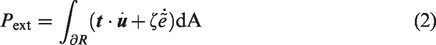
Equating $P_{int} = P_{ext}$ and applying the divergence theorem, we obtain a system of governing equations given by the standard equilibrium condition, as well as a higher order balance equation

\nabla \cdot σ = 0, \tilde{σ} = \nabla \cdot \tilde{ξ}

(3)

The tractions at the external boundary with outward normal n are also determined as $t = σ \cdot n$ and $ζ = \tilde{ξ} \cdot n$ .

The free energy density comprises the elastic strain energy of the undamaged material, augmented by a coupling contribution between macro and micro deformations, which are respectively characterized by an equivalent macro strain measure e and a scalar micro strain $\tilde{e}$ . Moreover, an additional contribution arises from the interactions between active micro processes characterized via $\nabla \tilde{e}$ , to give

ψ = \frac{1}{2} (1 - ω) ε : C : ε + \frac{1}{2} \tilde{h} {(e - \tilde{e})}^{2} + \frac{1}{2} g \tilde{h} l^{2} \nabla \tilde{e} · \nabla \tilde{e}

(4)

where

C

is the forth-order elastic stiffness tensor,

0 \leq ω \leq 1

an isotropic damage variable capturing the extent of material degradation,

\tilde{h}

a coupling modulus accounting for the micro-macro interactions, and l a length scale parameter characterizing the initial size of damage process zone.

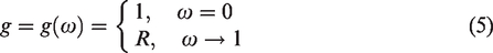
Note that an interaction function g is appended to the energetic contribution from the interactions between active micro cracks. Since the failure process typically involves an initially diffused region of micro cracks before transiting into localized macro cracks, the interaction function has the following characteristics

g = g (ω) = {\begin{array}{l} 1, ω = 0 \\ R, ω \to 1 \end{array}

(5)

where

R \approx 0

describes a residual interaction between micro-processes. In this paper, the interaction function proposed in Poh and Sun (2017) is adopted

g = \frac{(1 - R) \exp (- η ω) + R - \exp (- η)}{1 - \exp (- η)}

(6)

where η is a material parameter describing the rate which the interaction domain decreases with damage. Discussions on the influence of R and η can be found in Sarkar et al. (2019). In the following,

R = 0.005

and η = 5 are utilized for all examples.

From the Coleman-Noll procedure, the constitutive relations are determined as

σ = \frac{\partial ψ}{\partial ε} = (1 - ω) C : ε + \tilde{h} (e - \tilde{e}) \frac{\partial e}{\partial ε}

(7a)

\tilde{σ} = \frac{\partial ψ}{\partial \tilde{e}} = \tilde{h} (\tilde{e} - e)

(7b)

\tilde{ξ} = \frac{\partial ψ}{\partial \nabla \tilde{e}} = g \tilde{h} l^{2} \nabla \tilde{e}

(7c)

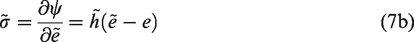
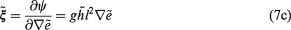
Following Sarkar et al. (2019), the coupling modulus $\tilde{h}$ is assumed to be much smaller than the Young’s modulus, such that the standard constitutive relation for a strain driven damage model is recovered, i.e.

σ = (1 - ω) C : ε

(8)

The microforce balance governing the micro-macro interactions is also obtained by substituting equations (7b) and (7c) into equation (3b), to give

\tilde{e} - e = \nabla \cdot (g l^{2} \nabla \tilde{e})

(9)

This balance equation defines the localizing gradient enhancement. Note that the conventional gradient enhancement is recovered for the special case of a constant interaction size, i.e. g = 1.

Equivalent strain measure and damage evolution

To complete the model definition, an equivalent strain measure (e) that can adequately characterize the underlying deformation state is required, together with a suitable damage evolution law. A detailed discussion on some common equivalent strain measures for the mixed mode fracture of quasi-brittle materials can be found in Shedbale et al. (2021).

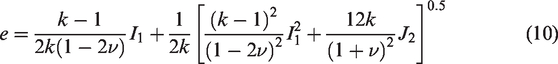
In this paper, the modified von Mises equivalent strain measure (de Vree et al., 1995) is adopted, defined as

e = \frac{k - 1}{2 k (1 - 2 ν)} I_{1} + \frac{1}{2 k} {[\frac{{(k - 1)}^{2}}{{(1 - 2 ν)}^{2}} I_{1}^{2} + \frac{12 k}{{(1 + ν)}^{2}} J_{2}]}^{0.5}

(10)

where ν is Poisson’s ratio, and k is a material parameter characterizing the ratio between compressive and tensile strengths. The first and second strain invariants are respectively given as

I_{1} = tr (ε), J_{2} = \frac{1}{2} ε^{dev} : ε^{dev}

(11)

In addition, we adopt a commonly utilized exponential damage evolution law, given by

ω = ω (κ) = {\begin{array}{l} 0 & if κ < κ_{0} \\ 1 - \frac{κ_{0}}{κ} {1 - α + α \exp [- β (κ - κ_{0})]} & if κ \geq κ_{0} \end{array}

(12)

where α and β are material parameters controlling the residual stress and the rate of softening respectively, κ₀ is a damage initiation threshold, and κ is a history variable following the Kuhn-Tucker relations

\dot{κ} \geq 0, \tilde{e} - κ \leq 0, \dot{κ} (\tilde{e} - κ) = 0

(13)

In this paper, we adopt α = 1 for all examples shown.

The numerical implementation details of this model in Abaqus using UEL subroutines, as well as the subsequent visualization method, can be found in Sarkar et al. (2019). Below, a simpler approach is demonstrated.

Implementation using UMAT-UMATHT subroutines

The localizing gradient enhancement can be implemented easily in Abaqus, by taking advantage of its capability to solve thermo-mechanical problems with user defined relations, via the UMAT and UMATHT subroutines. This is elaborated below.

Heat equation

The general heat equation is given by

ρ c \dot{θ} = - \nabla \cdot f + r

(14)

where ρ is the material density, c is the specific heat capacity, θ is the temperature field, f is a heat flux vector, and r is the spatial heat source.

If the Fourier’s law is assumed, the heat flux vector will be linearly dependent on the temperature gradient, i.e.

f = - k \nabla θ

(15)

where k is a thermal conductivity constant. Substituting this into equation (14) will result in a Laplacian term in the heat equation, which bears similarity to the conventional gradient enhancement (where g = 1 in equation (9)), as well as the balance equation in phase field damage models. This resemblance was exploited in Azinpour et al. (2018); Navidtehrani et al. (2021); Wu and Huang (2020); Seupel et al. (2018) in their implementations of the conventional gradient enhancement/phase field damage models, using the HETVAL subroutine.

A more general heat flux constitutive relation can be considered in equation (15) by defining the thermal conductivity as a function of temperature, i.e. $k = k (θ)$ . Substituting this into equation (14) results in the following balance equation

ρ c \dot{θ} = \nabla \cdot (k (θ) \nabla θ) + r

(16)

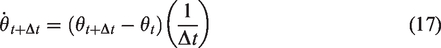
Since a nonlinear constitutive relation for heat flux is involved, the HETVAL subroutine cannot be utilized for the analysis. Instead, the more general UMATHT subroutine has to be adopted, which is the approach in this paper. In Abaqus, the time integration is done using a backward-difference scheme, i.e.

{\dot{θ}}_{t + Δ t} = (θ_{t + Δ t} - θ_{t}) (\frac{1}{Δ t})

(17)

The general strategy is to redefine the terms in the heat equation to (almost) recover the gradient enhancement balance equation, such that the temperature field $(θ)$ can be interpreted as the non-local field $\tilde{e}$ . First, the spatial heat supply term (r) in UMATHT is defined via the RPL¹ variable in UMAT as

r_{pl} = e - θ

(18)

Next, the thermal conductivity parameter is made dependent on the temperature field, defined as

k (θ) = g (θ) l^{2}

(19)

where

g = g (θ)

is the interaction function in equation (6), and l the length scale parameter in equation (9).

Substituting equations (18) and (19) into equation (16), the modified heat equation is obtained as

ρ c \dot{θ} = \nabla \cdot (g l^{2} \nabla θ) + e - θ

(20)

Comparing between equations (9) and (20), it is easily observed that the steady state heat equation recovers the localizing gradient balance equation, with θ as an analogous field to $\tilde{e}$ . For the transient analysis, a steady state approximation can be achieved numerically by setting the term ‘ρc’ to a small value. In the original heat diffusion problem, parameter c denotes the specific heat capacity with units of J/kg/K. In the modified diffusion equation resembling the localizing gradient governing equation, the combined term ρc has unit of s, which represent a characteristic time. For all problems, the default loading time for quasi-static analysis (T = 1) is utilized. Discussions of the loading rate effect on the numerical solution are provided in Appendix 1. To avoid confusion, we shall assume ρ = 1 and simply state the small value of c in the following. The influence of parameter c is discussed later in Section ‘Validation and discussions with compact tension specimen’.

Numerical implementation in Abaqus

The localizing gradient enhanced damage model can now be implemented easily in Abaqus, using the UMAT and UMATHT subroutines to respectively specify the mechanical and thermal constitutive relations, as well as the tangent contributions, for a Gauss point underlying an element. The assembly of contributions from each Gauss point at the element level, which is then used to build the global system of equations, is done internally by Abaqus. Compared to the typical implementation of gradient enhanced models using the user element subroutine UEL, the adoption of UMAT-UMATHT subroutines greatly simplifies the implementation requirements. For ease of reference to the localizing gradient damage model summarized in Section ‘Summary of the localizing gradient damage enhancement’, the temperature field θ in the thermo-mechanical element will be written as its analogous field $\tilde{e}$ , in the elaborations below.

A flowchart of the UMAT-UMATHT implementation is depicted in Figure 1. Focusing first on UMAT, the stress constitutive relation has to be specified, which referring to equation (8) gives

STRESS \overset{def}{=} σ = (1 - ω) C : ε

(21)

Figure 1.

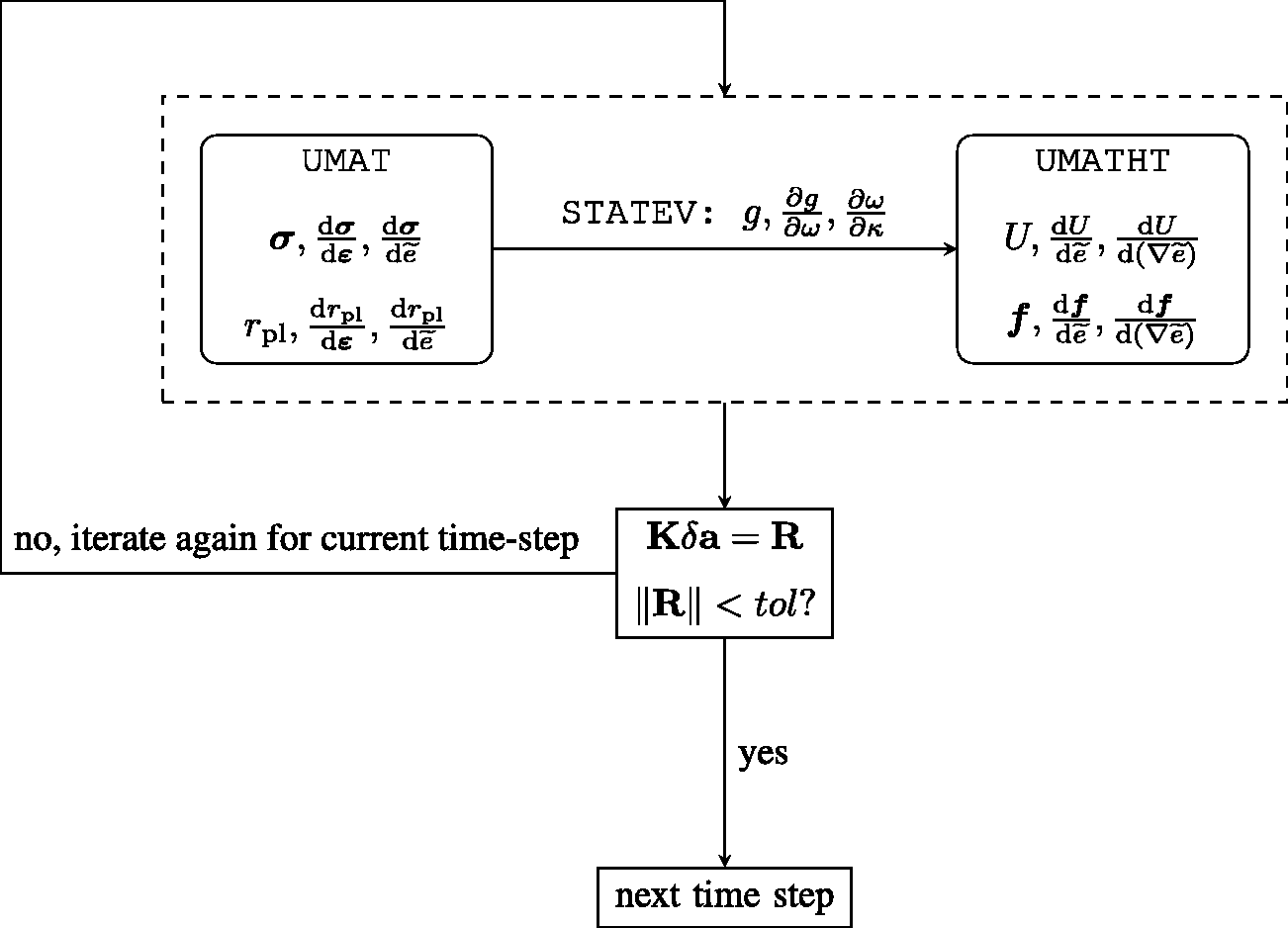
Flowchart of the UMAT-UMATHT implementation, where K is the tangent stiffness matrix, $δ a$ is the vector of incremental nodal degrees of freedom, and R is the residual force vector. Variables to be computed in UMAT are defined in equations (21) to (24). Solution dependent variables to be computed in UMAT and stored in the STATEV array, as per equations (6), (25), are passed into UMATHT. Finally, the variables to be defined in UMATHT are provided in equations (26) to (29).

The corresponding tangent contributions with respective to the field variables are obtained as

DDSDDE \overset{def}{=} \frac{d σ}{d ε} = (1 - ω) C

(22a)

DDSDDT \overset{def}{=} \frac{d σ}{d \tilde{e}} = - \frac{\partial ω}{\partial κ} C : ε

(22b)

Additionally, Abaqus expects information on the mechanical heat generation and the associated sensitivity terms to be provided in UMAT. The mechanical heat source is represented by the variable RPL, defined as

RPL \overset{def}{=} r_{pl} = e - \tilde{e}

(23)

The sensitivity of $r_{pl}$ with respect to the field variables are correspondingly

DRPLDE \overset{def}{=} \frac{d r_{pl}}{d ε} = \frac{\partial e}{\partial ε}

(24a)

DRPLDT \overset{def}{=} \frac{d r_{pl}}{d \tilde{e}} = - 1

(24b)

Finally, the sensitivity of f with respect to the field variables, to be defined later in UMATHT in equation (29), will involve some terms to be passed from UMAT. At each iterative step, the interaction function g defined in equation (6) and the following variables are computed in UMAT

\frac{\partial g}{\partial ω} = \frac{η (R - 1)}{1 - \exp (- η)} \exp (- η ω)

(25a)

\frac{\partial ω}{\partial κ} = α β \frac{κ_{0}}{κ} \exp [- β (κ - κ_{0})] + \frac{κ_{0}}{κ^{2}} {1 - α + α \exp [- β (κ - κ_{0})]}

(25b)

These solution dependent variables are stored in the array STATEV of UMAT, which will be passed to UMATHT. The variables to be specified and computed in UMAT are thus completed at this juncture.

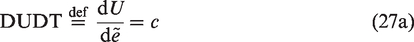
Referring to the flowchart in Figure 1, we now focus on the definitions required in UMATHT based on the transient heat equation in (20). Within this subroutine, the internal energy per unit mass U and the heat flux vector f have to be specified, as well as their sensitivities with respect to the field variables.

The internal energy is defined as a linear function of $\tilde{e}$ with a constant specific heat capacity c

U \overset{def}{=} U = c \tilde{e}

(26)

The corresponding sensitivities with respect to the field variables are thus

DUDT \overset{def}{=} \frac{d U}{d \tilde{e}} = c

(27a)

DUDG \overset{def}{=} \frac{d U}{d (\nabla \tilde{e})} = 0

(27b)

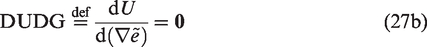
The heat flux vector is defined as

FLUX \overset{def}{=} f = - g l^{2} \nabla \tilde{e}

(28)

with the corresponding sensitivities as

DFDT \overset{def}{=} \frac{d f}{d \tilde{e}} = - l^{2} \frac{\partial g}{\partial ω} \frac{\partial ω}{\partial κ} \nabla \tilde{e}

(29a)

DFDG \overset{def}{=} \frac{d f}{d (\nabla \tilde{e})} = - g l^{2} I

(29b)

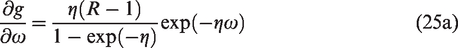
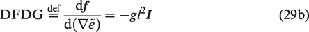
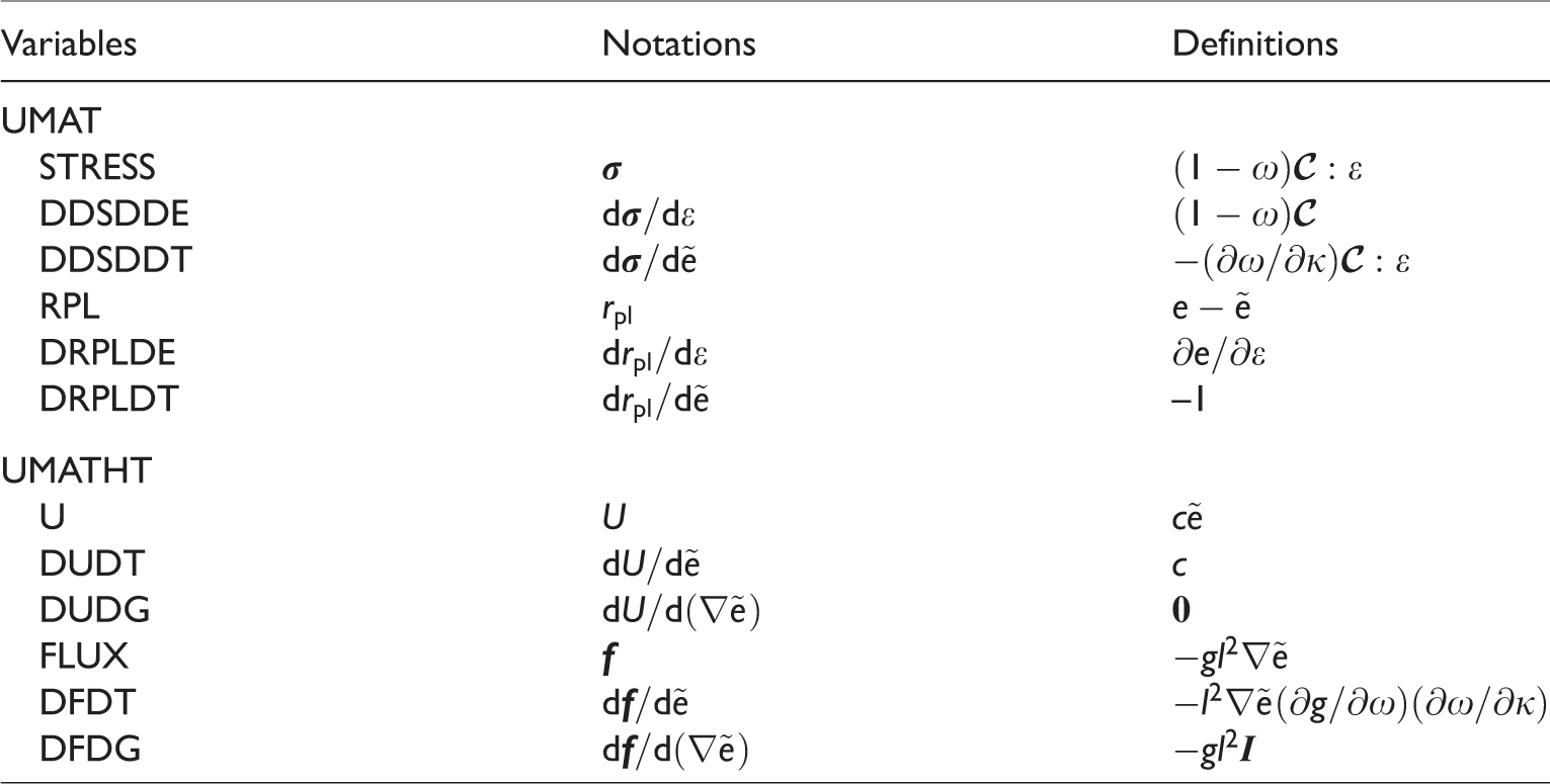
Recall that the solution dependent variables g, $\frac{\partial g}{\partial ω}$ and $\frac{\partial ω}{\partial κ}$ are obtained from UMAT in equations (6) and (25), and I is the identity matrix.

A summary of the variables to be returned in the UMAT and UMATHT subroutines is listed in Table 1.

Table 1.

Summary of the variables to be defined in UMAT-UMATHT subroutines.

Variables	Notations	Definitions
UMAT
STRESS	$σ$	$(1 - ω) C : ε$
DDSDDE	$d σ / d ε$	$(1 - ω) C$
DDSDDT	$d σ / d \tilde{e}$	$- (\partial ω / \partial κ) C : ε$
RPL	$r_{pl}$	$e - \tilde{e}$
DRPLDE	$d r_{pl} / d ε$	$\partial e / \partial ε$
DRPLDT	$d r_{pl} / d \tilde{e}$	–1
UMATHT
U	U	$c \tilde{e}$
DUDT	$d U / d \tilde{e}$	c
DUDG	$d U / d (\nabla \tilde{e})$	$0$
FLUX	f	$- g l^{2} \nabla \tilde{e}$
DFDT	d f $/ d \tilde{e}$	$- l^{2} \nabla \tilde{e} (\partial g / \partial ω) (\partial ω / \partial κ)$
DFDG	d f $/ d (\nabla \tilde{e})$	$- g l^{2} I$

Validation and discussions with compact tension specimen

In this section, we consider the mode I fracture of a compact tension specimen (CTS) with a pre-existing sharp crack, and benchmark the results from the UMAT-UMATHT implementation against those reported in Poh and Sun (2017) using UEL.

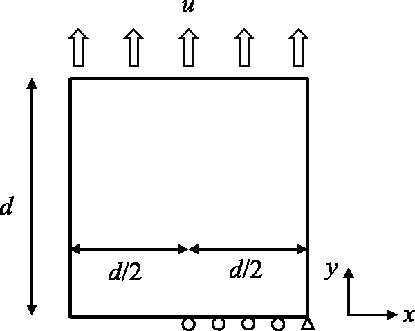
The CTS of dimension d × d is depicted in Figure 2. Here, we adopt the same material parameters as Poh and Sun (2017), where E = 1 GPa, $ν = 0.2$ , k = 10, $κ_{0} = 0.002$ , β = 9 and $l = 0.2 d$ . Plane strain condition is assumed.

Figure 2.

Geometry and boundary conditions of the CTS. Only half of the specimen geometry is considered due to symmetry about y = 0.

Plane strain analysis

We first consider the CPE8T plane strain element (8-node element with biquadratic displacement and bilinear $\tilde{e}$ ). As highlighted in equation (20), the transient term has to be made negligible (achieved by having a small value for parameter c) in order to recover the localizing gradient enhancement balance equation.

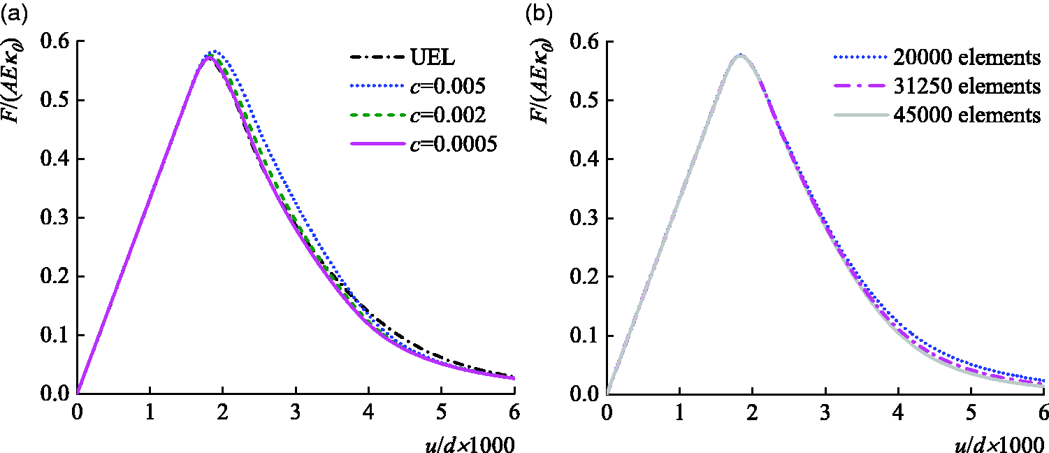
The structural responses with different specific heat capacity values of c = 0.005, 0.002 and 0.0005 are depicted in Figure 3(a). It is easily observed that a better match with the reference UEL solution is achieved, when the value for c decreases. The damage profiles at the final loading stage ( $u = 0.006 d$ ) are also provided in Figure 4(a). Again, the damage profiles compare well with the reference UEL solution, to give a localized damage band ahead of the pre-existing crack tip. As expected, the smallest value for c produces a damage profile that is almost identical to that of UEL model. In general, as long as parameter c is small, the results will not be significantly affected by the loading rate. It is shown in Figure 3(a) and Figure 4(a) that c = 0.005 is already a small enough value, to induce a marginal rate effect. The rate effect becomes negligible for c < 0.002. For generic problems, without performing preliminary sensitivity studies of parameter c, we recommend adopting c < 0.002.

Figure 3.

Structural responses using (a) CPE8T elements with different c values and (b) mesh convergence analysis using CPE3T elements with c = 0.002. The UEL reference solution is obtained from Poh and Sun (2017).

Figure 4.

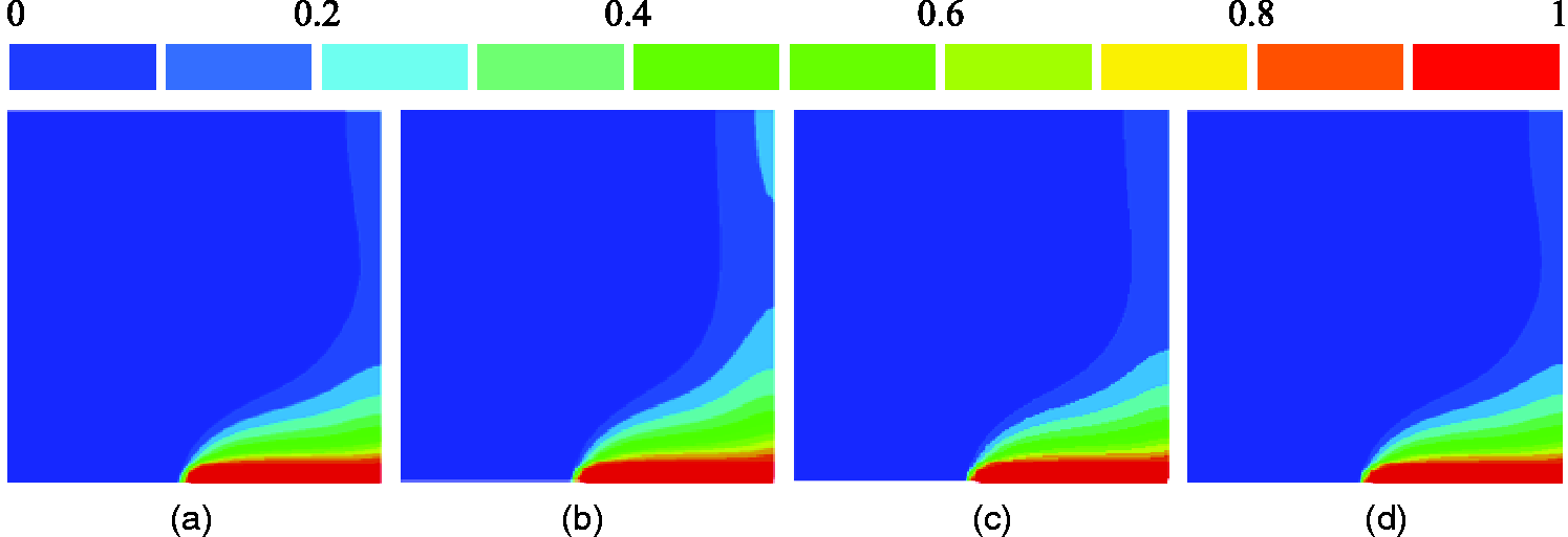
Damage profiles at $u = 0.006 d$ from (a) UEL reference solution, UMAT-UMATHT implementation with (b) c = 0.005, (c) c = 0.002 and (d) c = 0.0005.

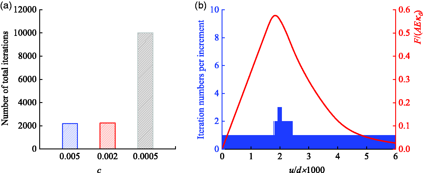
The UMAT-UMATHT approach, however, requires a smaller time step to ensure the stability of transient heat analysis. Abaqus determines the time increment according to the element size, heat velocity and the thermal parameters ( $ρ, c, k$ ). Referring to Figure 5(a) on the total number of iterations required to solve the same CTS problem with different values of c, we can infer that more computational resources is required with smaller c values. Hence, a general balance between the accuracy (compared to UEL reference solution) and computational time has to be made by the user.

Figure 5.

(a) Total number of iterations in UMAT-UMATHT with different c values, with 2500 CPE8T elements. For the same number of 8-noded elements, the UEL subroutine requires 42 iterations to solve the problem and (b) Number of iterations at each time increment using UMAT-UMATHT (c = 0.002) with 2500 elements, with the force-displacement graph superimposed. Note that the number of iterations corresponds to the global implicit scheme.

It is highlighted that the larger number of total iterations required in the UMAT-UMATHT implementation, is due to the smaller time steps, instead of the need for more iterations within a time step. To illustrate this, the problem is solved using 2500 CPE8T elements, c = 0.002, with a fixed time step. The number of iterations per time increment is depicted in Figure 5(b). It is easily observed that the solution at each time increment typically converges within one iterative step. This is in contrast to the numerical solution of a typical phase field damage model, where the non-convex potential energy function with respect to the field variables typically induces convergence issues with the standard Newton’s method. For example, similar tensile problems solved using different phase field damage models in Wu and Huang (2020); Navidtehrani et al. (2021) are shown to require a large number of iterations per increment, especially at the initial part of strain softening. Therewith, it was found that the quasi-Newton method is more robust for the implementation of phase field damage models (Kristensen and Martínez-Pañeda, 2020; Wu et al., 2020), but unfortunately, is not available in Abaqus for use with its in-built coupled temperature-displacement elements. We note that this numerical convergence issue is not encountered with the localizing gradient enhancement.

It is also highlighted that the visualization and post-processing of simulation results, using the Abaqus in-built elements for thermo-mechanical analyses, can be done easily with Abaqus/Viewer. In contrast, these tasks cannot be done directly when the UEL subroutine is used. Instead, additional efforts are required to establish a workaround, e.g. to include a dummy mesh of standard elements overlaying the user elements, or to regenerate an odb file by transferring the relevant output to the standard element mesh.

Finally, a customary check for mesh convergence is done using CPE3T triangular elements (linear displacement and linear $\tilde{e}$ ). We deliberately adopt a different element type here, compared to the earlier results, to further demonstrate the ease of implementation with UMAT-UMATHT.² As the change in element type (and shape functions) are accounted internally for by Abaqus, the same UMAT-UMATHT subroutines that were utilized earlier can be used here as well. The force-displacement graphs with different number of elements are shown in Figure 3(b), where mesh convergence is demonstrated.

Numerical examples considering other Abaqus in-built features

In this section, the UMAT-UMATHT implementation is adopted for more complex problems, involving the use of other in-built features in Abaqus. For the following examples, a conservative value of c = 0.0005 is adopted.

Example incorporating element deletion

To capture structural failure process, highly damaged elements can be removed via the deletion option in Abaqus. This feature is useful in cases with complex crack paths, or in situations with element distortions at large deformation. In this section, the damage variable ω is utilized as the user specified material state variable which controls the element deletion flag. A material point having a damage value beyond a threshold limit will be marked as deleted. An element will be removed from the mesh when all of its underlying material points are marked as deleted.

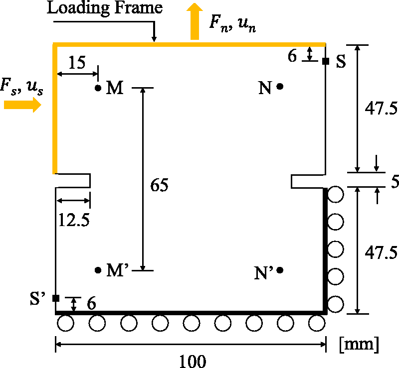
Here, we will demonstrate the use of this element deletion feature together with the localizing gradient enhancement, by considering the mixed mode fracture of a Double-Edge-Notched (DEN) specimen as reported in Nooru-Mohamed (1992). The DEN specimen with dimension of $100 mm \times 100 mm \times 50 mm$ (denoted as DEN100 hereafter) is illustrated in Figure 6. The loading path 6a (u_n = u_s) is considered, where u_n donates the average relative vertical displacement between points M-M′ and N-N′, and u_s indicating the relative lateral deformation between points S-S′.

Figure 6.

Geometry and boundary conditions of DEN100, where a proportional loading of u_n = u_s is applied to the loading frame (Nooru-Mohamed 1992).

The problem is solved using CPS8T elements (8-node plane stress element with biquadratic displacement and bilinear $\tilde{e}$ ), with very fine mesh size of 0.3 mm at the critical regions along the crack propagation path, as illustrated in Figure 7(a). The experimentally determined mechanical properties for DEM specimens: $E = 30 GPa$ and $ν = 0.2$ , are directly adopted to our model. Other numerical parameters are calibrated as k = 15.05, $l = 2 mm, κ_{0} = 9.8 \times 10^{- 5}$ and $β = 0.01$ . A material point is flagged as being deleted once $ω > 0.99$ . With these settings, the structural response is depicted in Figure 7(b), which matches well with the experimental data. The eroded elements, corresponding to the crack profiles at the final loading step in Figure 7(b), is depicted in Figure 8(a), which match well with the experimental observations (see Figure 8(b)). This demonstrates the viability of the element deletion option to be used in combination with the localizing gradient enhancement.

Figure 7.

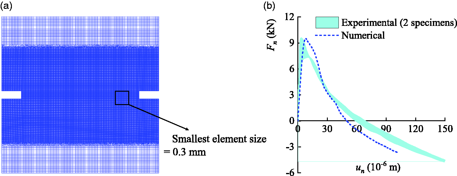
(a) FE discretization of DEN100 and (b) Numerical structural response compared against experimental data in Nooru-Mohamed (1992).

Figure 8.

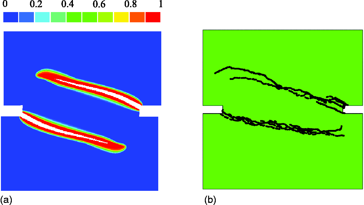
(a) Crack (eroded elements) patterns of DEN100 using localizing gradient enhancement (a magnification factor of 20 is utilized), with element deletion at $ω > 0.99$ and (b) Crack paths of DEN100 observed in the experiment (Nooru-Mohamed 1992).

Example incorporating contact between surfaces

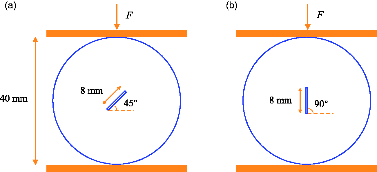
In this section, we refer to the compressive tests of 3D printed rock-like specimens with pre-existing flaws, as reported in Sharafisafa et al. (2018). Each specimen is placed between a pair of loading platens, and subjected to a displacement controlled applied force at 4 µm/s. Here, we consider single-flawed specimens with two different inclination angles ( $α = 45 °$ and $90 °$ ). Each disc has an in plane diameter of 40 mm and a thickness of 15 mm, as well as a pre-existing flaw of $8 mm \times 0.6 mm$ . The geometrical details are depicted in Figure 9. More information on the experimental set up can be found in Sharafisafa et al. (2018, 2019); Aliabadian et al. (2021).

Figure 9.

Geometry details for the compressive test of a rock-like specimen, with the pre-existing flaw orientating at (a) $α = 45 °$ and (b) $α = 90 °$ .

The following mechanical properties: $E = 1.35 GPa$ and $ν = 0.285$ , are experimentally determined for the 3D printed material, and are adopted in the numerical analyses. The length scale parameter is assumed as $l = 0.5 mm$ . Damage related parameters of k = 10, $κ_{0} = 1.75 \times 10^{- 3}$ and β = 7, are calibrated.

The specimen is meshed using CPS8T plane stress elements (8-node element with biquadratic displacement and bilinear $\tilde{e}$ ). Since the steel platens are much stiffer than the specimen, each of them is modelled as a 2-node rigid link (R2D2). At the interface between specimen and platen, the Abaqus feature of hard contact in normal behavior is selected. To prevent disc rotation, the top-most and bottom-most nodes of the specimen are constrained horizontally.

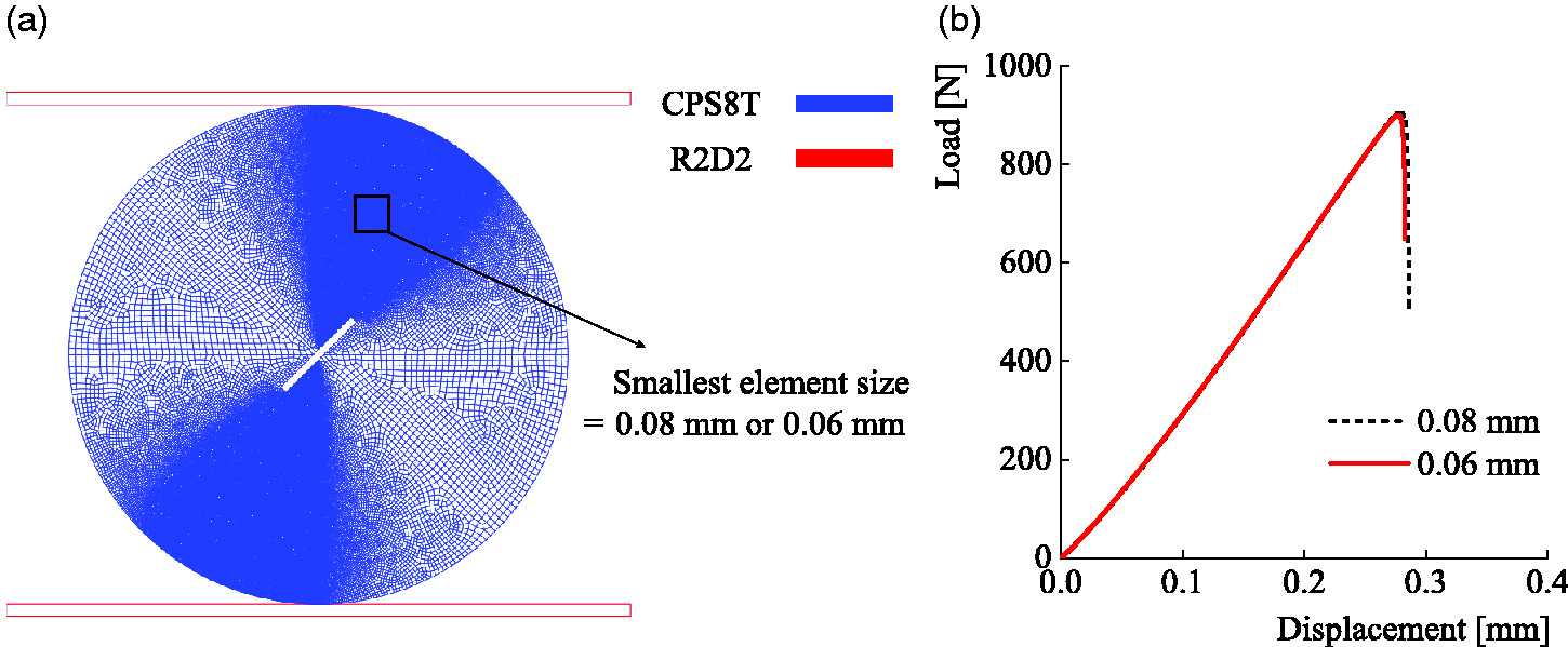
A mesh convergence check is first carried out for the specimen with $α = 45 °$ considering element sizes of 0.06 mm and 0.08 mm in the critical regions, as depicted in Figure 10(a). The structural responses in Figure 10(b) show that mesh convergence is achieved with element size of 0.08 mm. For the following analyses in this section, an element size of 0.08 mm will be used in the critical regions.

Figure 10.

(a) Meshing details and (b) mesh convergence for the specimen with $α = 45 °$ , with element sizes of 0.06 mm and 0.08 mm in the critical regions.

The structural responses of the single-flawed discs with $α = 45^{°}$ and $90^{°}$ are provided in Figure 11(a). Compared to the experimental data, the numerical results have higher elastic stiffness, and are more brittle. We note that Chen and Shen (2021), the same group that had conducted the experiment, has the same observations from their numerical simulations using smoothed particle hydrodynamics, as compared in Figure 11(a-i). It was postulated in Chen and Shen (2021) that the inconsistency may be due to the inadequacy of a 2D model in capturing the damage development/stiffness degradation along the thickness direction. Notwithstanding these differences, the peak forces obtained numerically match well with the experimental data for the two specimens. For each case, the fracture process initiates from the tips at both ends of the flaw, followed by an upward/downward propagation to the specimen surface, before the disc splits open in tension. This failure process is well captured by the localizing gradient damage model, as seen from the final damage profiles for both specimens in Figure 11(b), which compare well with the experimentally obtained digital image correlation (DIC) images in Figure 11(c).

Figure 11.

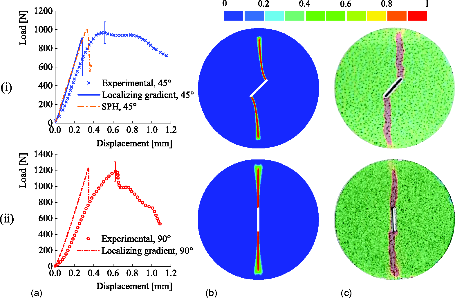
(a) Comparison between experimental data (Sharafisafa et al., 2018) and numerical structural responses obtained using localizing gradient enhancement, and smoothed particle hydrodynamics (Chen and Shen, 2021); failure patterns from (b) localizing gradient damage model and (c) experimental DIC images (Aliabadian et al., 2021), for the specimens with (i) $α = 45 °$ and (ii) $α = 90 °$ .

Example incorporating cohesive elements

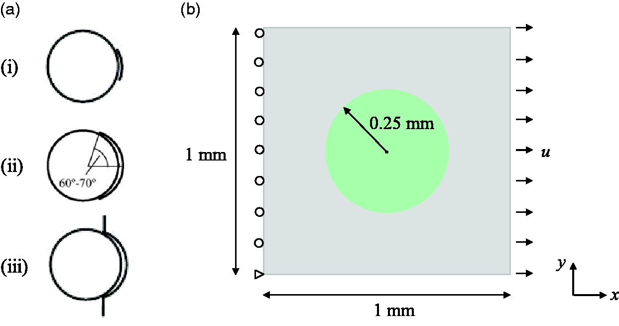
In this section, the meso-scale failure process of fiber-reinforced composites is considered. Referring specifically to carbon-epoxy systems, it was observed experimentally in París et al. (2007) that the failure process starts with the debonding of fiber-matrix interfaces at semi-angles of $60 ° - 70 °$ , leading to the initiation and propagation of macro cracks into the matrix. A schematic representation of the failure process is shown in Figure 12(a). In the literature, this failure process has been modelled with different numerical methods, e.g. discontinuous Galerkin/cohesive zone model (Nguyen, 2014), augmented Lagrangian functional cohesive zone model (Labanda et al., 2018) and coupled cohesive phase field model (Li et al., 2020).

Figure 12.

(a) Experimentally observed failure process of fiber-reinforced composites (París et al., 2007): (i) initial debonding of the fiber-matrix interface, (ii) debonding at semi-angles of $60 ° - 70 °$ and (iii) kinking of interface cracks into the matrix and (b) Geometry and boundary conditions of a single fiber embedded within matrix material.

In the following, we consider a unit cell comprising a single fiber embedded within the matrix material, with the unit cell subjected to a tensile load. This problem was solved in Nguyen et al. (2017) assuming plane stress condition, with the geometry and boundary conditions provided in Figure 12(b). Therewith, the fiber is elastic, and the matrix modelled using a kinematically enriched constitutive formulation that smeared a cohesive fracture over an element. At the fiber-matrix interface, cohesive elements following a bilinear traction-separation law are adopted.

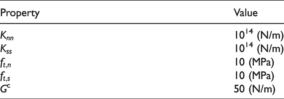
In our model, the Abaqus in-built cohesive elements are adopted to describe the fiber-matrix interfacial response. The fiber is elastic, and the matrix described using the localizing gradient damage model. Elastic properties of both materials are adopted from Nguyen et al. (2017), where $E_{f} = 40$ GPa, $ν_{f} = 0.33, E_{m} = 4$ GPa and $ν_{m} = 0.4$ . Additional parameters in the localizing gradient damage model are calibrated as $κ_{0} = 7.8 \times 10^{- 3}$ , l = 0.02 mm and $β = 0.01$ . Modelling parameters of interface are summarized in Table 2. Details on the traction-separation law adopted are provided in Appendix 2. The unit cell discretization is shown briefly in Figure 13, with 14693 CPS4T elements (4-node plane stress element with bilinear displacement and bilinear $\tilde{e}$ ) for the matrix material, 1296 CPS4 elements (4-node plane stress element with bilinear displacement) for the fiber, and 264 COH2D4 interface elements (4-node two-dimensional cohesive element) for the fiber-matrix interface.

Table 2.

Material properties of interface.

Property	Value
$K_{n n}$	10¹⁴ (N/m)
$K_{s s}$	10¹⁴ (N/m)
$f_{t, n}$	10 (MPa)
$f_{t, s}$	10 (MPa)
G ^c	50 (N/m)

Figure 13.

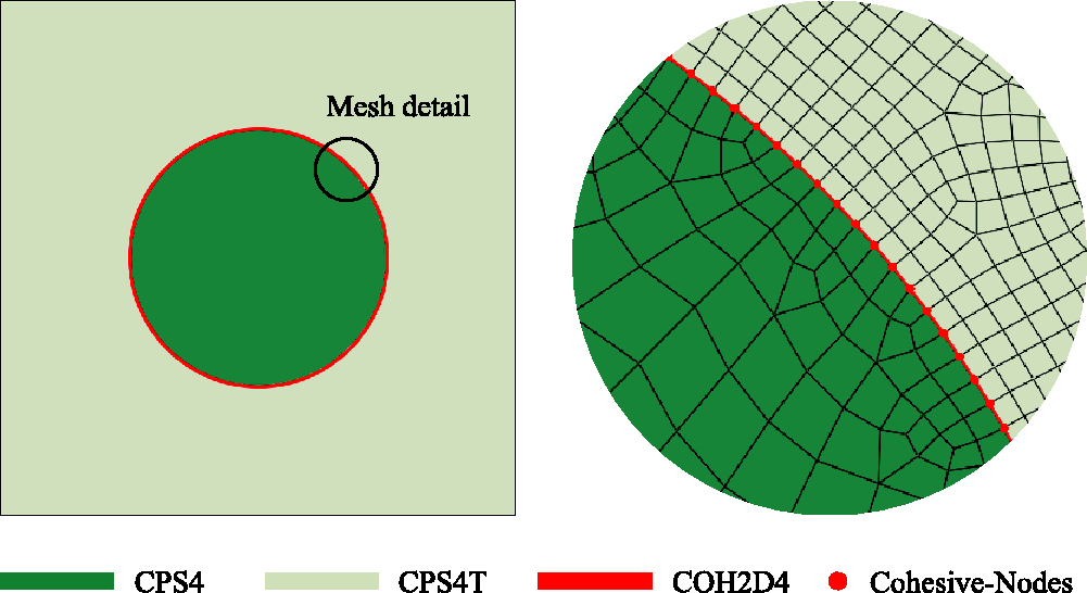
Mesh detail of the fiber-matrix composite: the matrix is discretized using CPS4 elements, the fiber discretized using CPS4T elements, and the interface discretized using COH2D4 interface elements.

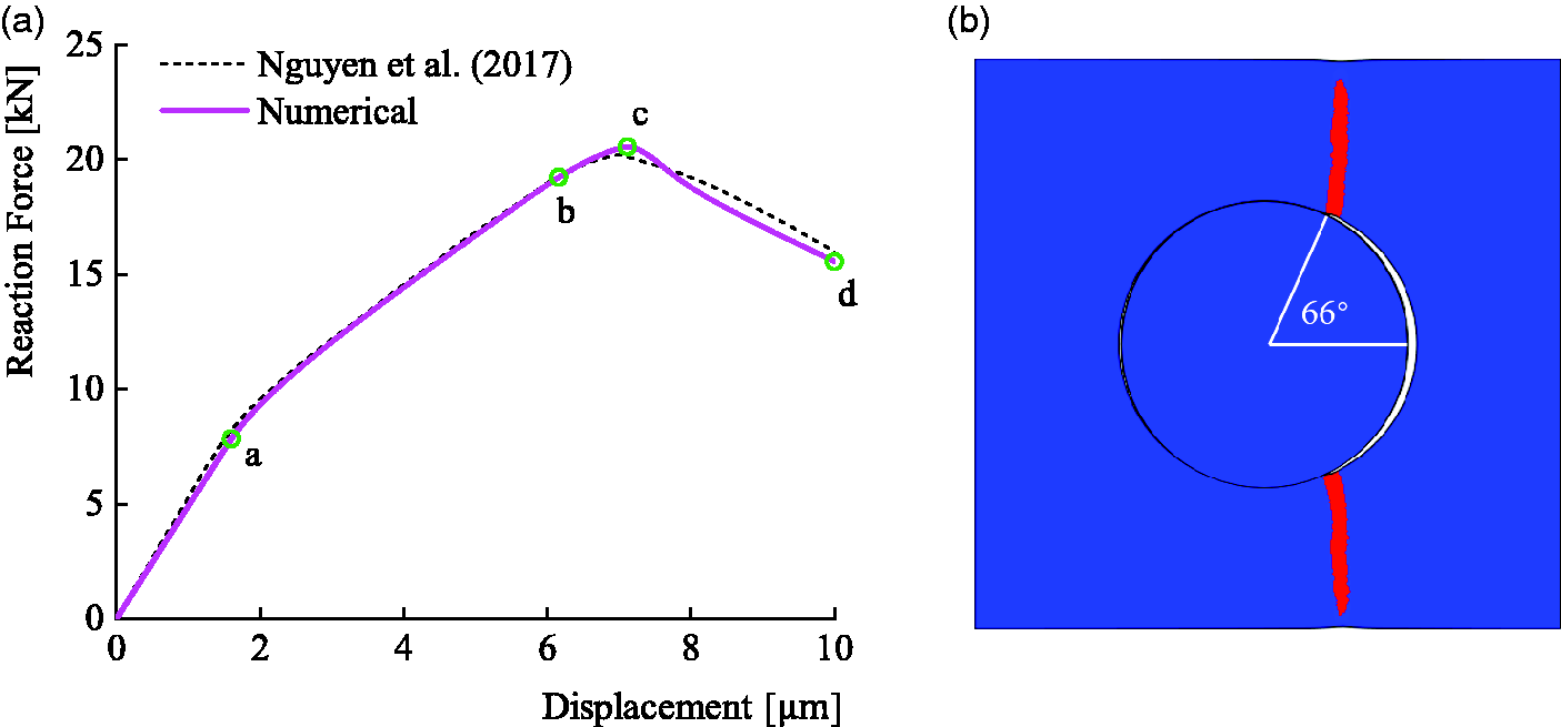
The reaction force versus displacement curve in Figure 14(a) shows a good agreement with the reference results from Nguyen et al. (2017). The failure pattern of the composite at $u = 10$ µm is provided in Figure 14(b), with the (damaged) cohesive elements removed from the deformed shape for better visualizing of the debonding phenomenon. The general failure process is captured correctly, with a kinked crack initiating from the interfacial crack and propagating into the matrix. The semi-debonding angle of $66^{°}$ obtained numerically is also within the range of $60 ° - 70 °$ suggested in París et al. (2007).

Figure 14.

(a) Numerical structural response compared to reference results and (b) Interfacial crack and damage ( $ω > 0.95$ ) propagation in the matrix material, at $u = 10$ µm (a magnification factor of 2 is utilized).

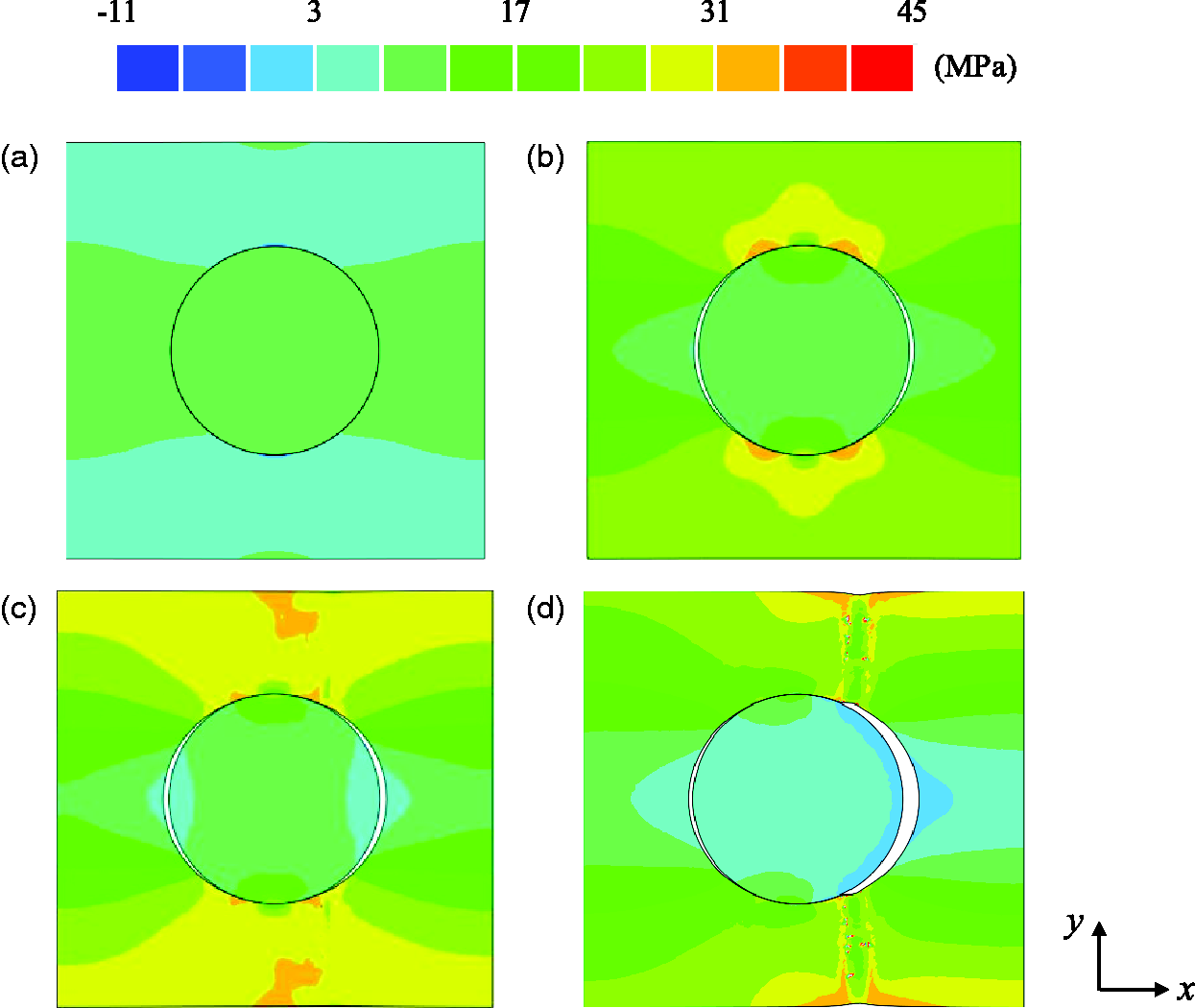
To better illustrate the failure process, the evolution of stress component along $x -$ axis is plotted in Figure 15, corresponding to the loading steps indicated in Figure 14. The fracture development at each loading step is briefly described as follows:

Figure 15.

Profiles of the stress component along $x -$ axis for the fiber-matrix composite, corresponding to the four loading stages (a)–(d) of Figure 14. A magnification factor of 5 is utilized.

Step a: The start of a nonlinear response. The failure process is expected to first initiate and propagate at the fiber-matrix interface, according to the stress distribution in Figure 15(a).

Step b: Debonded surfaces of matrix and fiber are created, with kinks developing at the tips of cohesive cracks.

Step c: Interfacial debonding continues. One of the kinks starts to dominate the failure process (here, the one on the right), with the crack starting to extend into the matrix material.

Step d: The kinked crack at the cohesive crack tip propagates upwards/downwards through the matrix material.

3D modelling of prismatic skew edge notched beam in torsion

The prevention of failure behavior in quasi-brittle materials is a major concern in the engineering field. Numerically, whenever appropriate, quasi-brittle fracture problems are modelled and solved either in 1D or 2D, to reduce computational cost. In many cases, however, the loading conditions may induce complex damage evolution processes to give non-planar crack surfaces and twisted crack trajectories. These problems require the use of a 3D model. This motivates the current section, where the localizing gradient damage model is employed for the 3D mixed mode fracture, by taking advantage of the simplified implementation approach. From the UMAT-UMATHT (2D) subroutines, the extension to 3D requires only the revision of mechanical constitutive laws, as well as the sensitivity terms with respect to the field variables.

3D implementation of localizing gradient damage model

In this section, an extension of the gradient enhancement from 2D to 3D is considered. The same notations and definitions of the UMAT-UMATHT variables follow those of Section ‘Numerical implementation in Abaqus’. Modifications required in the subroutines for 3D implementation are highlighted below.

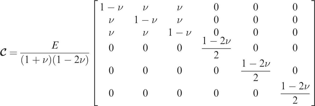
Focusing first on the mechanical constitutive behavior defined in UMAT, the stress and strain tensors have six components for 3D problems in Voigt notation. According to the element types adopted, the change in dimensions of stress and strain arrays is also accounted for internally by Abaqus. Thus, the stress constitutive law and the corresponding sensitivities with respect to the field variables, which were defined earlier in 2D, can be utilized for 3D implementation by redefining the elastic stiffness matrix, such that

STRESS \overset{def}{=} σ = (1 - ω) C : ε

(30a)

DDSDDE \overset{def}{=} \frac{d σ}{d ε} = (1 - ω) C

(30b)

DDSDDT \overset{def}{=} \frac{d σ}{d \tilde{e}} = - \frac{\partial ω}{\partial κ} C : ε

(30c)

where

C = \frac{E}{(1 + ν) (1 - 2 ν)} [\begin{matrix} 1 - ν & ν & ν & 0 & 0 & 0 \\ ν & 1 - ν & ν & 0 & 0 & 0 \\ ν & ν & 1 - ν & 0 & 0 & 0 \\ 0 & 0 & 0 & \frac{1 - 2 ν}{2} & 0 & 0 \\ 0 & 0 & 0 & 0 & \frac{1 - 2 ν}{2} & 0 \\ 0 & 0 & 0 & 0 & 0 & \frac{1 - 2 ν}{2} \end{matrix}]

Further, the mechanical heat generation RPL and the corresponding tangent contribution with respect to the strain field should be revised accordingly, i.e.

RPL \overset{def}{=} r_{pl} = e - \tilde{e}

(31a)

DRPLDE \overset{def}{=} \frac{d r_{pl}}{d ε} = \frac{\partial e}{\partial ε}

(31b)

where the equivalent strain measure e in equation (10) should be computed based on 3D condition.

Note that the UMATHT subroutine, which defines the constitutive thermal behavior, can be adopted directly for 3D analyses without any modifications.

Experimental setup and observations

We consider the prismatic skew edge notched beam with square cross section, as reported in Jefferson et al. (2004). Geometry details are depicted in Figure 16. In the experiment, the horizontally positioned plane concrete beam is clamped with collars at both ends. Three of the four steel arms are constrained in the vertical direction, while the last one is subjected to a downward concentrated load. The clamping frames are designed to make perfect contact with the concrete specimen to ensure transferring of the eccentric load to the specimen, which leads to a torsional moment aligned with the axis of the beam. Figure 17(a) illustrates the final damage of the prismatic beam under the torsional loading, where a complex fracture behavior is observed. The fracture surfaces are spatially twisted and warped, which initiate from the notch front and intersect the bottom surfaces with a kind of S-shaped curve.

Figure 16.

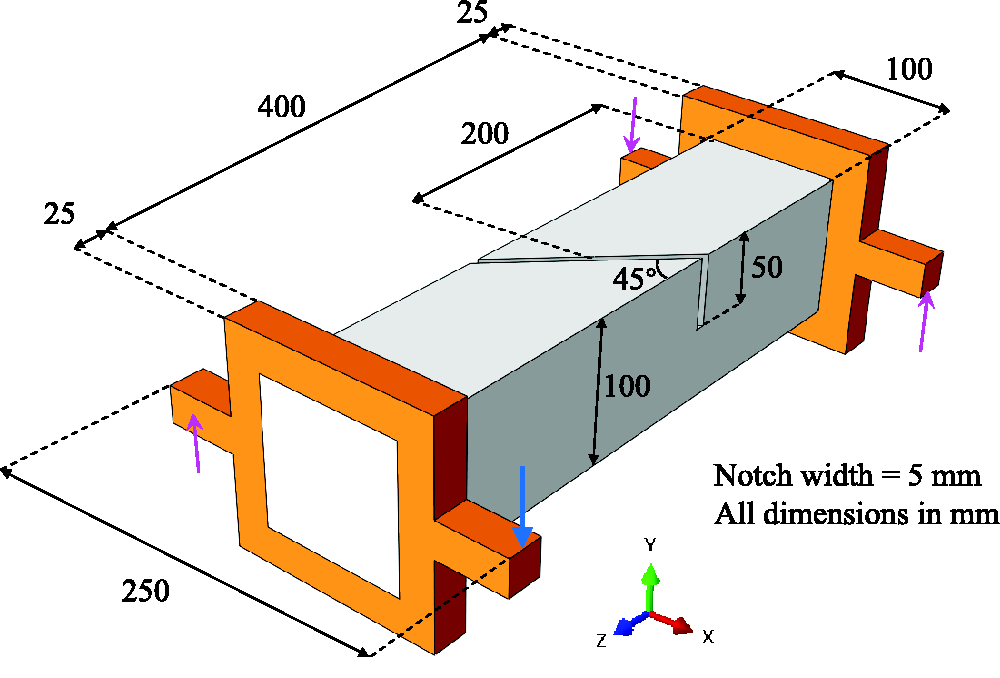
Geometry and boundary conditions for the notched prismatic torsion test (Jefferson et al., 2004).

Figure 17.

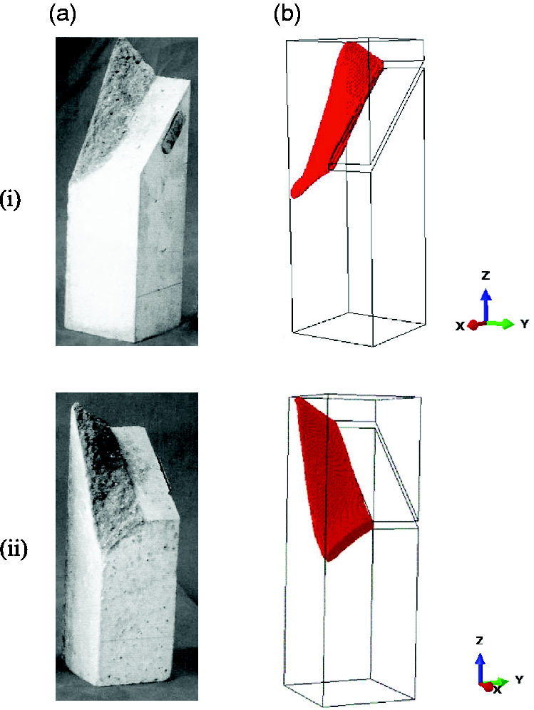
Comparison of the fracture surfaces for the notched prismatic concrete beam under torsional loading between (a) experimental observations (Jefferson et al., 2004) and (b) numerical results using localizing gradient damage enhancement (considered as $ω > 0.95$ ), from different views of (i) and (ii).

Numerical results and discussions

Due to the complex fracture surface that wraps around the beam’s longitudinal axis, the problem has to be solved in 3D. To apply the torsional loading, one of the right steel arms is vertically supported in the middle, the left two arms are fixed at a single point. A downward displacement u is imposed on the last steel arm, as depicted in Figure 18. The CMOD is defined as norm of the relative distances between points A and B along x and z directions. To reduce computational cost, only the critical region highlighted in Figure 18 is modelled using the localizing gradient enhancement. The standard elastic model is adopted for the remaining parts of the specimen, as well as the steel collars. 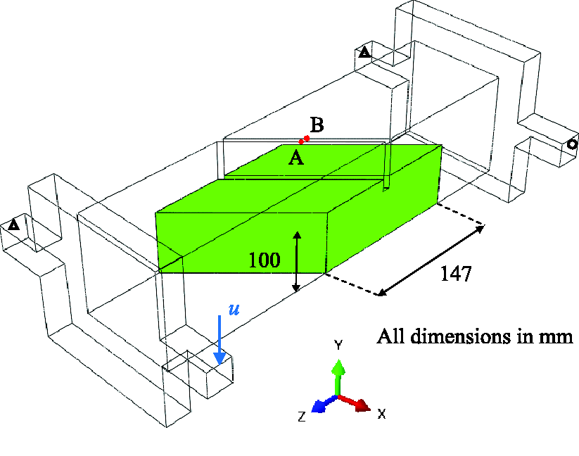The experimentally obtained mechanical properties for concrete, $E = 35 GPa$ and $ν = 0.2$ are adopted. The damage related parameters, i.e. k = 10, $κ_{0} = 7.2 \times 10^{- 3}$ , l = 1 mm and β = 120, are calibrated accordingly. A detailed discussion on the influence of the parameter c in equation (20) can be found in Section ‘Plane strain analysis’. Here, c = 0.002 is utilized.

Figure 18.

Boundary conditions and critical damage region in the numerical simulation for the prismatic skew edge notched beam under torsional loading.

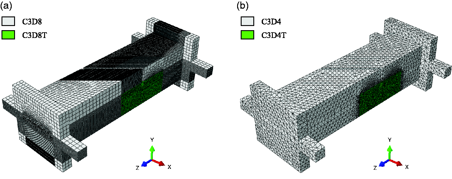
Considering two different discretization methods, the specimen is meshed using:

462580 C3D8T elements (8-node brick element with trilinear displacement and $\tilde{e}$ ) and 268200 C3D8 elements (8-node brick element with trilinear displacement), as depicted in Figure 19(a);

Figure 19.

Mesh details of the prismatic skew edge notched beam: (a) the critical damage region is discretized using C3D8T elements, the remaining parts discretized using C3D8 elements and (b) the critical damage region is discretized using C3D4T elements, the remaining parts discretized using C3D4 elements.

2646554 C3D4T elements (4-node tetrahedron element with linear displacement and $\tilde{e}$ ) and 709144 C3D4 elements (4-node tetrahedron element with linear displacement), as depicted in Figure 19(b).

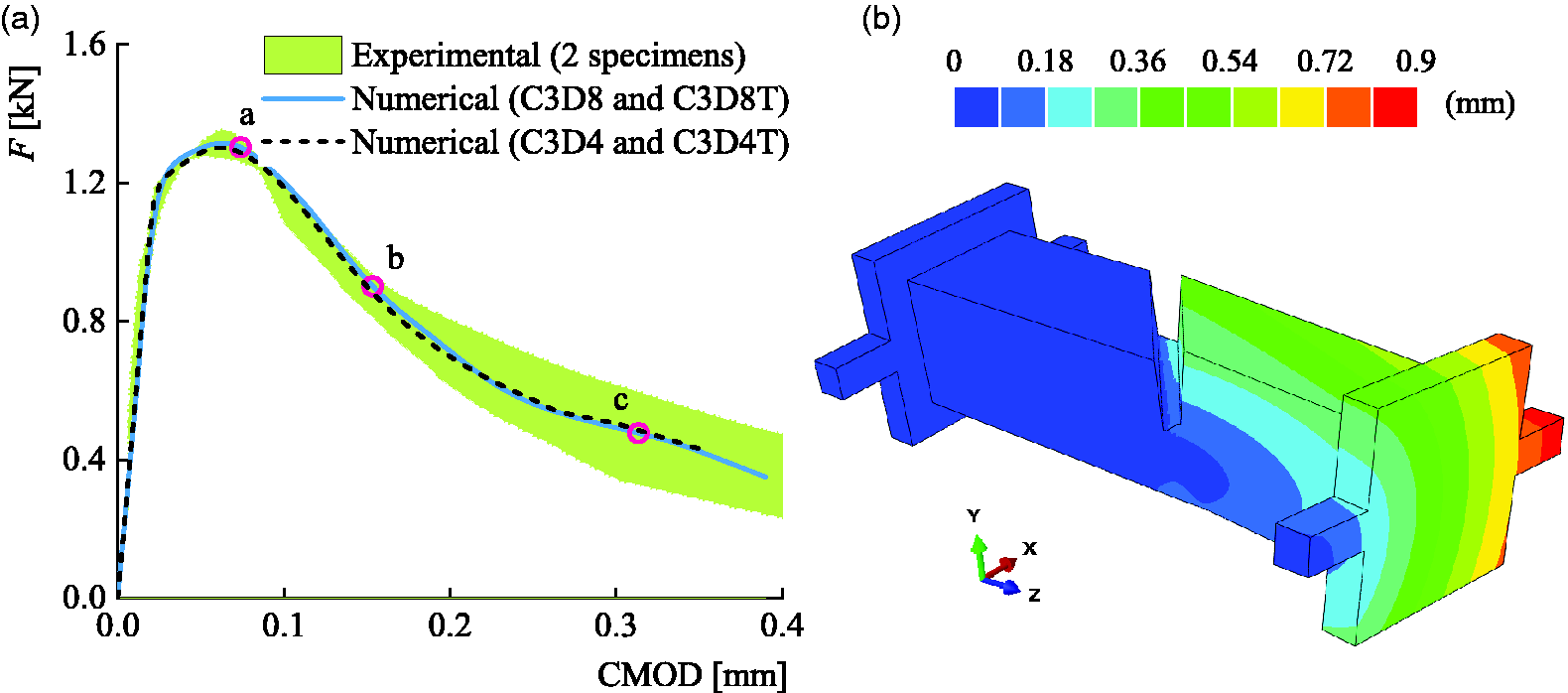
A converged structural response is obtained (see Figure 20(a)). It is shown that the reaction force versus CMOD curve matches well with the two sets of experimental data. The displacement magnitude ( $\sqrt{u_{x}^{2} + u_{y}^{2} + u_{z}^{2}}$ ) of the specimen, corresponding to the final loading step indicated in Figure 20(a), is visualized in Figure 20(b), where the twisting of the concrete beam around z-axis is clearly observed, together with the relative opening and sliding of both notch edges.

Figure 20.

(a) Comparison between experimental data (Jefferson et al., 2004) and numerical results with two different mesh types using the localizing gradient damage model for the prismatic skew edge notched beam and (b) Profiles of the displacement magnitude for the prismatic skew edge notched beam under torsional loading, corresponding to Step c. A magnification factor of 50 is adopted.

The crack profiles obtained using the localizing gradient damage model are compared against the experimental results of Jefferson et al. (2004), as depicted in Figure 17. For ease of visualization, elements with damage $ω \leq 0.95$ are removed, to reveal the fracture surface. As discussed, the numerical spatially distorted fracture surfaces and curved crack paths are very similar to the experimental results.

Finally, fracture evolution of the specimen corresponding to different loading stages of Figure 20 is examined in Figure 21. The results match well with the experimental descriptions, in which a localized damage band initiates from the bottom edges of the notch, before propagating with a rotational effect to intersect with the base to form a S-curve.

Figure 21.

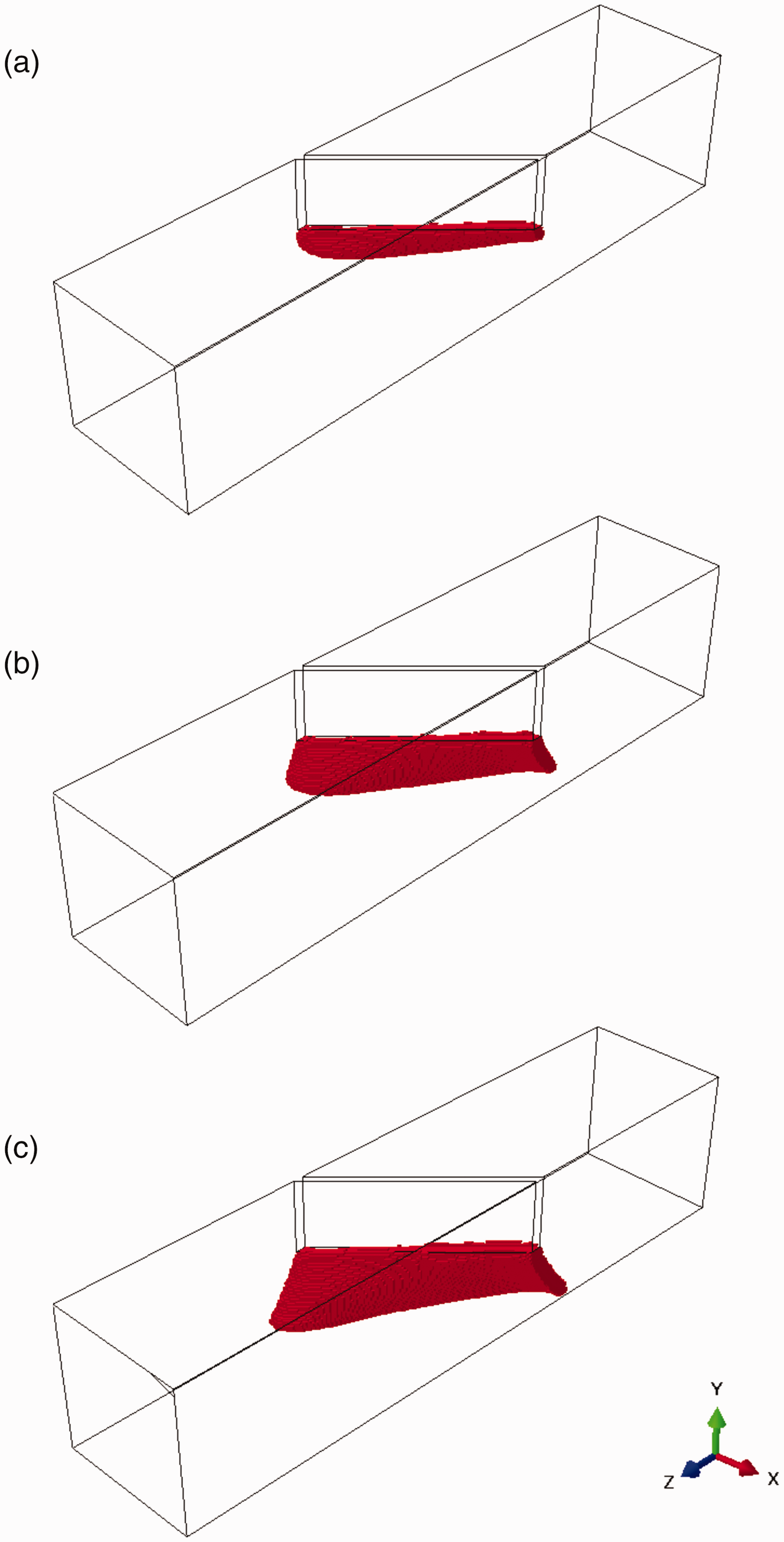
The growth of crack (considered as $ω > 0.95$ ) in the prismatic skew edge notched beam, corresponding to the three loading stages (a)-(c) indicated in Figure 20.

Conclusion

In this contribution, a simple implementation approach of the localizing gradient damage model in the commercial FE software Abaqus is presented, by utilizing its in-built coupled temperature-displacement elements. The balance equation governing the localizing gradient enhancement involves the divergence of a nonlinear flux term. Accordingly, the UMAT and UMATHT subroutines are adopted for defining the mechanical and thermal constitutive relations, as well as the associated sensitivities with respect to the field variables. With the proper definitions of material parameters, the temperature field can be made analogous to the nonlocal variable, such that the heat equation almost recovers the balance equation of the gradient enhanced model. Compared to the standard implementation method by writing a user element subroutine, this simplified approach is more manageable for an average user.

To recover the balance equation of the localizing gradient enhancement, the transient term in the heat equation described by UMATHT has to be set as small as possible. However, the time step required for numerical stability is dependent on the magnitude of this transient term. The conflicting requirements to closely approximate the gradient damage model and having lower computational time can be thus considered as a drawback. It is shown that convergence occurs rapidly within a time-step, which helps to mitigate the effect of small time steps. Moreover, the simplified implementation approach enables the direct visualization and post-processing of results in Abaqus/Viewer – a feature that is not possible with the standard implementation method via user element subroutine.

The versatility of the simplified implementation approach is demonstrated with the tensile loading of a compact tension specimen, solved using different element types. Additionally, it is shown that the localizing gradient damage model can be used in conjunction with other Abaqus features, e.g. element deletion, contact between surfaces and the incorporation of cohesive elements, with good numerical predictions obtained for the problems considered. Finally, it is demonstrated that the simplified implementation approach can be extended to 3D analyses easily. Considering the torsional loading of a prismatic concrete beam, the localizing gradient enhancement is shown to capture well the complex 3D twisting fracture behavior.

Footnotes

Declaration of conflicting interests

The author(s) declared no potential conflicts of interest with respect to the research, authorship, and/or publication of this article.

Funding

The author(s) received no financial support for the research, authorship, and/or publication of this article.

ORCID iDs

Yi Zhang

Leong Hien Poh

Notes

References

Ahmed

Voyiadjis

Park

(2021a) Local and non-local damage model with extended stress decomposition for concrete. International Journal of Damage Mechanics 30(8): 1149–1191.

Ahmed

Voyiadjis

Park

(2021b) A nonlocal damage model for concrete with three length scales. Computational Mechanics 68(3): 461–486.

Aliabadian

Sharafisafa

Tahmasebinia

, et al. (2021) Experimental and numerical investigations on crack development in 3D printed rock-like specimens with pre-existing flaws. Engineering Fracture Mechanics 241: 107396.

Azinpour

Ferreira

JPS

Parente

MPL

, et al. (2018) A simple and unified implementation of phase field and gradient damage models. Advanced Modeling and Simulation in Engineering Sciences 5(1): 1–24.

Castillo

Nguyen

Niiranen

(2021) Spatially random modulus and tensile strength: Contribution to variability of strain, damage, and fracture in concrete. International Journal of Damage Mechanics 30(10): 1497–1523.

Chen

Shen

(2021) A modified smoothed particle hydrodynamics for modelling fluid-fracture interaction at mesoscale. Computational Particle Mechanics 9(2): 277–297.

de Vree

Brekelmans

Van Gils

(1995) Comparison of nonlocal approaches in continuum damage mechanics. Computers & Structures 55(4): 581–588.

Geers

MGD

de Borst

Brekelmans

WAM

, et al. (1998) Strain-based transient-gradient damage model for failure analyses. Computer Methods in Applied Mechanics and Engineering 160(1–2): 133–153.

Giry

Dufour

Mazars

(2011) Stress-based nonlocal damage model. International Journal of Solids and Structures 48(25–26): 3431–3443.

10.

Grégoire

Rojas-Solano

Pijaudier-Cabot

(2013) Failure and size effect for notched and unnotched concrete beams. International Journal for Numerical and Analytical Methods in Geomechanics 37(10): 1434–1452.

11.

Havlásek

Grassl

Jirásek

(2016) Analysis of size effect on strength of quasi-brittle materials using integral-type nonlocal models. Engineering Fracture Mechanics 157: 72–85.

12.

Jefferson

Barr

BIG

Bennett

, et al. (2004) Three dimensional finite element simulations of fracture tests using the Craft concrete model. Computers and Concrete 1(3): 261–284.

13.

Jirásek

Desmorat

(2019) Localization analysis of nonlocal models with damage-dependent nonlocal interaction. International Journal of Solids and Structures 174-175: 1–17.

14.

Kristensen

Martínez-Pañeda

(2020) Phase field fracture modelling using quasi-Newton methods and a new adaptive step scheme. Theoretical and Applied Fracture Mechanics 107: 102446.

15.

Labanda

Giusti

Luccioni

(2018) Meso-Scale fracture simulation using an augmented Lagrangian approach. International Journal of Damage Mechanics 27(1): 138–175.

16.

Yin

Zhang

, et al. (2020) Modeling microfracture evolution in heterogeneous composites: a coupled cohesive phase-field model. Journal of the Mechanics and Physics of Solids 142: 103968.

17.

Marzec

Bobiński

(2019) On some problems in determining tensile parameters of concrete model from size effect tests. Polish Maritime Research 26(2): 115–125.

18.

Mobasher

Berger-Vergiat

Waisman

(2017) Non-local formulation for transport and damage in porous media. Computer Methods in Applied Mechanics and Engineering 324: 654–688.

19.

Navidtehrani

Betegón

Martínez-Pañeda

(2021) A simple and robust Abaqus implementation of the phase field fracture method. Applications in Engineering Science 6: 100050.

20.

Negi

Singh

Kumar

(2021) Structural size effect in concrete using a micromorphic stress-based localizing gradient damage model. Engineering Fracture Mechanics 243: 107511.

21.

Nguyen

(2011) A damage model with evolving nonlocal interactions. International Journal of Solids and Structures 48(10): 1544–1559.

22.

Nguyen

(2014) Discontinuous Galerkin/extrinsic cohesive zone modeling: Implementation caveats and applications in computational fracture mechanics. Engineering Fracture Mechanics 128: 37–68.

23.

Nguyen

, et al. (2017) Modelling complex cracks with finite elements: A kinematically enriched constitutive model. International Journal of Fracture 203(1-2): 21–39.

24.

Nooru-Mohamed MB (1992) Mixed-mode fracture of concrete: An experimental approach. PhD thesis, Delft University of Technology. Delft: The Netherlands.

25.

Ostwald

Kuhl

Menzel

(2019) On the implementation of finite deformation gradient-enhanced damage models. Computational Mechanics 64(3): 847–877.

26.

Papadioti

Aravas

Lian

, et al. (2019) A strain-gradient isotropic elastoplastic damage model with J³ dependence. International Journal of Solids and Structures 174: 98–127.

27.

París

Correa

Mantič

(2007) Kinking of transversal interface cracks between fiber and matrix. Journal of Applied Mechanics 74(4): 703–716.

28.

Peerlings

RHJ

de Borst

Brekelmans

WAM

, et al. (1996) Gradient enhanced damage for quasi-brittle materials. International Journal for Numerical Methods in Engineering 39(19): 3391–3403.

29.

Peerlings

RHJ

de Borst

Brekelmans

WAM

, et al. (1998) Gradient-enhanced damage modelling of concrete fracture. Mechanics of Cohesive-Frictional Materials 3(4): 323–342.,

30.

Peerlings

RHJ

Geers

MGD

de Borst

, et al. (2001) A critical comparison of nonlocal and gradient-enhanced softening continua. International Journal of Solids and Structures 38(44-45): 7723–7746.,

31.

Pereira

Weerheijm

Sluys

(2017) A numerical study on crack branching in quasi-brittle materials with a new effective rate-dependent nonlocal damage model. Engineering Fracture Mechanics 182: 689–707.

32.

Pijaudier-Cabot

Bažant

(1987) Nonlocal damage theory. Journal of Engineering Mechanics 113(10): 1512–1533.

33.

Poh

Sun

(2017) Localizing gradient damage model with decreasing interactions. International Journal for Numerical Methods in Engineering 110(6): 503–522.

34.

Roth

Hütter

Mühlich

, et al. (2012) Visualisation of user defined finite elements with ABAQUS/viewer. GACM Rep 5: 7–14.

35.

Sarkar

Singh

Mishra

(2020) A thermo-mechanical gradient enhanced damage method for fracture. Computational Mechanics 66(6): 1399–1426.

36.

Sarkar

Singh

Mishra

(2021) A simplified continuous–discontinuous approach to fracture based on decoupled localizing gradient damage method. Computer Methods in Applied Mechanics and Engineering 383: 113893.

37.

Sarkar

Singh

Mishra

, et al. (2019) A comparative study and ABAQUS implementation of conventional and localizing gradient enhanced damage models. Finite Elements in Analysis and Design 160: 1–31.

38.

Schreter

Neuner

Hofstetter

(2018) Evaluation of the implicit Gradient-Enhanced regularization of a damage-plasticity rock model. Applied Sciences 8(6): 1004.

39.

Seupel

Hütter

Kuna

(2018) An efficient FE-implementation of implicit gradient-enhanced damage models to simulate ductile failure. Engineering Fracture Mechanics 199: 41–60.

40.

Sharafisafa

Shen

(2018) Characterisation of mechanical behaviour of 3D printed rock-like material with digital image correlation. International Journal of Rock Mechanics and Mining Sciences 112: 122–138.

41.

Sharafisafa

Shen

Zheng

, et al. (2019) The effect of flaw filling material on the compressive behaviour of 3D printed rock-like discs. International Journal of Rock Mechanics and Mining Sciences 117: 105–117.

42.

Shedbale

Sun

Poh

(2021) A localizing gradient enhanced isotropic damage model with Ottosen equivalent strain for the mixed-mode fracture of concrete. International Journal of Mechanical Sciences 199: 106410.

43.

Simone

Askes

Sluys

(2004) Incorrect initiation and propagation of failure in non-local and gradient-enhanced media. International Journal of Solids and Structures 41(2): 351–363.

44.

Systèmes

(2014) Abaqus User Subroutines Reference Guide, Version 6.14. Providence, RI, USA: Dassault Systemes Simulia Corp..

45.

Tong

Hua

Liu

, et al. (2021a) Localizing gradient damage model coupled to extended microprestress-solidification theory for long-term nonlinear time-dependent behaviors of concrete structures. Mechanics of Materials 154: 103713.

46.

Tong

Yuan

Wang

, et al. (2021b) The role of bond strength in structural behaviors of UHPC-NC composite beams: Experimental investigation and finite element modeling. Composite Structures 255: 112914.

47.

Wang

Shedbale

Kumar

, et al. (2019) Localizing gradient damage model with micro inertia effect for dynamic fracture. Computer Methods in Applied Mechanics and Engineering 355: 492–512.

48.

Wosatko

Pamin

Winnicki

(2018) Numerical prediction of deterministic size effect in concrete bars and beams. In: Computational modelling of concrete structures: Proceedings of the conference on computational modelling of concrete and concrete structures (EURO-C 2018), Bad Hofgastein, Austria. New York: CRC Press, pp.447–456.

49.

Huang

(2020) Comprehensive implementations of phase-field damage models in Abaqus. Theoretical and Applied Fracture Mechanics 106: 102440.

50.

Huang

Nguyen

(2020) On the BFGS monolithic algorithm for the unified phase field damage theory. Computer Methods in Applied Mechanics and Engineering 360: 112704.

51.

Biswas

Poh

(2020) Modelling of localized ductile fracture with volumetric locking-free tetrahedral elements. International Journal for Numerical Methods in Engineering 121(12): 2626–2654.

52.

Poh

(2019) Localizing gradient-enhanced Rousselier model for ductile fracture. International Journal for Numerical Methods in Engineering 119(9): 826–851.

53.

Zhang

Shedbale

Gan

, et al. (2021) Size effect analysis of quasi-brittle fracture with localizing gradient damage model. International Journal of Damage Mechanics 30(7): 1012–1035.

54.

Zreid

Kaliske

(2018) A gradient enhanced plasticity–damage microplane model for concrete. Computational Mechanics 62(5): 1239–1257.