Use of fabric tensors in damage and healing mechanics of materials

Abstract

A mathematical formulation incorporating the relationship between the damage tensor, healing tensor, and fabric tensors is presented. This formulation provides for a direct link between the subjects of Damage and Healing Mechanics using Fabric Tensors. A new damage-healing tensor is introduced that is based on the fabric of the material. This new tensor is pivotal in characterizing the micro-structure of the material, especially the distributions of micro-cracks and other micro defects. It is noted that the theory applies to linear elastic materials but can be generalized to other constitutive models incorporating inelastic behavior. As examples, the authors solve three cases, namely those of plane stress, plane strain, and isotropic elasticity. The case of plane stress assumes plane damage and plane healing as will be illustrated in the equations. Similarly, the case of plane strain is also illustrated. The case of isotropic elasticity assumes the presence of isotropic damage and isotropic healing. As an illustration, a numerical example is shown for a certain micro-crack distribution. Finally, experimental results are shown to illustrate the relationship between the fabric tensor parameters and the components of the damage and healing tensors. Finally, the evolution of damage and healing are discussed based on sound thermodynamic principles.

Keywords

Damage mechanics experimental characterization of fabric fabric tensors healing mechanics micro-cracks micro-structure thermodynamic principles

Introduction

The aim of this work is to present new damage-healing tensors that rely on the micro-structure of the material. The topic of continuum damage mechanics relies heavily on the introduction of a suitable damage tensor or damage variable. The aim here is to try to develop a link between the damage tensor/healing tensor with the those of fabric tensors which are physical based. Fabric tensors have been derived initially by Kanatani (1984a) to characterize the micro-mechanics of the material in terms of micro-cracks and other defects. This subject has been further advanced by the work of Lubarda and Krajcinovic (1993).

The subject of fabric tensors has been applied to rock materials by Satake (1982). In this way, it was generally applied to granular materials. The anisotropy of the distribution due to the fabric is represented by a mathematical tensor in terms of the normal vectors to the cracks (Kanatani, 1984a; Satake, 1982). There is a direct mathematical relationship between the fabric tensor and the probability distribution of the various existing micro-cracks.

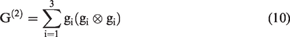
Fabric tensors have been derived mathematically and systematically by Kanatani (1984a, 1984b). He developed three types of fabric tensors: fabric tensors of the first kind, named $N$ , fabric tensors of the second kind, named $F$ , and fabric tensors of the third kind, named $D$ . He showed and presented the precise mathematical relationships between these three types of fabric tensors. These relationships are shown here in detail.

The application of fabric tensors to micro-structural distributions of micro-cracks was performed in detail by Lubarda and Krajcinovic (1993). These researchers studied the relations between a certain distribution of micro-cracks and the various types of fabric tensors. They used this information to plot a rose diagram or also called a circular histogram for the studied micro-crack distribution. This issue is illustrated here also in detail.

Isotropic damage mechanics has advanced quickly during the past decades. This subject relies on the use of a scalar damage variable in order to characterize the damage process, which is assumed to be isotropic. Cauvin and Testa (1999) that two independent damage variables should be used in order to characterize correctly isotropic damage. Other researchers who worked in this filed are Lemaitre, (Lemaitre, 1984) and Hayhurst and others (Chow and Wang, 1987a; Hayhurst, 1972; Lee et al., 1985). This has led other scientists to study the case of anisotropic damage. This most general theory of anisotropic damage was studied extensively by these researchers (Cordebois, 1983; Cordebois and Sidoroff, 1979; Sidoroff 1981) and later used by Lee et al. (1985) and Chow and Wang (1987b, 1988) to solve simple ductile fracture problems. Others who worked on this topic include Krajcinovic and Fonseka (1981), Murakami and Ohno (1981), Murakami (1983), and Krajcinovic (1983). Krempl (1981) also investigated this subject. In addition, the authors Voyiadjis and Kattan (1992, 1999) used continuum damage mechanics to advance further this subject and apply its principles to other materials (Kattan and Voyiadjis, 1990, 1993, 2001a, 2001b; Voyiadjis and Kattan, 1990, 1992, 1996, 1999; Voyiadjis and Park, 1997, 1999).

The mathematics of anisotropic damage mechanics and the tensorial nature of the damage variable, i.e. the damage tensor, have been developed by several researchers (Leckie and Onat, 1981; Murakami and Ohno, 1981). See also the references by (Onat, 1986; Onat and Leckie, 1988). Betten (1981, 1986) also studied the damage tensor extensively with great mathematical and systematic inquiry.

Figure 1 includes a flowchart that shows the precise steps to be used in order to solve a practical engineering application. In addition, Figure 2 includes a random and specific micro-crack distribution shown here for illustration purposes only. The author previously developed the relations between the damage tensor and fabric tensors but without including healing effects (Voyiadjis and Kattan, 2006a). They also elaborated further on this relationship with subsequent work (Voyiadjis and Kattan, 2006b). Further work by the authors can also be cited (Voyiadjis and Kattan, 2007a, 2007b; Krajcinovic 1983 and Krajcinovic 1996).

Figure 1.

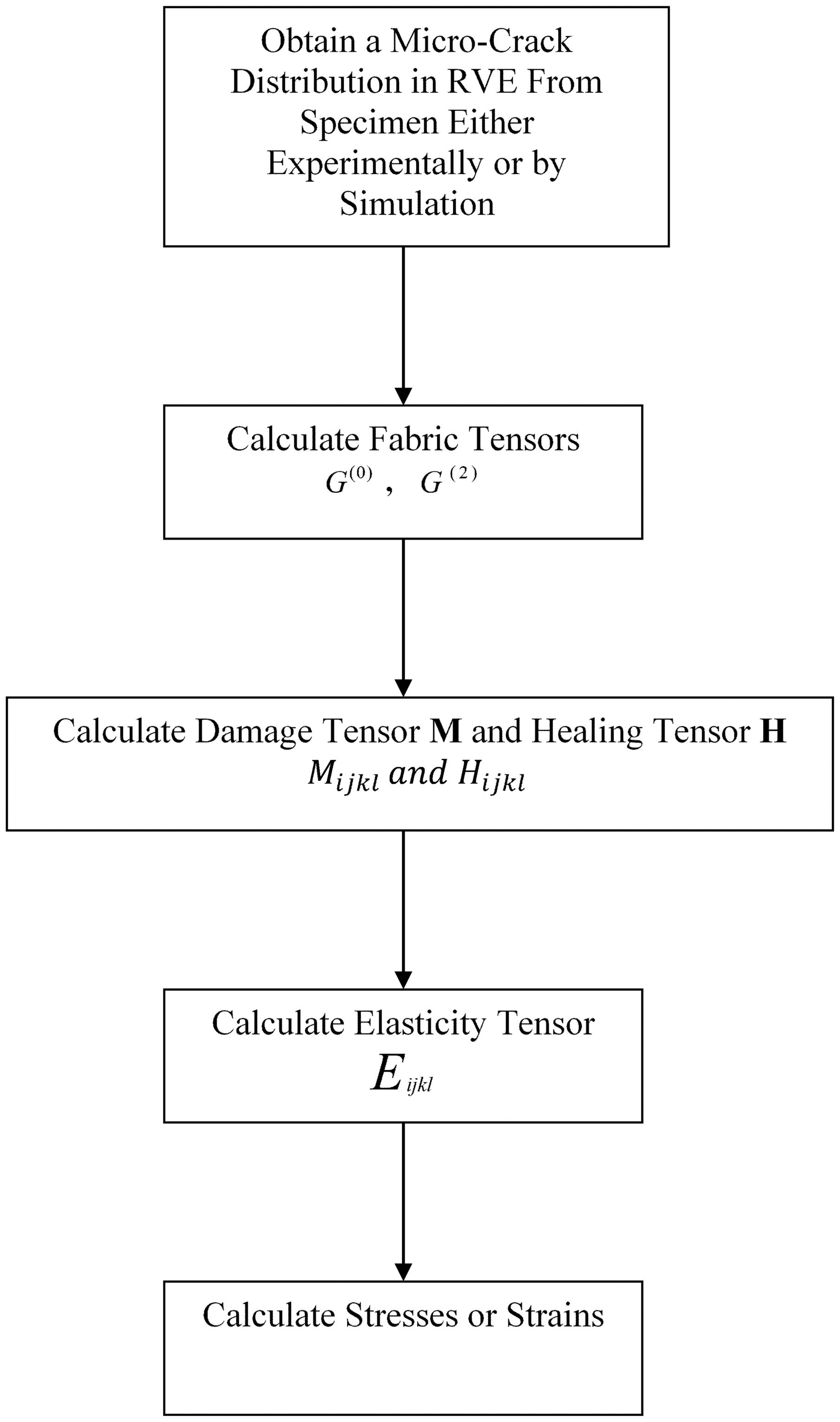
Illustration of the steps to solve a problem with a micro-crack distribution.

Figure 2.

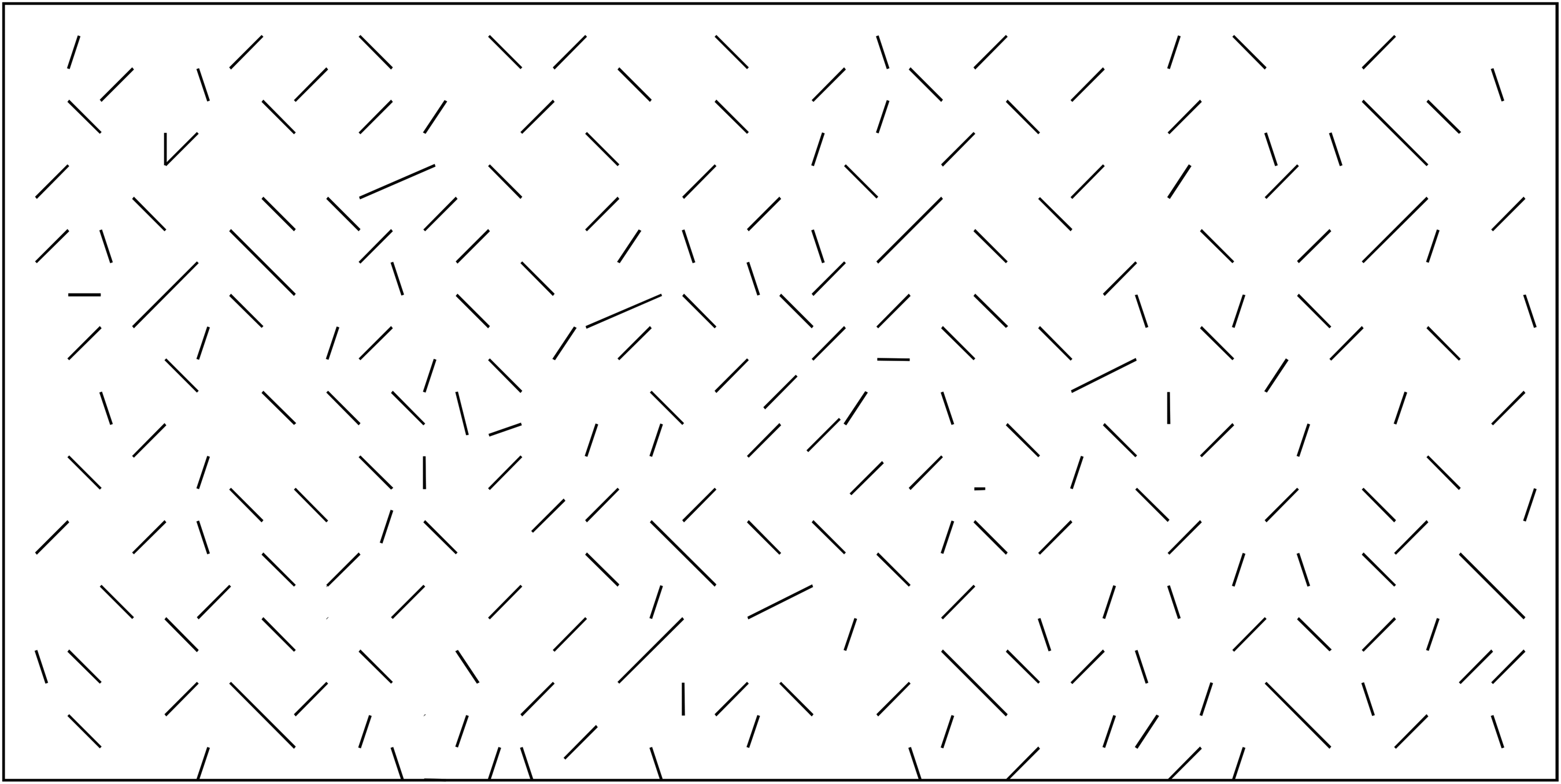
An example of a micro-crack distribution.

In this regard, the new topic of healing mechanics is introduced and used to derive new damage and healing tensors that are based on fabric tensors. These tensors are derived mathematically and systematically. One first starts with the formula of the elasticity tensor written in terms of fabric tensors that is available in the literature (Voyiadjis and Kattan, 2006a, 2006b). Then one uses the relationship between the elasticity tensor and the damage and healing tensors to produce a valid relationship between fabric tensors on the one hand and damage and healing tensors on the other hand. This relationship is derived twice – once for the hypothesis of strain equivalence and another time for the hypothesis of elastic energy equivalence. It is seen that the relationship for strain equivalence is much simpler and more direct than the other one for elastic energy equivalence.

Note that the formulation is presented for linear elastic materials. In the general formulation, the most general case of anisotropic elasticity with anisotropic damage and anisotropic healing is considered. Three examples are solved – the first one is plane stress with plane damage and plane healing. The second one is plane strain with plane damage and plane healing. The third one is more rigorous and involves the three-dimensional case of isotropic elasticity with isotropic damage and isotropic healing. The most general case of anisotropic elasticity with anisotropic damage and anisotropic healing is presented only in general terms because a numerical example could not be solve in this case. The equations become more complicated and cannot be handled, not even when using the mathematical package Mathematica. Finally, the evolution of damage and healing are discussed based on sound thermodynamic principles.

It should be noted that the damage tensor, the healing tensor, and fabric tensors are well established in the literature. The authors would like to make it clear that the new insights in this work are the new relationships between these three types of tensors as evidenced in Section ‘The damage tensor, the healing tensor, and fabric tensors’, specifically equations (15) and (16). These equations are new and have not appeared before in the literature.

The authors would like to point out that they do not present a constitutive model in this work. Thus no validation is needed or called for in a model. However, the authors have something to say about measuring and characterizing healing tensors in experiments. This may be a little bit difficult to deal with in view of the fact that healing tensors have been on the scene and used only recently – starting in 2012. Thus they have been used for about ten years now.

Healing is experimentally obtained through elastic unloading the repaired healed component and check the increase in the elastic stiffness after damage. One can check the following papers for more details (Shojaei et al., 2013; Voyiadjis et al, 2012a, 2012b, 2012c, 2011).

The tensor notation used here is as follows. The following operations are also defined. For second-rank tensors $A$ and $B$ , we use the following notation: $(A \pm B)_{i j} = A_{i j} \pm B_{i j}$ , $A : B = A_{i j} B_{i j}$ , $(A \otimes B)_{ijkl} = A_{i j} B_{k l}$ , $(A \bar{\otimes} B)_{ijkl} = \frac{1}{2} (A_{i k} B_{j l} + A_{i l} B_{j k})$ . For fourth-rank tensors $C$ and $D$ , we use the following notation: $(C \pm D)_{ijkl} = C_{ijkl} \pm D_{ijkl}$ , $(C : D)_{ijkl} = C_{ijmn} D_{mnkl}$ , $C : : D = C_{ijkl} D_{ijkl}$ , $(C \otimes D)_{ijklmnpq} = C_{ijkl} D_{mnpq}$ . For second-rank tensor $A$ and fourth-rank tensor $C$ , we use the following notation: $(C : A)_{i j} = C_{ijkl} A_{k l}$ . For fourth-rank tensor $C$ and eighth-rank tensor $F$ , we use the following notation: $(F : : C)_{ijkl} = F_{ijklmnpq} C_{mnpq}$ . For damage tensors, fabric tensors, and identity tensors, a superscript with braces is used to indicate the order of the tensor. For all other tensors, the order of the tensor is clear from the text and equations. Note that the second cross product above has a bar on top of its symbol to distinguish it from the first one.

Damage and healing mechanics of elastic solids

The general transformation relation between the stress tensor and the effective stress tensor is given as follows (Voyiadjis and Kattan, 2017):

\bar{σ} = {[M^{- 1} + (I - M^{- 1}) : H^{- 1}]}^{- 1} : σ

(1)

where M is the fourth-rank damage effect tensor, H is the fourth-rank healing tensor, and

σ

and

\bar{σ}

are the stress tensor and effective stress tensor, respectively.

The elastic constitutive relations in both the effective configuration and the damaged configuration are given as follows:

\bar{σ} = \bar{E} : \bar{ε}

(2)

σ = E : ε

(3)

where

E

and

\bar{E}

are the elasticity and effective elasticity tensors respectively, In equations (2) and (3), ε and

\bar{ε}

are the strain tensor and effective strain tensor, respectively.

In order to proceed further with the formulation, one now needs to invoke a certain hypothesis of damage mechanics. There are two popular such hypotheses in use today. The first one is the hypothesis of strain equivalence in which the strains are assumed to be equal in both configurations. This is written mathematically as follows:

\bar{ε} = ε

(4)

One next substitutes the relevant relations in equations (1) to (3) into equation (4) to obtain the following general transformation relation for the elasticity tensor:

E = [M^{- 1} + (I - M^{- 1}) : H^{- 1}] : \bar{E}

(5)

It should be noted that the general transformation equation for the elasticity tensor shown above is limited to the hypothesis of strain equivalence. This transformation equation includes the effects of both damage and healing in terms of the fourth-rank damage effect tensor and the fourth-rank healing tensor.

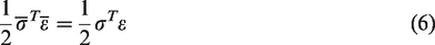
Alternatively, one can use the second hypothesis of equivalence. This is the hypothesis of elastic energy equivalence. In this hypothesis, the elastic energy is assumed to be equal in both configurations. This is expressed mathematically as follows:

\frac{1}{2} {\bar{σ}}^{T} \bar{ε} = \frac{1}{2} σ^{T} ε

(6)

One next substitutes the relations in equations (1) to (3) into equation (6) to obtain the following general transformation relation for the elasticity tensor:

E = [M^{- 1} + (I - M^{- 1}) : H^{- 1}] : \bar{E} : {[M^{- 1} + (I - M^{- 1}) : H^{- 1}]}^{T}

(7)

It should be noted that the general transformation equation for the elasticity tensor shown above is limited to the hypothesis of elastic energy equivalence. This transformation relation includes the effects of damage and healing through the use of the fourth-rank damage effect tensor and the fourth-rank healing tensor. Furthermore, it is noted that the general transformation equation for the elasticity tensor of equation (7) is far more complicated than that of equation (5). This is because the hypothesis of elastic energy equivalence is more sophisticated and physical based than the simple hypothesis of strain equivalence.

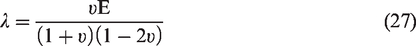
In equations (6) and (7), the superscript T indeed indicates the transpose of a tensor. For fourth-rank tensors, this can be most easily obtained from the 6 × 6 matrix representation of the tensor. The transpose of a matrix is obtained by switching or flipping all the off-diagonal terms like it is customary to do in matrix algebra. Then, the problem of the transpose of a fourth-rank tensor is reduced to the problem of the transpose of a matrix.

The expression of the fourth-rank constant elasticity tensor $\bar{E}$ is written as follows:

\bar{E} = λ I^{(2)} \otimes I^{(2)} + 2 μ I^{(2)} \bar{\otimes} I^{(2)}

(8)

where

λ

and

μ

are Lame’s constants and

I^{(2)}

is the second-rank identity tensor. Thus, the following expression for the variable fourth-rank elasticity tensor

E

(by adding fabric tensors) is obtained:

E = λ (G^{(0)} I^{(2)} + G^{(2)}) \otimes (G^{(0)} I^{(2)} + G^{(2)}) + 2 μ (G^{(0)} I^{(2)} + G^{(2)}) \bar{\otimes} (G^{(0)} I^{(2)} + G^{(2)})

(9)

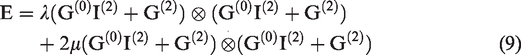
For more details on the definition of these two fabric tensors appearing in the equation above, the reader is referred to the work of Zysset and Curnier (1995) – see also Appendix 2.

Next, we consider the spectral decomposition of the second-rank fabric tensor $G^{(2)}$ as follows:

G^{(2)} = \sum_{i = 1}^{3} g_{i} (g_{i} \otimes g_{i})

(10)

where

g_{i} (i = 1, 2, 3)

are the eigenvalues of

G^{(2)}

and

g_{i} (i = 1, 2, 3)

are the corresponding eigenvectors. Zysset and Curnier (1995) used the terminology

G_{i}

to denote the cross product

g_{i} \otimes g_{i}

as follows:

G_{i} = g_{i} \otimes g_{i} (no sum over i)

(11)

where it is clear that

\sum_{i = 1}^{3} G_{i} = I^{(2)}

. Using this new terminology, one can write the following alternative expression for

E

which was derived in detail by Zysset and Curnier (1995):

E = (λ + 2 μ) m_{i}^{2 k} (G_{i} \otimes G_{i}) + λ m_{i}^{k} m_{j}^{k} (G_{i} \otimes G_{j} + G_{j} \otimes G_{i}) + 2 μ m_{i}^{k} m_{j}^{k} (G_{i} \otimes_{}^{-} G_{j} + G_{j} \otimes_{}^{-} G_{i})

(12)

where

k

is a constant scalar parameter and

m_{i}

is given by the following:

m_{i} = G^{(0)} + g_{i}

(13)

In the above equation, one notes that $\sum_{i = 1}^{3} m_{i} = constant$ . For the special case of isotropy, $g_{i} = 0, (i = 1, 2, 3)$ and $m_{i} = G^{(0)}, (i = 1, 2, 3)$ , so equation (12) reduces to the following equation of isotropic elasticity:

\begin{array}{l} E = (λ + 2 μ) g^{2 k} (G_{i} \otimes G_{i}) + λ g^{2 k} (G_{i} \otimes G_{j} + G_{j} \otimes G_{i}) + 2 μ g^{2 k} (G_{i} \otimes G_{j} + G_{j} \otimes G_{i}) \end{array}

(14)

The damage tensor, the healing tensor, and fabric tensors

In this section, an implicit expression for the damage and healing tensors in terms of the fabric tensors is derived. The expression to be derived will provide a link between damage mechanics, healing mechanics, and fabric tensors. It will provide the theory of damage and healing mechanics with a solid physical basis that directly depends on the micro-structure. It should be noted that no explicit expressions are possible, i.e. one will not be able to derive a direct explicit relation between the damage and healing tensors on the one hand, and fabric tensors on the other hand. The derived relationship is clearly implicit.

First, the hypothesis of strain equivalence is considered. Substituting for E from equation (5) into equation (9), one obtains the following relationship:

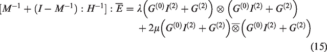
\begin{array}{l} [M^{- 1} + (I - M^{- 1}) : H^{- 1}] : \bar{E} = λ (G^{(0)} I^{(2)} + G^{(2)}) \otimes (G^{(0)} I^{(2)} + G^{(2)}) \\ + 2 μ (G^{(0)} I^{(2)} + G^{(2)}) \bar{\otimes} (G^{(0)} I^{(2)} + G^{(2)}) \end{array}

(15)

The above expression comprises an implicit relationship between the damage tensor M, the healing tensor H, and fabric tensors G⁽⁰⁾ and G⁽²⁾. In this relationship, the appearance of the effective elasticity tensor is noted. In the next few sections, this relationship of equation (15) will be used in several examples.

Next, one considers the hypothesis of elastic energy equivalence, In this case, one substitutes for the elasticity tensor E from equation (7) into equation (9) to obtain the following relationship:

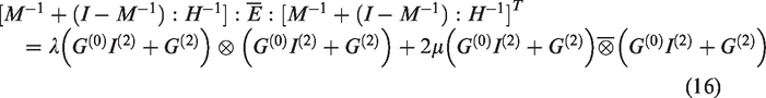
\begin{array}{l} [M^{- 1} + (I - M^{- 1}) : H^{- 1}] : \bar{E} : {[M^{- 1} + (I - M^{- 1}) : H^{- 1}]}^{T} \\ = λ (G^{(0)} I^{(2)} + G^{(2)}) \otimes (G^{(0)} I^{(2)} + G^{(2)}) + 2 μ (G^{(0)} I^{(2)} + G^{(2)}) \bar{\otimes} (G^{(0)} I^{(2)} + G^{(2)}) \end{array}

(16)

Equation (16) above represents an implicit relationship between the damage tensor M, the healing tensor H, and fabric tensors G⁽⁰⁾ and G⁽²⁾. It is noted that the effective elasticity tensor appears prominently in this relationship. Note that this relationship (equation (16)) for the hypothesis of elastic energy equivalence is far more complex than that obtained before (equation (15)) for the hypothesis of strain equivalence. In the next sections, this relationship of equation (16) will be used in several examples.

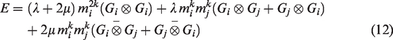
To conclude this section, one represents the elasticity tensor E of equations (12) and (14) in matrix form as follows where the parameters of the fabric tensors are clearly evident:

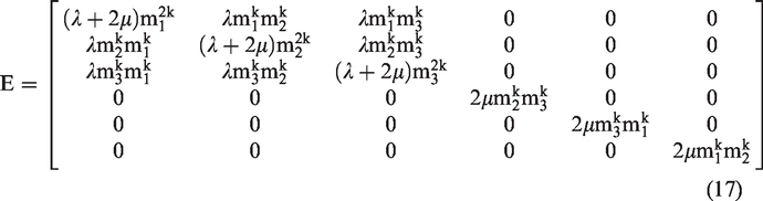
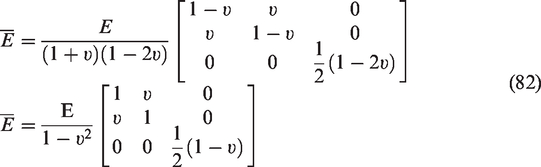
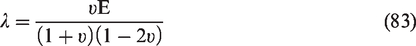
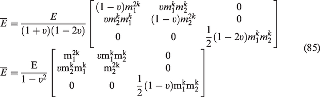
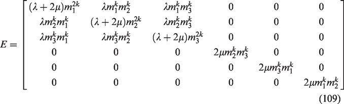
E = [\begin{matrix} (λ + 2 μ) m_{1}^{2 k} & λ m_{1}^{k} m_{2}^{k} & λ m_{1}^{k} m_{3}^{k} & 0 & 0 & 0 \\ λ m_{2}^{k} m_{1}^{k} & (λ + 2 μ) m_{2}^{2 k} & λ m_{2}^{k} m_{3}^{k} & 0 & 0 & 0 \\ λ m_{3}^{k} m_{1}^{k} & λ m_{3}^{k} m_{2}^{k} & (λ + 2 μ) m_{3}^{2 k} & 0 & 0 & 0 \\ 0 & 0 & 0 & 2 μ m_{2}^{k} m_{3}^{k} & 0 & 0 \\ 0 & 0 & 0 & 0 & 2 μ m_{3}^{k} m_{1}^{k} & 0 \\ 0 & 0 & 0 & 0 & 0 & 2 μ m_{1}^{k} m_{2}^{k} \end{matrix}]

(17)

In equation (17), the elasticity tensor E is represented in matrix form in terms of Lame’s constants λ and μ, and the various parameters of the fabric tensors m₁, m₂, and k. This matrix representation will be used in some of the examples below. It should be noted that equation (17) applies to isotropic materials and it is used extensively later in Section ‘Example III – Isotropic elasticity, isotropic damage, and isotropic healing’ on isotropic elasticity.

Example I – plane stress, plane damage, and plane healing

Next, the example of plane stress in the $x_{1} - x_{2}$ plane is shown. The following notation of vectors will be used:

σ = {[\begin{matrix} σ_{11} & σ_{22} & σ_{12} \end{matrix}]}^{T}

(18)

ε = {[\begin{matrix} ε_{11} & ε_{22} & ε_{12} \end{matrix}]}^{T}

(19)

Similarly, the effective stress tensor can be represented by the following 3 × 1 vector:

\bar{σ} = {[\begin{matrix} {\bar{σ}}_{11} & {\bar{σ}}_{22} & {\bar{σ}}_{12} \end{matrix}]}^{T}

(20)

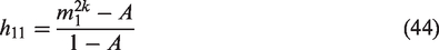
Next, the fourth-rank damage effect tensor M can be represented by the following 3 × 3 matrix for the case of plane stress. In this equation, one assumes a state of plane damage in addition to the state of plane stress.

M = \frac{1}{Δ} [\begin{matrix} ψ_{22} & 0 & φ_{12} \\ 0 & ψ_{11} & φ_{12} \\ \frac{1}{2} φ_{12} & \frac{1}{2} φ_{12} & \frac{1}{2} (ψ_{11} + ψ_{22}) \end{matrix}]

(21)

where

Δ = ψ_{11} ψ_{22} - φ_{12}^{2}

(22)

ψ_{11} = 1 - φ_{11}

(23)

ψ_{22} = 1 - φ_{22}

(24)

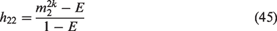
In addition, the fourth-rank healing tensor H can be represented by the following 3 × 3 matrix for the case of plane stress. In this equation, one assumes a state of plane healing in addition to the states of plane stress and plane damage.

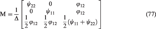
H^{- 1} = [\begin{matrix} h_{11} & 0 & h_{12} \\ 0 & h_{22} & h_{12} \\ h_{12} & h_{12} & \frac{1}{2} (h_{11} + h_{22}) \end{matrix}]

(25)

The effective elasticity tensor for this case is given by the following 3 × 3 matrix:

\bar{E} = \frac{E}{1 - υ^{2}} [\begin{matrix} 1 & υ & 0 \\ υ & 1 & 0 \\ 0 & 0 & \frac{1}{2} (1 - υ) \end{matrix}]

(26)

where,

λ = \frac{υ E}{(1 + υ) (1 - 2 υ)}

(27)

μ = \frac{E}{2 (1 + υ)}

(28)

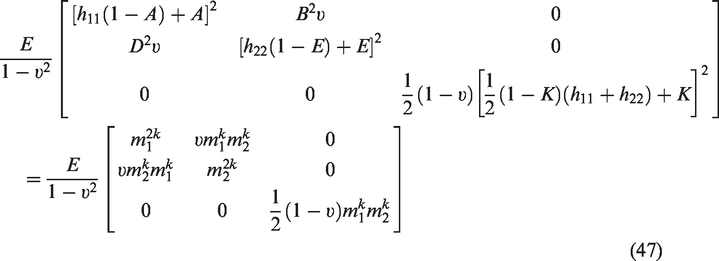
Finally, the elasticity tensor E in the damaged and healed configuration is represented as follows in terms of fabric tensor parameters (based on equation (17)):

\bar{E} = \frac{E}{1 - υ^{2}} [\begin{matrix} m_{1}^{2 k} & υ m_{1}^{k} m_{2}^{k} & 0 \\ υ m_{2}^{k} m_{1}^{k} & m_{2}^{2 k} & 0 \\ 0 & 0 & \frac{1}{2} (1 - υ) m_{1}^{k} m_{2}^{k} \end{matrix}]

(29)

Next, one derives the respective general equations for fabric tensors with damage and healing for the case of plane stress for both the hypothesis of strain equivalence and the hypothesis of elastic energy equivalence.

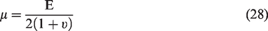
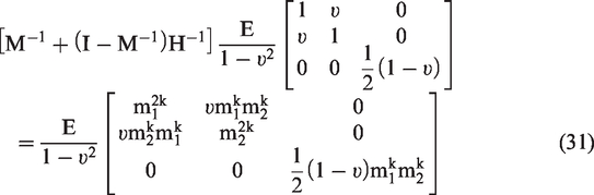
First, one considers the hypothesis of strain equivalence. Substituting the respective 3 × 3 matrices of plane stress from equations (21), (25), (26), and (29) into equation (5), one obtains:

\begin{array}{l} {\begin{cases} Δ {[\begin{matrix} ψ_{22} & 0 & φ_{12} \\ 0 & ψ_{11} & φ_{12} \\ \frac{1}{2} φ_{12} & \frac{1}{2} φ_{12} & \frac{1}{2} (ψ_{11} + ψ_{22}) \end{matrix}]}^{- 1} + ([\begin{matrix} 1 & 0 & 0 \\ 0 & 1 & 0 \\ 0 & 0 & 1 \end{matrix}] - Δ {[\begin{matrix} ψ_{22} & 0 & φ_{12} \\ 0 & ψ_{11} & φ_{12} \\ \frac{1}{2} φ_{12} & \frac{1}{2} φ_{12} & \frac{1}{2} (ψ_{11} + ψ_{22}) \end{matrix}]}^{- 1}) \\ * [\begin{matrix} h_{11} & 0 & h_{12} \\ 0 & h_{22} & h_{12} \\ h_{12} & h_{12} & \frac{1}{2} (h_{11} + h_{22}) \end{matrix}] \end{cases}} \\ * \frac{E}{1 - υ^{2}} [\begin{matrix} 1 & υ & 0 \\ υ & 1 & 0 \\ 0 & 0 & \frac{1}{2} (1 - υ) \end{matrix}] = \frac{E}{1 - υ^{2}} [\begin{matrix} m_{1}^{2 k} & υ m_{1}^{k} m_{2}^{k} & 0 \\ υ m_{2}^{k} m_{1}^{k} & m_{2}^{2 k} & 0 \\ 0 & 0 & \frac{1}{2} (1 - υ) m_{1}^{k} m_{2}^{k} \end{matrix}] \end{array}

(30)

One next contracts the above equation and re-writes it as follows:

[M^{- 1} + (I - M^{- 1}) H^{- 1}] \frac{E}{1 - υ^{2}} [\begin{matrix} 1 & υ & 0 \\ υ & 1 & 0 \\ 0 & 0 & \frac{1}{2} (1 - υ) \end{matrix}] = \frac{E}{1 - υ^{2}} [\begin{matrix} m_{1}^{2 k} & υ m_{1}^{k} m_{2}^{k} & 0 \\ υ m_{2}^{k} m_{1}^{k} & m_{2}^{2 k} & 0 \\ 0 & 0 & \frac{1}{2} (1 - υ) m_{1}^{k} m_{2}^{k} \end{matrix}]

(31)

The inverse matrix of M will be shown shortly. Next, one considers the hypothesis of elastic energy equivalence. For this case, one substitutes the 3 × 3 matrix equations of plane stress (21), (25), (26), and (29) into equation (7) to obtain:

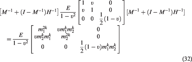
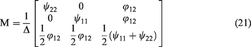
\begin{array}{l} [M^{- 1} + (I - M^{- 1}) H^{- 1}] \frac{E}{1 - υ^{2}} [\begin{matrix} 1 & υ & 0 \\ υ & 1 & 0 \\ 0 & 0 & \frac{1}{2} (1 - υ) \end{matrix}] [M^{- 1} + (I - M^{- 1}) H^{- 1}] \\ = \frac{E}{1 - υ^{2}} [\begin{matrix} m_{1}^{2 k} & υ m_{1}^{k} m_{2}^{k} & 0 \\ υ m_{2}^{k} m_{1}^{k} & m_{2}^{2 k} & 0 \\ 0 & 0 & \frac{1}{2} (1 - υ) m_{1}^{k} m_{2}^{k} \end{matrix}] \end{array}

(32)

In equations (31) and (32), one establishes the general equations of fabric tensors with damage and healing for the hypothesis of strain equivalence and the hypothesis of elastic energy equivalence, respectively.

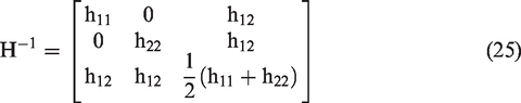
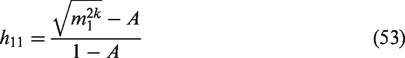
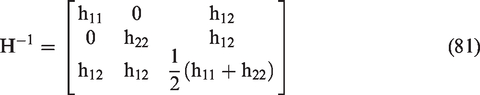
In equations (31) and (32), one notices the presence of the inverse of M. This inverse matrix is obtained using Mathematica as follows:

M^{- 1} = \frac{Δ}{Ω} [\begin{matrix} ψ_{22} ψ_{11} + φ_{12}^{2} + ψ_{11}^{2} - 2 ψ_{11} & - φ_{12}^{2} & 2 φ_{12} ψ_{11} \\ - φ_{12}^{2} & ψ_{22}^{2} + ψ_{22} ψ_{11} - 2 ψ_{22} + φ_{12}^{2} & 2 φ_{12} ψ_{22} \\ φ_{12} ψ_{11} & φ_{12} ψ_{22} & - 2 ψ_{22} ψ_{11} \end{matrix}]

(33)

where

Δ = ψ_{11} ψ_{22} - φ_{12}^{2}

(34)

Ω = ψ_{22}^{2} ψ_{11} + ψ_{22} [φ_{12}^{2} + (ψ_{11} - 2) ψ_{11}] + φ_{12}^{2} ψ_{11}

(35)

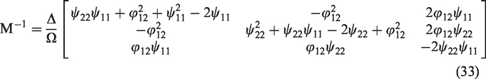
Equation (33) can be re-written in the following more suitable form:

M^{- 1} = [\begin{matrix} A & B & C \\ D & E & F \\ G & H & K \end{matrix}]

(36)

where the various symbols in the matrix of equation (36) can be readily obtained from the expressions in equation (33). These symbols are explicitly presented in Appendix 1.

For the hypothesis of strain equivalence and using the inverse matrix of equation (36) and substituting it into equation (31), the latter equation becomes after tremendous simplifications performed using Mathematica:

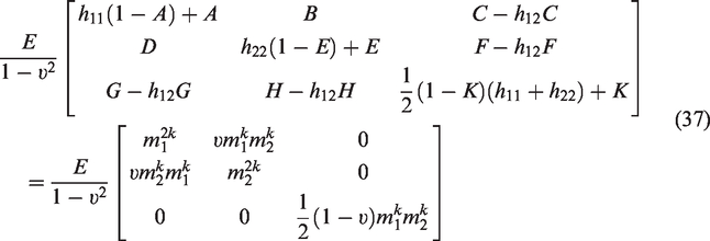
\begin{array}{l} \frac{E}{1 - υ^{2}} [\begin{matrix} h_{11} (1 - A) + A & B & C - h_{12} C \\ D & h_{22} (1 - E) + E & F - h_{12} F \\ G - h_{12} G & H - h_{12} H & \frac{1}{2} (1 - K) (h_{11} + h_{22}) + K \end{matrix}] \\ = \frac{E}{1 - υ^{2}} [\begin{matrix} m_{1}^{2 k} & υ m_{1}^{k} m_{2}^{k} & 0 \\ υ m_{2}^{k} m_{1}^{k} & m_{2}^{2 k} & 0 \\ 0 & 0 & \frac{1}{2} (1 - υ) m_{1}^{k} m_{2}^{k} \end{matrix}] \end{array}

(37)

The above matrix equation can be re-written as the following set of five simultaneous algebraic scalar equations:

h_{11} (1 - A) + A = m_{1}^{2 k}

(38)

B υ = υ m_{1}^{k} m_{2}^{k}

(39)

D υ = υ m_{2}^{k} m_{1}^{k}

(40)

h_{22} (1 - E) + E = m_{2}^{2 k}

(41)

\frac{1}{2} (1 - υ) [\frac{1}{2} (1 - K) (h_{11} + h_{22}) + K] = \frac{1}{2} (1 - υ) m_{1}^{k} m_{2}^{k}

(42)

The above set of equations can be simplified to be written in the following form:

B = D = m_{1}^{k} m_{2}^{k}

(43)

h_{11} = \frac{m_{1}^{2 k} - A}{1 - A}

(44)

h_{22} = \frac{m_{2}^{2 k} - E}{1 - E}

(45)

\frac{1}{2} (1 - K) (\frac{m_{1}^{2 k} - A}{1 - A} + \frac{m_{2}^{2 k} - E}{1 - E}) + K = m_{1}^{k} m_{2}^{k}

(46)

The above set of equation comprise the governing equations for plane stress for the hypothesis of strain equivalence.

Similar to equation (37), the following general equation can be obtained for the hypothesis of elastic energy equivalence:

\begin{array}{l} \frac{E}{1 - υ^{2}} [\begin{matrix} {[h_{11} (1 - A) + A]}^{2} & B^{2} υ & 0 \\ D^{2} υ & {[h_{22} (1 - E) + E]}^{2} & 0 \\ 0 & 0 & \frac{1}{2} (1 - υ) {[\frac{1}{2} (1 - K) (h_{11} + h_{22}) + K]}^{2} \end{matrix}] \\ = \frac{E}{1 - υ^{2}} [\begin{matrix} m_{1}^{2 k} & υ m_{1}^{k} m_{2}^{k} & 0 \\ υ m_{2}^{k} m_{1}^{k} & m_{2}^{2 k} & 0 \\ 0 & 0 & \frac{1}{2} (1 - υ) m_{1}^{k} m_{2}^{k} \end{matrix}] \end{array}

(47)

The above matrix equation can be re-written as the following set of five simultaneous algebraic scalar equations:

{[h_{11} (1 - A) + A]}^{2} = m_{1}^{2 k}

(48)

B^{2} υ = υ m_{1}^{k} m_{2}^{k}

(49)

D^{2} υ = υ m_{2}^{k} m_{1}^{k}

(50)

{[h_{22} (1 - E) + E]}^{2} = m_{2}^{2 k}

(51)

\frac{1}{2} (1 - υ) {[\frac{1}{2} (1 - K) (h_{11} + h_{22}) + K]}^{2} = \frac{1}{2} (1 - υ) m_{1}^{k} m_{2}^{k}

(52)

The above set of equations can be simplified to be written as follows:

h_{11} = \frac{\sqrt{m_{1}^{2 k}} - A}{1 - A}

(53)

B^{2} = D^{2} = m_{1}^{k} m_{2}^{k}

(54)

h_{22} = \frac{\sqrt{m_{2}^{2 k}} - E}{1 - E}

(55)

{[\frac{1}{2} (1 - K) (\frac{\sqrt{m_{1}^{2 k}} - A}{1 - A} + \frac{\sqrt{m_{2}^{2 k}} - E}{1 - E}) + K]}^{2} = m_{1}^{k} m_{2}^{k}

(56)

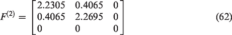
The above set of equations comprise the governing equations for plane stress for the hypothesis of elastic energy equivalence.

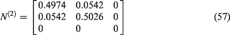
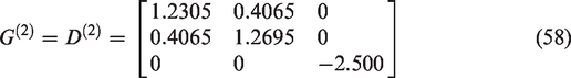
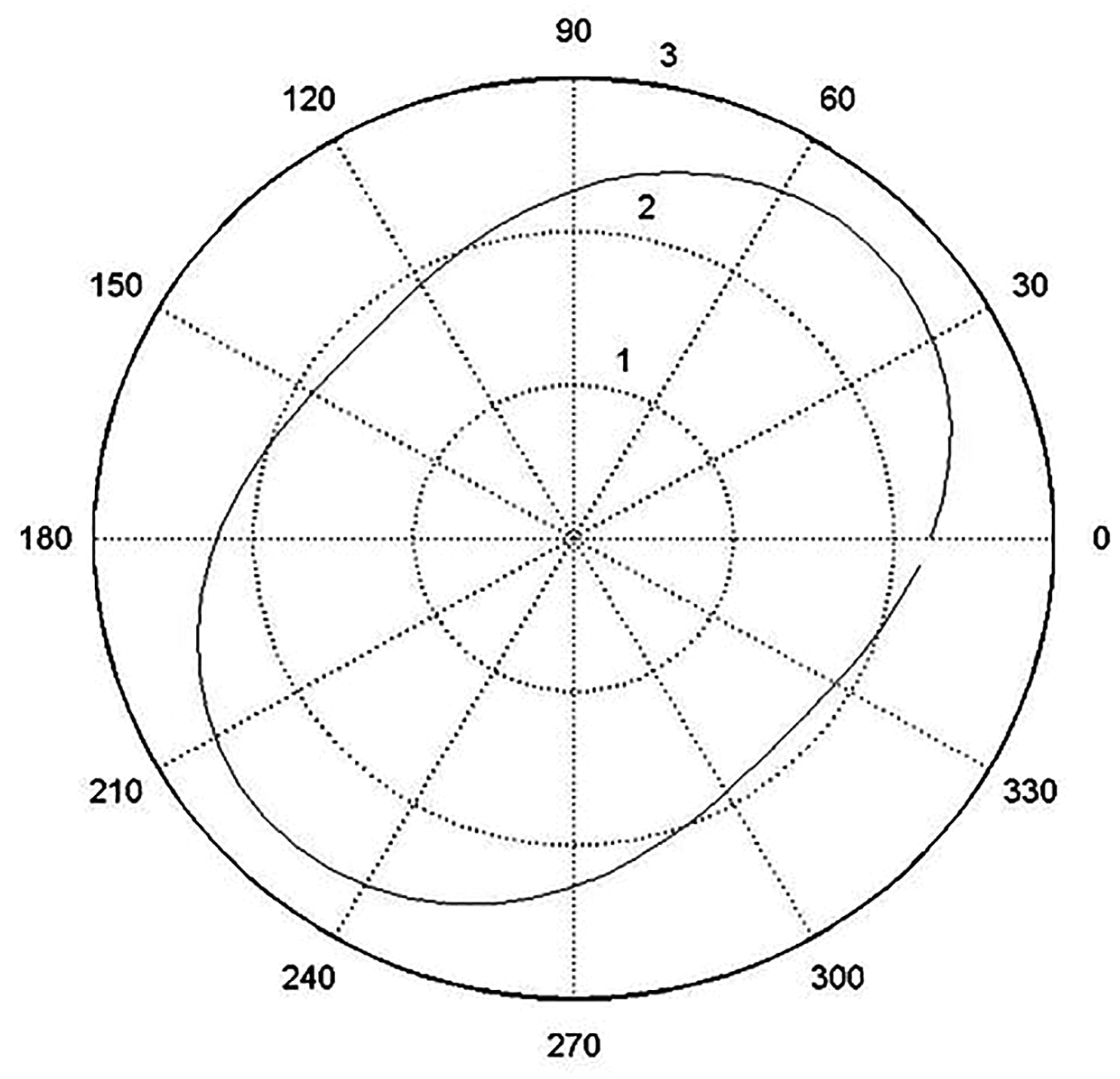
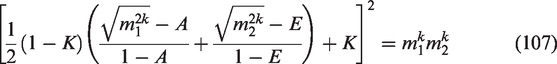
Next, a numerical example is solved for a particular micro-crack distribution based on the plane stress case. The micro-crack distribution is presented in the form of a circular histogram (rose diagram) as shown in Figure 3. The various fabric tensors are calculated for this micro-crack distribution using the formulas listed in Appendix 2. The resulting matrices are listed below. The numbers in equations (57) to (63) are determined using the formulas of fabric tensors listed in Appendix 2 along with using the data from the circular histogram of Figure 3:

N^{(2)} = [\begin{array}{l} 0.4974 & 0.0542 & 0 \\ 0.0542 & 0.5026 & 0 \\ 0 & 0 & 0 \end{array}]

(57)

G^{(2)} = D^{(2)} = [\begin{array}{l} 1.2305 & 0.4065 & 0 \\ 0.4065 & 1.2695 & 0 \\ 0 & 0 & - 2.500 \end{array}]

(58)

g_{1} = 1.6570

(59)

g_{2} = 0.8430

(60)

g_{3} = - 2.500

(61)

F^{(2)} = [\begin{array}{l} 2.2305 & 0.4065 & 0 \\ 0.4065 & 2.2695 & 0 \\ 0 & 0 & 0 \end{array}]

(62)

ρ (n) = 2.2305 \cos^{2} θ + 2.2695 \sin^{2} θ + 0.8130 \sin θ \cos θ

(63)

Figure 3.

The micro-crack distribution represented by a rose diagram or also called a circular histogram.

The second-order approximation of equation (63) is presented in the form of a polar plot as shown in Figure 4.

Figure 4.

This is a second-order approximation of the micro-crack distribution in the form of a polar plot.

Finally, the following numerical values are used in this example:

m_{1} + m_{2} = 2 G^{(0)} + g_{1} + g_{2}

(64)

G^{(0)} = 1

(65)

m_{1} + m_{2} = 4.5

(66)

υ = 0.3

(67)

k = - 0.2

(68)

m_{2} = 4.5 - m_{1}

(69)

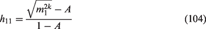
From equation (38) for the hypothesis of strain equivalence, and using the numerical values above, one concludes the following final relation:

m_{1} = \frac{1}{{\sqrt{[1 - φ_{11} (1 - h_{11})]}}^{5}}

(70)

m_{2} = \frac{1}{{\sqrt{[1 - φ_{22} (1 - h_{22})]}}^{5}}

(71)

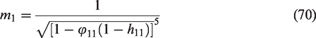
The relation in equation (70) is plotted with a three-dimensional graph and is shown in Figure 5. This figure applies to the case of plane stress for the hypothesis of strain equivalence for the specified micro-crack distribution. From this figure it is seen that the fabric tensor parameter m₁ reaches values up to 8 and climaxes into a plateau at the extreme end of the damage tensor values. A similar graph is obtained for m₂ of equation (71) but is not shown here.

Figure 5.

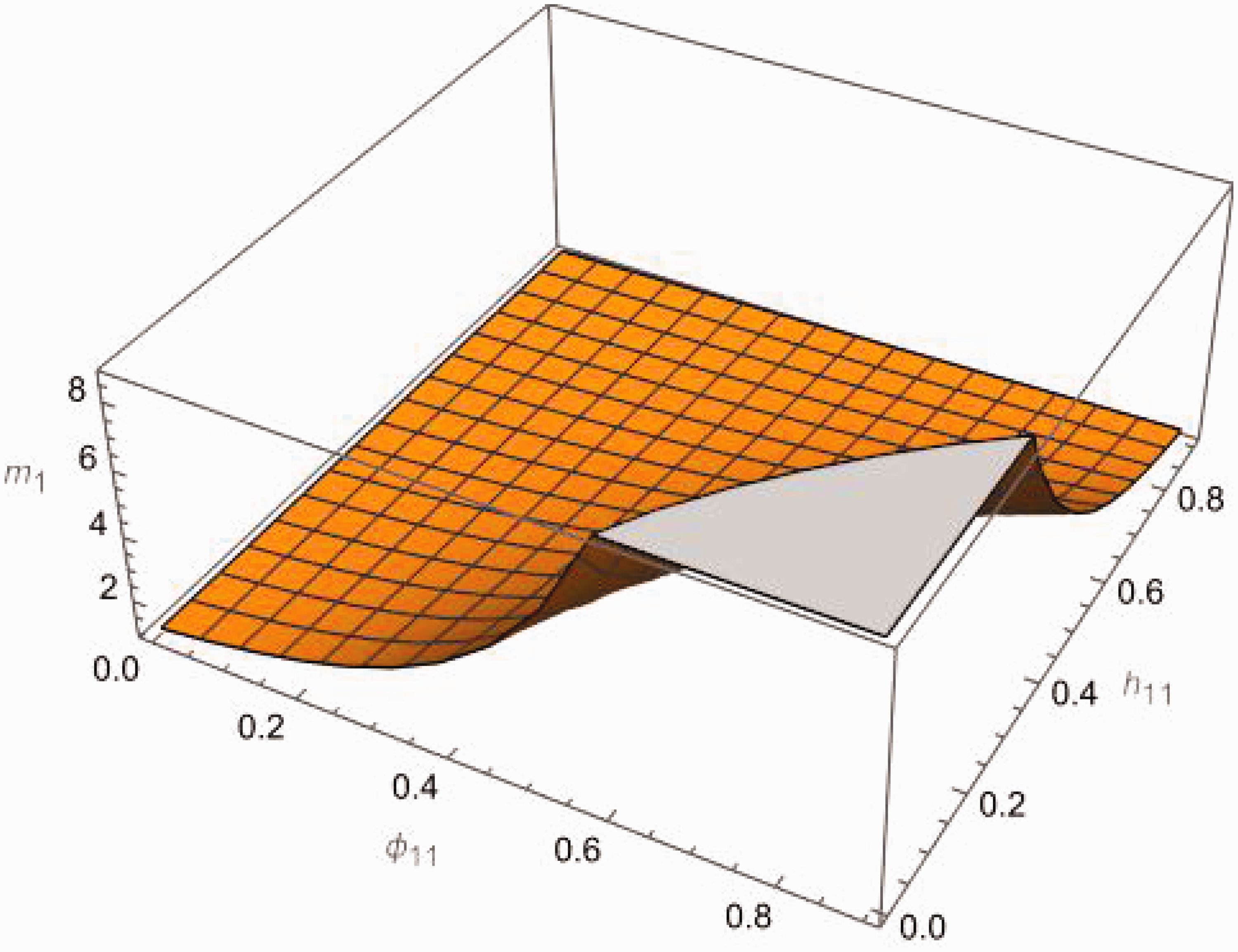
Hypothesis of strain equivalence showing the relationship between the various tensor components.

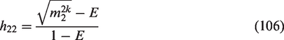
From equation (48) for the hypothesis of elastic energy equivalence, and using the numerical values above, one concludes the following final relation:

m_{1} = \frac{1}{{[1 - φ_{11} (1 - h_{11})]}^{5}}

(72)

m_{2} = \frac{1}{{[1 - φ_{22} (1 - h_{22})]}^{5}}

(73)

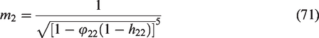
The relation in equation (72) is plotted with a three-dimensional graph and is shown in Figure 6. This figure applies to the case of plane stress for the hypothesis of elastic energy equivalence for the specified micro-crack distribution. From this figure it is seen that the fabric tensor parameter m₁ reaches values up to 40 and climaxes into a plateau at the extreme end of the damage tensor values. A similar graph is obtained for m₂ of equation (73) but is not shown here. It is noted that significantly higher values of the fabric tensor parameters are obtained for the hypothesis of elastic energy equivalence compared with the hypothesis of strain equivalence. This is clearly seen by comparing Figures 5 and 6.

Figure 6.

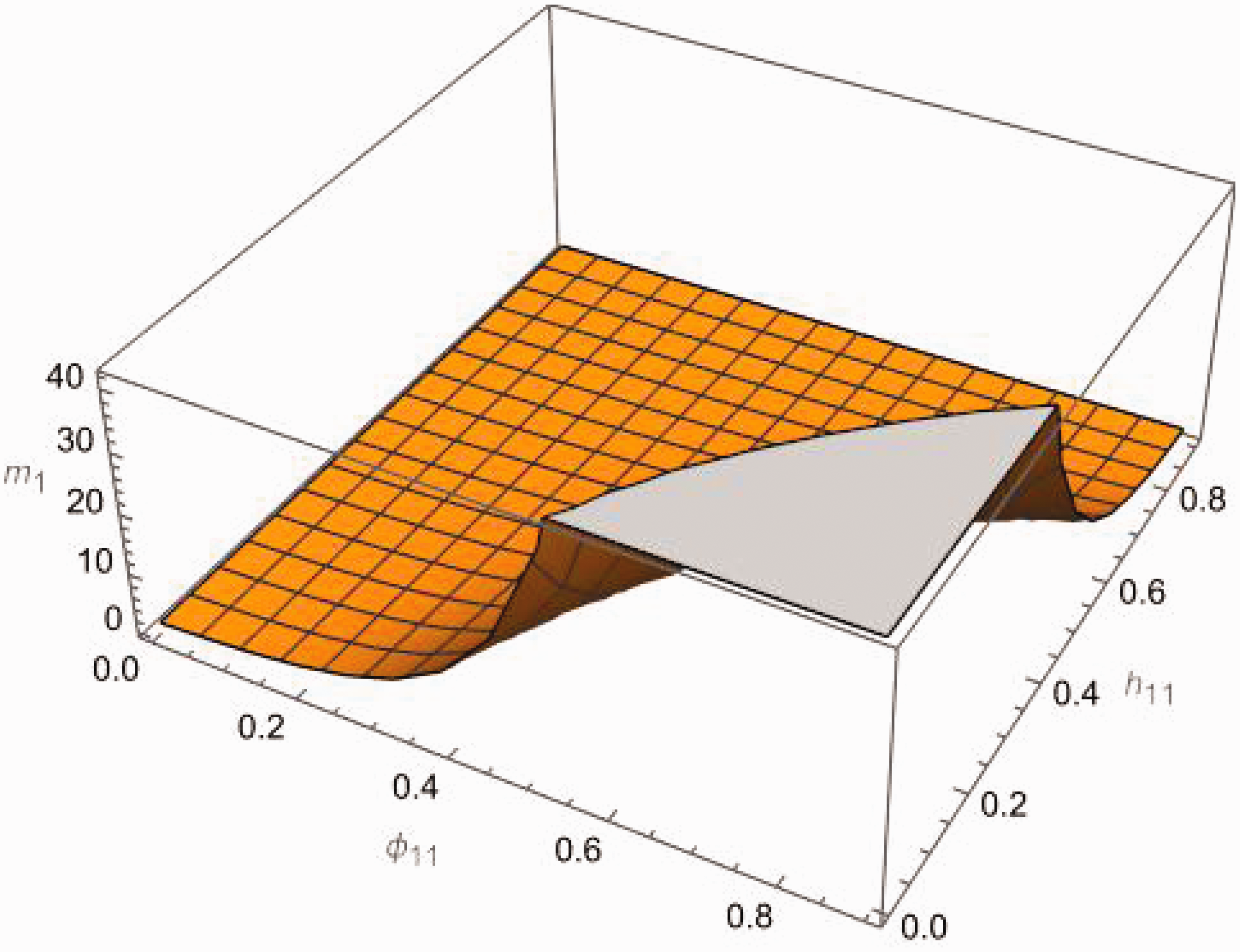
Hypothesis of elastic energy equivalence showing the relationship between the various tensor components.

Example II – plane strain, plane damage, and plane healing

One next considers the case of plane strain in the $x_{1} - x_{2}$ plane. The equations of fabric tensors with damage and healing for this case are derived. In this case the stress and strain tensors can be represented by the following 3 × 1 vectors:

σ = {[\begin{matrix} σ_{11} & σ_{22} & σ_{12} \end{matrix}]}^{T}

(74)

ε = {[\begin{matrix} ε_{11} & ε_{22} & ε_{12} \end{matrix}]}^{T}

(75)

Similarly, the effective stress tensor can be represented by the following 3 × 1 vector:

\bar{σ} = {[\begin{matrix} {\bar{σ}}_{11} & {\bar{σ}}_{22} & {\bar{σ}}_{12} \end{matrix}]}^{T}

(76)

Next, the fourth-rank damage effect tensor M can be represented by the following 3 × 3 matrix for the case of plane strain. In this equation, one assumes a state of plane damage in addition to the state of plane stress.

M = \frac{1}{Δ} [\begin{matrix} ψ_{22} & 0 & φ_{12} \\ 0 & ψ_{11} & φ_{12} \\ \frac{1}{2} φ_{12} & \frac{1}{2} φ_{12} & \frac{1}{2} (ψ_{11} + ψ_{22}) \end{matrix}]

(77)

where

Δ = ψ_{11} ψ_{22} - φ_{12}^{2}

(78)

ψ_{11} = 1 - φ_{11}

(79)

ψ_{22} = 1 - φ_{22}

(80)

In addition, the fourth-rank healing tensor H can be represented by the following 3 × 3 matrix for the case of plane strain. In this equation, one assumes a state of plane healing in addition to the states of plane strain and plane damage.

H^{- 1} = [\begin{matrix} h_{11} & 0 & h_{12} \\ 0 & h_{22} & h_{12} \\ h_{12} & h_{12} & \frac{1}{2} (h_{11} + h_{22}) \end{matrix}]

(81)

The effective elasticity tensor for this case is given by the following 3 × 3 matrix:

\begin{array}{l} \bar{E} = \frac{E}{(1 + υ) (1 - 2 υ)} [\begin{matrix} 1 - υ & υ & 0 \\ υ & 1 - υ & 0 \\ 0 & 0 & \frac{1}{2} (1 - 2 υ) \end{matrix}] \\ \bar{E} = \frac{E}{1 - υ^{2}} [\begin{matrix} 1 & υ & 0 \\ υ & 1 & 0 \\ 0 & 0 & \frac{1}{2} (1 - υ) \end{matrix}] \end{array}

(82)

where

λ = \frac{υ E}{(1 + υ) (1 - 2 υ)}

(83)

μ = \frac{E}{2 (1 + υ)}

(84)

Finally, the elasticity tensor E in the damaged and healed configuration is represented as follows in terms of fabric tensor parameters (based on equation (17)):

\begin{array}{l} \bar{E} = \frac{E}{(1 + υ) (1 - 2 υ)} [\begin{matrix} (1 - υ) m_{1}^{2 k} & υ m_{1}^{k} m_{2}^{k} & 0 \\ υ m_{2}^{k} m_{1}^{k} & (1 - υ) m_{2}^{2 k} & 0 \\ 0 & 0 & \frac{1}{2} (1 - 2 υ) m_{1}^{k} m_{2}^{k} \end{matrix}] \\ \bar{E} = \frac{E}{1 - υ^{2}} [\begin{matrix} m_{1}^{2 k} & {υm}_{1}^{k} m_{2}^{k} & 0 \\ {υm}_{2}^{k} m_{1}^{k} & m_{2}^{2 k} & 0 \\ 0 & 0 & \frac{1}{2} (1 - υ) m_{1}^{k} m_{2}^{k} \end{matrix}] \end{array}

(85)

Next, one derives the respective general equations for fabric tensors with damage and healing for the case of plane strain for both the hypothesis of strain equivalence and the hypothesis of elastic energy equivalence.

First, one considers the hypothesis of strain equivalence. Substituting the respective 3 × 3 matrices of plane strain from equations (77), (81), (82), and (85) into equation (5), one obtains:

\begin{array}{l} {\begin{cases} Δ {[\begin{matrix} ψ_{22} & 0 & φ_{12} \\ 0 & ψ_{11} & φ_{12} \\ \frac{1}{2} φ_{12} & \frac{1}{2} φ_{12} & \frac{1}{2} (ψ_{11} + ψ_{22}) \end{matrix}]}^{- 1} + ([\begin{matrix} 1 & 0 & 0 \\ 0 & 1 & 0 \\ 0 & 0 & 1 \end{matrix}] - Δ {[\begin{matrix} ψ_{22} & 0 & φ_{12} \\ 0 & ψ_{11} & φ_{12} \\ \frac{1}{2} φ_{12} & \frac{1}{2} φ_{12} & \frac{1}{2} (ψ_{11} + ψ_{22}) \end{matrix}]}^{- 1}) \\ * [\begin{matrix} h_{11} & 0 & h_{12} \\ 0 & h_{22} & h_{12} \\ h_{12} & h_{12} & \frac{1}{2} (h_{11} + h_{22}) \end{matrix}] \end{cases}} \\ * \frac{E}{(1 + υ) (1 - 2 υ)} [\begin{matrix} 1 - υ & υ & 0 \\ υ & 1 - υ & 0 \\ 0 & 0 & \frac{1}{2} (1 - 2 υ) \end{matrix}] \\ = \frac{E}{(1 + υ) (1 - 2 υ)} [\begin{matrix} (1 - υ) m_{1}^{2 k} & υ m_{1}^{k} m_{2}^{k} & 0 \\ υ m_{2}^{k} m_{1}^{k} & (1 - υ) m_{2}^{2 k} & 0 \\ 0 & 0 & \frac{1}{2} (1 - 2 υ) m_{1}^{k} m_{2}^{k} \end{matrix}] \\ = \frac{E}{1 - υ^{2}} [\begin{matrix} m_{1}^{2 k} & {υm}_{1}^{k} m_{2}^{k} & 0 \\ {υm}_{2}^{k} m_{1}^{k} & m_{2}^{2 k} & 0 \\ 0 & 0 & \frac{1}{2} (1 - υ) m_{1}^{k} m_{2}^{k} \end{matrix}] \end{array}

(86)

One next contracts the above equation and re-writes it as follows:

\begin{array}{l} \frac{E}{(1 + υ) (1 - 2 υ)} [\begin{matrix} (1 - υ) [h_{11} (1 - A) + A] & B υ & 0 \\ D υ & (1 - υ) [h_{22} (1 - E) + E] & 0 \\ 0 & 0 & \frac{1}{2} (1 - 2 υ) [(1 - K) (h_{11} + h_{22}) + K] \end{matrix}] \\ = \frac{E}{(1 + υ) (1 - 2 υ)} [\begin{matrix} (1 - υ) m_{1}^{2 k} & υ m_{1}^{k} m_{2}^{k} & 0 \\ υ m_{2}^{k} m_{1}^{k} & (1 - υ) m_{2}^{2 k} & 0 \\ 0 & 0 & \frac{1}{2} (1 - 2 υ) m_{1}^{k} m_{2}^{k} \end{matrix}] \\ [M^{- 1} + (I - M^{- 1}) H^{- 1}] \frac{E}{1 - υ^{2}} [\begin{matrix} 1 & υ & 0 \\ υ & 1 & 0 \\ 0 & 0 & \frac{1}{2} (1 - υ) \end{matrix}] \\ = \frac{E}{1 - υ^{2}} [\begin{matrix} m_{1}^{2 k} & {υm}_{1}^{k} m_{2}^{k} & 0 \\ {υm}_{2}^{k} m_{1}^{k} & m_{2}^{2 k} & 0 \\ 0 & 0 & \frac{1}{2} (1 - υ) m_{1}^{k} m_{2}^{k} \end{matrix}] \end{array}

(87)

The inverse matrix of M was shown previously in Section ‘Example I – Plane stress, plane damage, and plane healing’ (see also Appendix 1). Next, one considers the hypothesis of elastic energy equivalence. For this case, we substitute the 3 × 3 matrix equations of plane strain (77), (81), (82), and (85) into equation (7) to obtain:

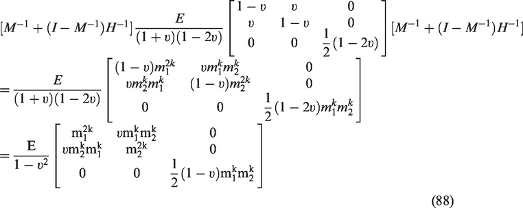
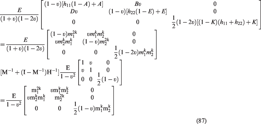
\begin{array}{l} [M^{- 1} + (I - M^{- 1}) H^{- 1}] \frac{E}{(1 + υ) (1 - 2 υ)} [\begin{matrix} 1 - υ & υ & 0 \\ υ & 1 - υ & 0 \\ 0 & 0 & \frac{1}{2} (1 - 2 υ) \end{matrix}] [M^{- 1} + (I - M^{- 1}) H^{- 1}] \\ = \frac{E}{(1 + υ) (1 - 2 υ)} [\begin{matrix} (1 - υ) m_{1}^{2 k} & υ m_{1}^{k} m_{2}^{k} & 0 \\ υ m_{2}^{k} m_{1}^{k} & (1 - υ) m_{2}^{2 k} & 0 \\ 0 & 0 & \frac{1}{2} (1 - 2 υ) m_{1}^{k} m_{2}^{k} \end{matrix}] \\ = \frac{E}{1 - υ^{2}} [\begin{matrix} m_{1}^{2 k} & {υm}_{1}^{k} m_{2}^{k} & 0 \\ {υm}_{2}^{k} m_{1}^{k} & m_{2}^{2 k} & 0 \\ 0 & 0 & \frac{1}{2} (1 - υ) m_{1}^{k} m_{2}^{k} \end{matrix}] \end{array}

(88)

In equations (87) and (88), one establishes the general equations of fabric tensors with damage and healing for the hypothesis of strain equivalence and the hypothesis of elastic energy equivalence, respectively.

Upon further substitutions, the equation (88) reduces to the following matrix relation:

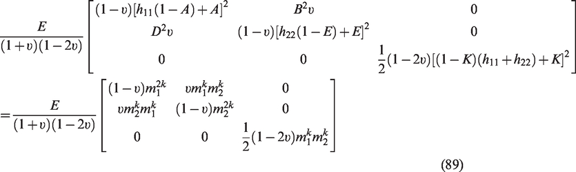
\begin{array}{l} \frac{E}{(1 + υ) (1 - 2 υ)} [\begin{matrix} (1 - υ) {[h_{11} (1 - A) + A]}^{2} & B^{2} υ & 0 \\ D^{2} υ & (1 - υ) {[h_{22} (1 - E) + E]}^{2} & 0 \\ 0 & 0 & \frac{1}{2} (1 - 2 υ) {[(1 - K) (h_{11} + h_{22}) + K]}^{2} \end{matrix}] \\ = \frac{E}{(1 + υ) (1 - 2 υ)} [\begin{matrix} (1 - υ) m_{1}^{2 k} & υ m_{1}^{k} m_{2}^{k} & 0 \\ υ m_{2}^{k} m_{1}^{k} & (1 - υ) m_{2}^{2 k} & 0 \\ 0 & 0 & \frac{1}{2} (1 - 2 υ) m_{1}^{k} m_{2}^{k} \end{matrix}] \end{array}

(89)

Equation (87) for the hypothesis of strain equivalence can be re-written as the following set of five simultaneous algebraic scalar equations:

(1 - υ) [h_{11} (1 - A) + A] = (1 - υ) m_{1}^{2 k}

(90)

B υ = υ m_{1}^{k} m_{2}^{k}

(91)

D υ = υ m_{2}^{k} m_{1}^{k}

(92)

(1 - υ) [h_{22} (1 - E) + E] = (1 - υ) m_{2}^{2 k}

(93)

\frac{1}{2} (1 - 2 υ) [\frac{1}{2} (1 - K) (h_{11} + h_{22}) + K] = \frac{1}{2} (1 - 2 υ) m_{1}^{k} m_{2}^{k}

(94)

The above set of equations can be simplified to be written in the following form:

B = D = m_{1}^{k} m_{2}^{k}

(95)

h_{11} = \frac{m_{1}^{2 k} - A}{1 - A}

(96)

h_{22} = \frac{m_{2}^{2 k} - E}{1 - E}

(97)

\frac{1}{2} (1 - K) (\frac{m_{1}^{2 k} - A}{1 - A} + \frac{m_{2}^{2 k} - E}{1 - E}) + K = m_{1}^{k} m_{2}^{k}

(98)

The above set of equation comprise the governing equations for plane strain for the hypothesis of strain equivalence.

Equation (89) for the hypothesis of elastic energy equivalence can be re-written as the following set of five simultaneous algebraic scalar equations:

(1 - υ) {[h_{11} (1 - A) + A]}^{2} = (1 - υ) m_{1}^{2 k}

(99)

B^{2} υ = υ m_{1}^{k} m_{2}^{k}

(100)

D^{2} υ = υ m_{2}^{k} m_{1}^{k}

(101)

(1 - υ) {[h_{22} (1 - E) + E]}^{2} = (1 - υ) m_{2}^{2 k}

(102)

\frac{1}{2} (1 - 2 υ) {[\frac{1}{2} (1 - K) (h_{11} + h_{22}) + K]}^{2} = \frac{1}{2} (1 - 2 υ) m_{1}^{k} m_{2}^{k}

(103)

The above set of equations can be simplified to be written as follows:

h_{11} = \frac{\sqrt{m_{1}^{2 k}} - A}{1 - A}

(104)

B^{2} = D^{2} = m_{1}^{k} m_{2}^{k}

(105)

h_{22} = \frac{\sqrt{m_{2}^{2 k}} - E}{1 - E}

(106)

{[\frac{1}{2} (1 - K) (\frac{\sqrt{m_{1}^{2 k}} - A}{1 - A} + \frac{\sqrt{m_{2}^{2 k}} - E}{1 - E}) + K]}^{2} = m_{1}^{k} m_{2}^{k}

(107)

The above set of equations comprise the governing equations for plane strain for the hypothesis of elastic energy equivalence.

It should be noted that each set of five equations shown above for each hypothesis for the case of plane strain are exactly the same equations obtained previously for the case of plane stress in Section ‘Example I – Plane stress, plane damage, and plane healing’. Therefore, the same graphs and plots obtained in Section ‘Example I – Plane stress, plane damage, and plane healing’ apply here also in Section 5 and no further investigation is necessary. This concludes the case of plane strain.

Example III – isotropic elasticity, isotropic damage, and isotropic healing

In this section, the relations between the damage tensor, the healing tensor, and fabric tensors are presented for the three-dimensional case of isotropic elasticity. In this regard, in addition to the assumption of isotropic elasticity, one also assumes isotropic damage and isotropic healing. Their respective equations are illustrated below.

The effective elasticity tensor is represented by the following 6 × 6 matrix for isotropic elasticity:

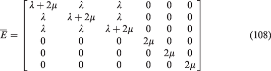
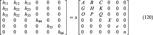
\bar{E} = [\begin{matrix} λ + 2 μ & λ & λ & 0 & 0 & 0 \\ λ & λ + 2 μ & λ & 0 & 0 & 0 \\ λ & λ & λ + 2 μ & 0 & 0 & 0 \\ 0 & 0 & 0 & 2 μ & 0 & 0 \\ 0 & 0 & 0 & 0 & 2 μ & 0 \\ 0 & 0 & 0 & 0 & 0 & 2 μ \end{matrix}]

(108)

The damaged/healed elasticity tensor is represented by the following 6 × 6 matrix for isotropic elasticity that includes the parameters of fabric tensors:

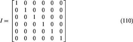
E = [\begin{matrix} (λ + 2 μ) m_{1}^{2 k} & λ m_{1}^{k} m_{2}^{k} & λ m_{1}^{k} m_{3}^{k} & 0 & 0 & 0 \\ λ m_{2}^{k} m_{1}^{k} & (λ + 2 μ) m_{2}^{2 k} & λ m_{2}^{k} m_{3}^{k} & 0 & 0 & 0 \\ λ m_{3}^{k} m_{1}^{k} & λ m_{3}^{k} m_{2}^{k} & (λ + 2 μ) m_{3}^{2 k} & 0 & 0 & 0 \\ 0 & 0 & 0 & 2 μ m_{2}^{k} m_{3}^{k} & 0 & 0 \\ 0 & 0 & 0 & 0 & 2 μ m_{3}^{k} m_{1}^{k} & 0 \\ 0 & 0 & 0 & 0 & 0 & 2 μ m_{1}^{k} m_{2}^{k} \end{matrix}]

(109)

The 6 × 6 identity tensor is written as follows in matrix form:

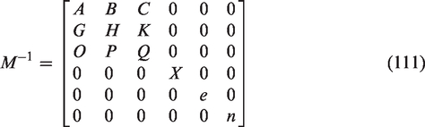
I = [\begin{array}{l} 1 & 0 & 0 & 0 & 0 & 0 \\ 0 & 1 & 0 & 0 & 0 & 0 \\ 0 & 0 & 1 & 0 & 0 & 0 \\ 0 & 0 & 0 & 1 & 0 & 0 \\ 0 & 0 & 0 & 0 & 1 & 0 \\ 0 & 0 & 0 & 0 & 0 & 1 \end{array}]

(110)

The 6 × 6 inverse tensors for damage and healing are represented in general by the following two matrices for the cases of isotropic damage and isotropic healing, respectively:

M^{- 1} = [\begin{array}{l} A & B & C & 0 & 0 & 0 \\ G & H & K & 0 & 0 & 0 \\ O & P & Q & 0 & 0 & 0 \\ 0 & 0 & 0 & X & 0 & 0 \\ 0 & 0 & 0 & 0 & e & 0 \\ 0 & 0 & 0 & 0 & 0 & n \end{array}]

(111)

H^{- 1} = [\begin{array}{l} h_{11} & h_{12} & h_{13} & 0 & 0 & 0 \\ h_{21} & h_{22} & h_{23} & 0 & 0 & 0 \\ h_{31} & h_{32} & h_{33} & 0 & 0 & 0 \\ 0 & 0 & 0 & h_{44} & 0 & 0 \\ 0 & 0 & 0 & 0 & h_{55} & 0 \\ 0 & 0 & 0 & 0 & 0 & h_{66} \end{array}]

(112)

For the case of the hypothesis of strain equivalence, one substitutes the above matrices into equation (5) which is reproduced below:

[M^{- 1} + (I - M^{- 1}) H^{- 1}] \bar{E} = E

(113)

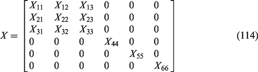
The left-hand-side of equation (113) is denoted by the matrix X. This matrix can be represented in general by the following form:

X = [\begin{array}{l} X_{11} & X_{12} & X_{13} & 0 & 0 & 0 \\ X_{21} & X_{22} & X_{23} & 0 & 0 & 0 \\ X_{31} & X_{32} & X_{33} & 0 & 0 & 0 \\ 0 & 0 & 0 & X_{44} & 0 & 0 \\ 0 & 0 & 0 & 0 & X_{55} & 0 \\ 0 & 0 & 0 & 0 & 0 & X_{66} \end{array}]

(114)

where the elements of the matrix X are presented explicitly in Appendix 3. These equations in the appendix form explicit relations between the elements of the damage tensor, the healing tensor, and fabric tensors. They apply for the case of isotropic elasticity for the hypothesis of strain equivalence.

Next, one presents the equations for isotropic elasticity for the hypothesis of elastic energy equivalence. For this purpose, equation (7) is reproduced below:

[M^{- 1} + (I - M^{- 1}) H^{- 1}] \bar{E} {[M^{- 1} + (I - M^{- 1}) H^{- 1}]}^{T} = E

(115)

Substituting the various matrices of isotropic elasticity that appear at the beginning of this section into equation (115), and labelling the left-hand-side of this equation as the matrix Y. This 6 × 6 matrix is represented in general as follows:

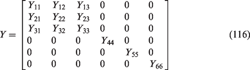
Y = [\begin{array}{l} Y_{11} & Y_{12} & Y_{13} & 0 & 0 & 0 \\ Y_{21} & Y_{22} & Y_{23} & 0 & 0 & 0 \\ Y_{31} & Y_{32} & Y_{33} & 0 & 0 & 0 \\ 0 & 0 & 0 & Y_{44} & 0 & 0 \\ 0 & 0 & 0 & 0 & Y_{55} & 0 \\ 0 & 0 & 0 & 0 & 0 & Y_{66} \end{array}]

(116)

The elements of the matrix Y are too complicated to list here. However, only the first element Y₁₁ is shown in Appendix 4. As can be seen from this appendix, the elements are too long and complicated. However, they are available with the authors and can be provided upon request.

As can be seen from the equations in Appendix 3 and Appendix 4, the relations between the components of the damage tensor, the healing tensor, and fabric tensors are too complicated for the case of isotropic elasticity. Therefore, no numerical example is presented in this case.

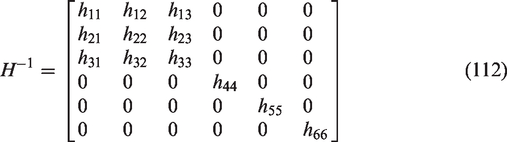
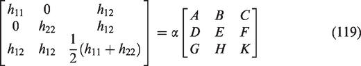
Finally, the full 6 × 6 matrix representation of the fourth-rank damage effect tensor M is shown in its entirety in Appendix 5. This matrix representation is taken from the previous work of the authors (Voyiadjis and Kattan, 1992, 2006).

Experimental results

Before one proceeds with the experimental setup and results, the reader needs to be aware of the following four issues in this work relating to theory vs. experiment. These issues may complicate matters and make comparison with experiments an impossibility.

The theory has been developed for damage and healing but the experiments in this part have been conducted to include damage with no healing.

The theory has been developed for metals and homogeneous materials but the experiments have been conducted on composite materials.

The theory has been developed for elastic materials but the experiments may include inelastic behavior.

An assumption is made that healing constitutes a maximum of about 10% of damage. This assumption is implemented using two different methods, called here Method I and Method II.

Since there is only one tensorial equation with three variables (for each hypothesis), namely fabric tensors, healing tensors, and damage tensors, the equation cannot be solved as is. One needs to make an assumption in order to solve for one of these variables in terms of the others. The assumption is made that healing constitutes roughly about 10% of damage (see item 4 above). This assumption can be implemented using two methods which are called here Method I and Method II.

Composite material specimens

The composite samples that are investigated experimentally are titanium aluminide (Ti-14Al-21Nb( $α_{2}$ )) composite reinforced with continuous SiC (SCS–6) fibers. The details of these composite materials are obtained from Voyiadjis and Almasri (2007).

Two laminate setups are considered: [0/90]_s and [±45]_s manufactured as detailed in the two references above. Four plies are included in each layup configuration. The details of the manufacturing and fabrication process are described by Voyiadjis et al. (1995) and Voyiadjis and Almasri (2007). Each one of the two laminate configurations was machined to produce six tensile test specimens as shown in Figure 7.

Figure 7.

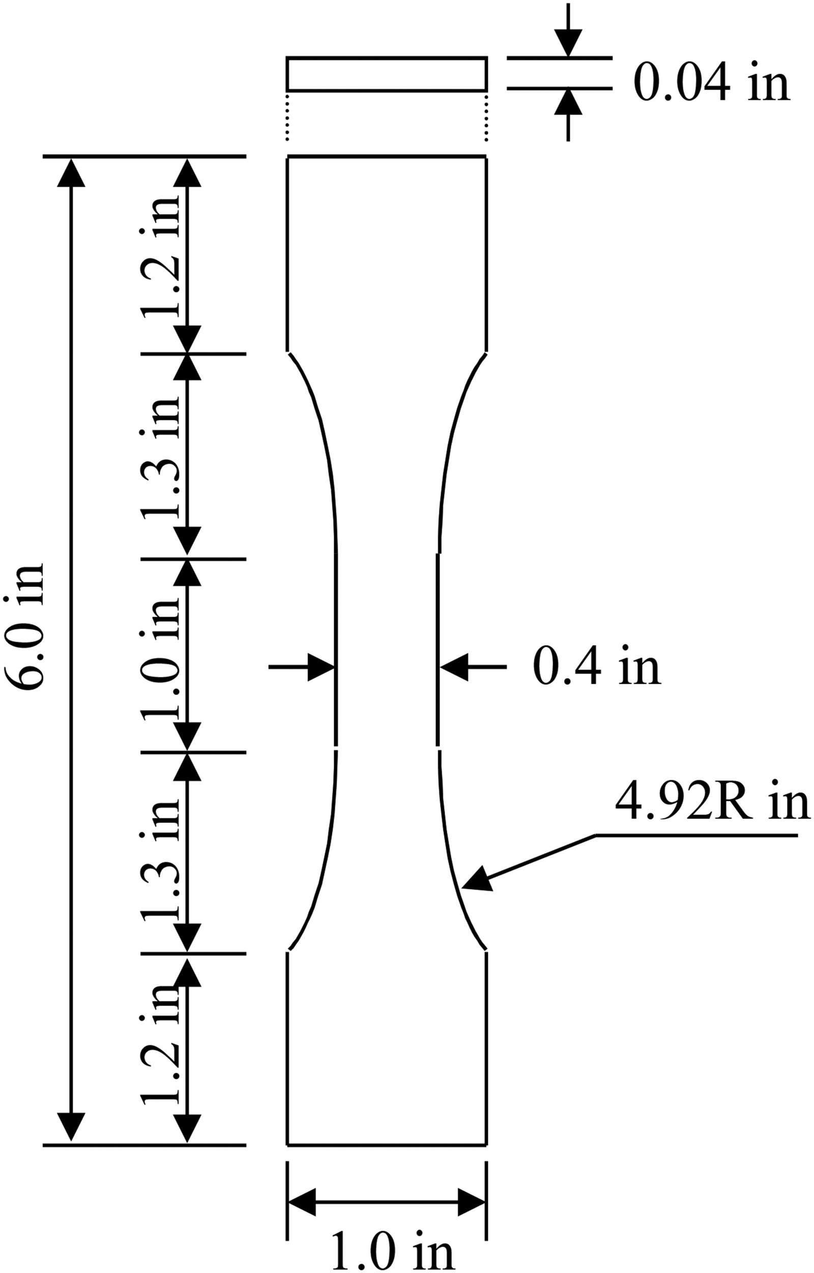
The typical tensile specimen for the composite material.

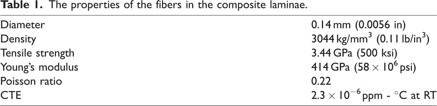
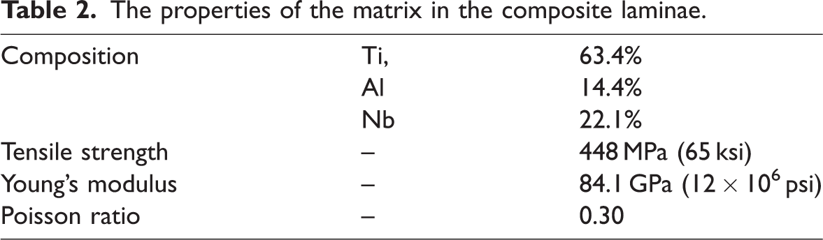
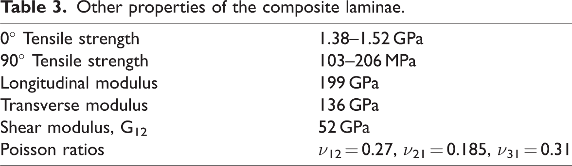
One specimen of each layup is tested up to failure. The other specimens are loaded up to 90, 85, 80, 75, and 70% of the failure load. The details of the characterization and investigation of the various micro-crack distributions in the cross-sections of the specimens are described by Voyiadjis and Almasri (2007). The material properties used in the experiments are listed in Tables 1, 2, and 3.

SEM images

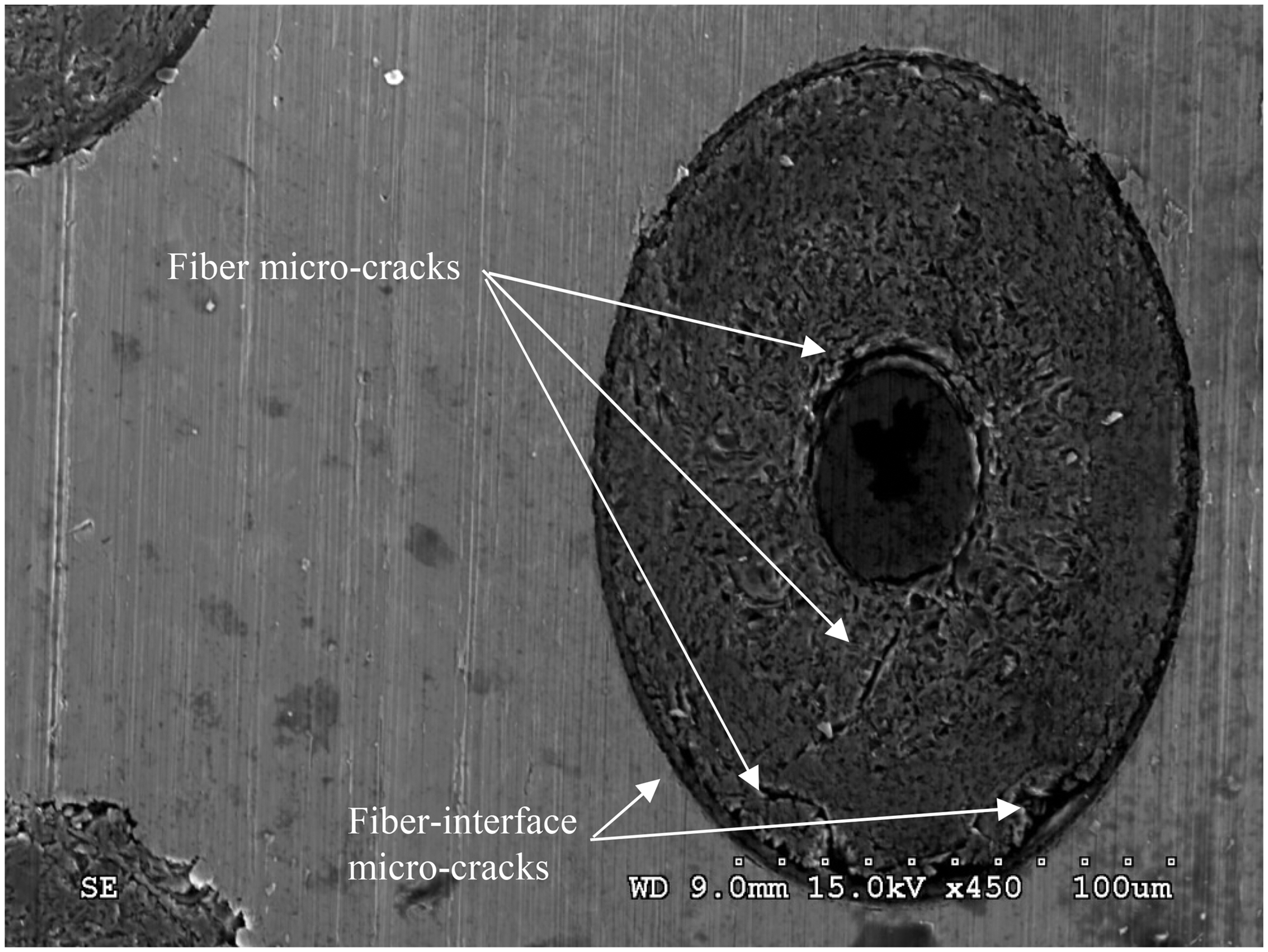
Various SEM images are shown in Figures 8 to 11 of the fiber and fiber-interface micro-cracks for both specimens. These images are reproduced from the work of Voyiadjis and Almasri (2007) with permission. The various micro-cracks are clearly evident in these images.

Figure 8.

The fiber micro-cracks with a 85% load [±45]_s sample (Voyiadjis and Almasri (2007).

Figure 9.

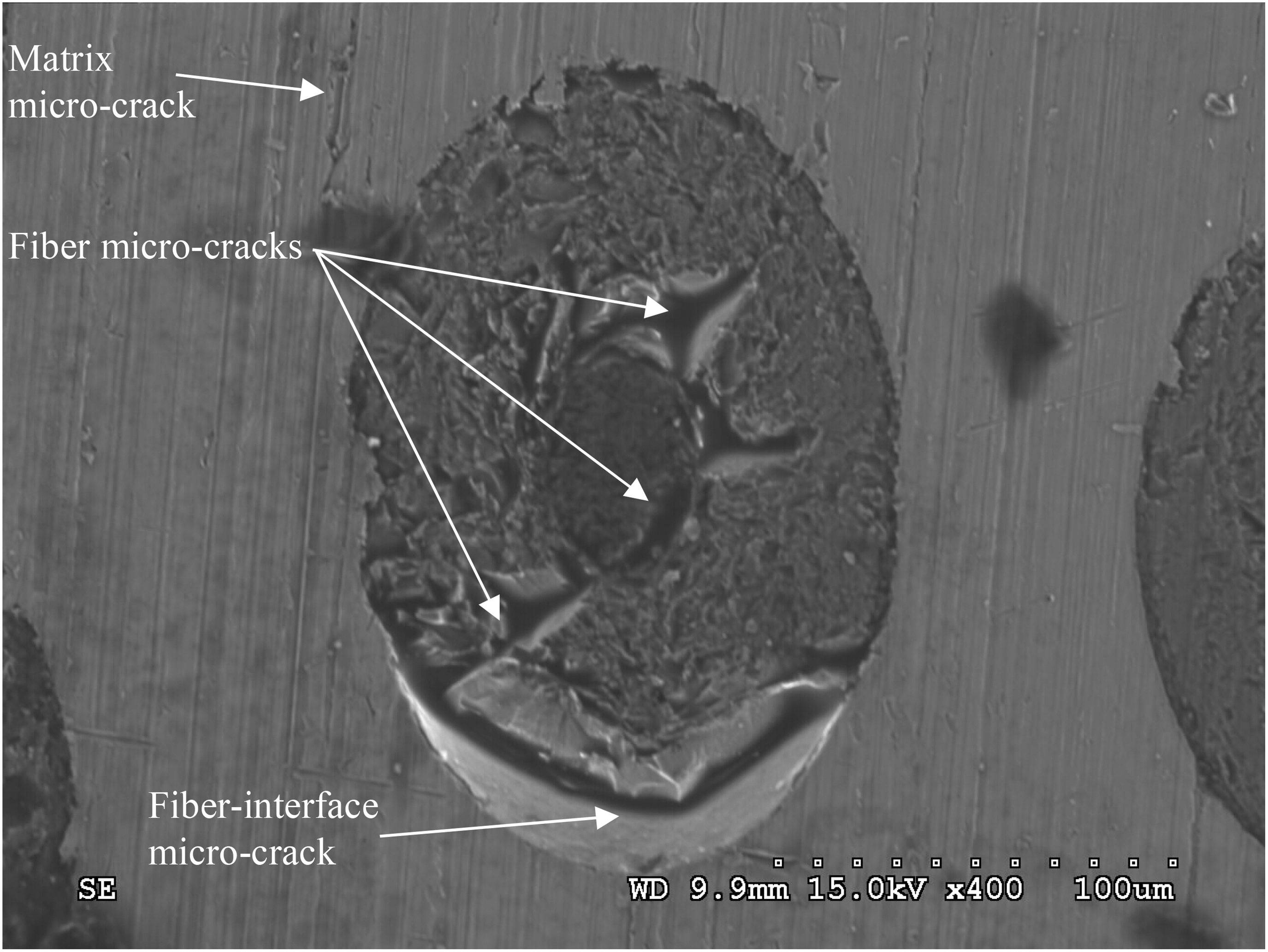
The fiber micro-cracks with a 90% load [±45]_s sample (Voyiadjis and Almasri (2007).

Figure 10.

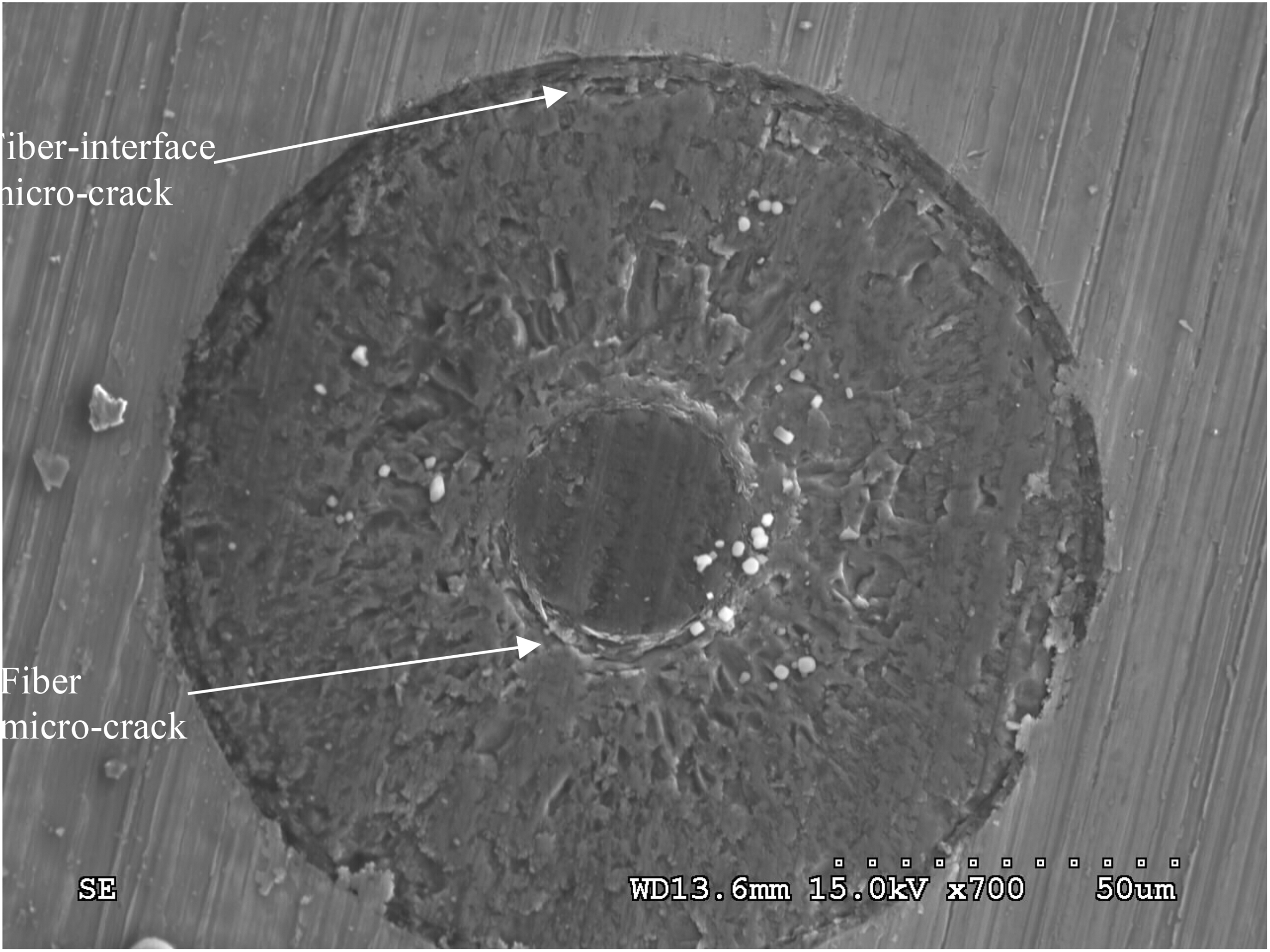
The fiber interface micro-cracks with a 75% load [0/90]_s sample (Voyiadjis and Almasri (2007).

Figure 11.

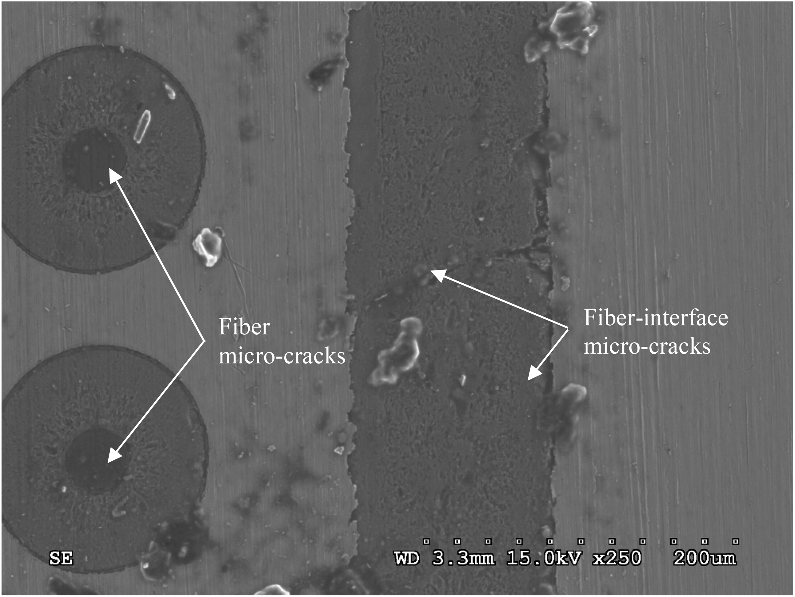
The fiber micro-cracks with a 100% load [0/90]_s sample (Voyiadjis and Almasri (2007).

Figures 12 to 15 show the evolution of micro-cracks for both specimens. These figures are generated from the formulas of fabric tensors shown in Appendix 2. These figures are taken based on the work of Voyiadjis and Almasri (2007).

Figure 12.

A rose diagram or a polar plot showing the evolution of fiber micro-cracks using a tenth order fabric tensor approximation of the [±45]_s laminate (Voyiadjis and Almasri (2007).

Figure 13.

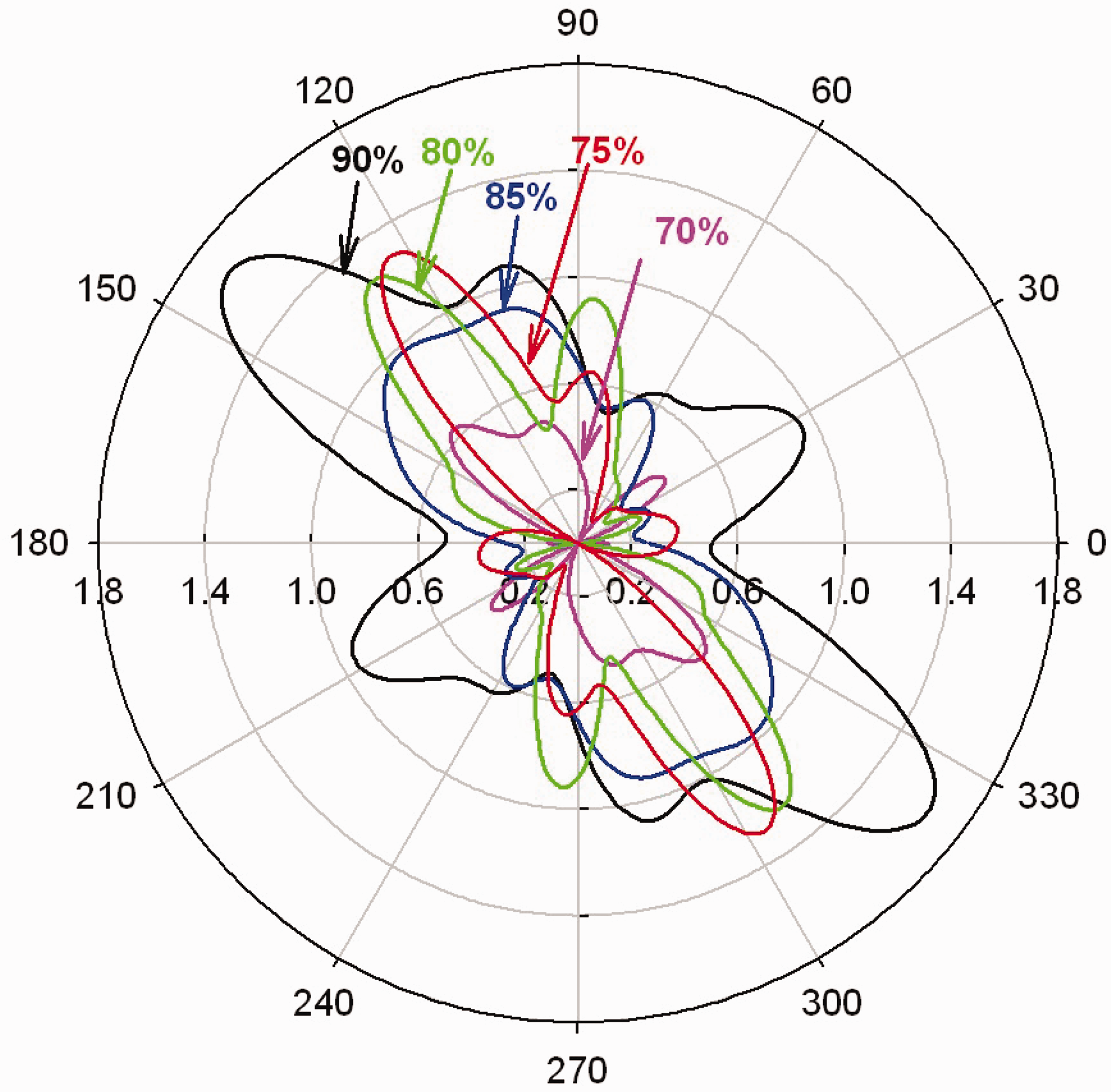
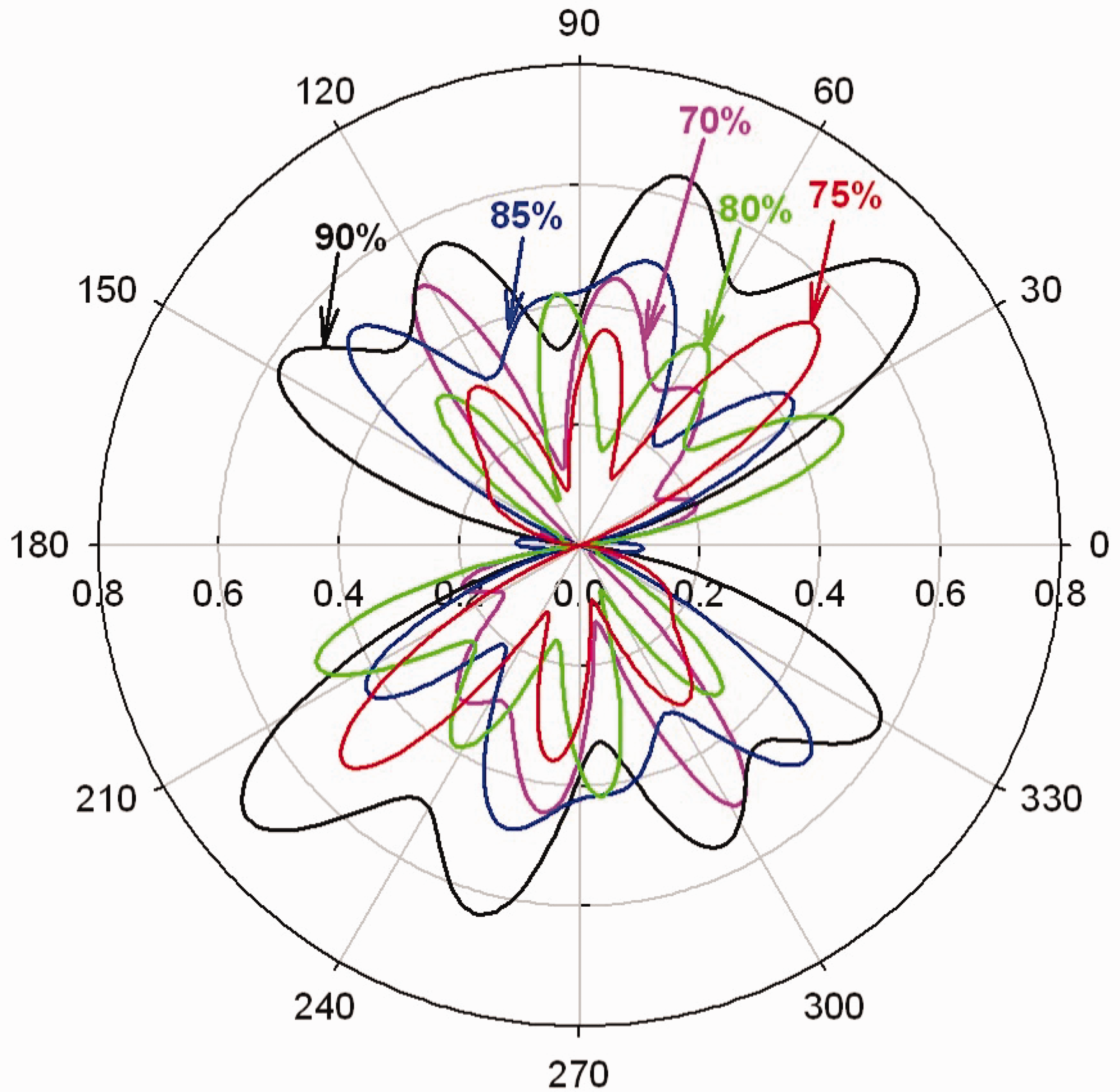
A rose diagram or a polar plot showing the evolution of fiber-interface micro-cracks using a tenth order fabric tensor approximation of the [±45]_s laminate (Voyiadjis and Almasri (2007).

Figure 14.

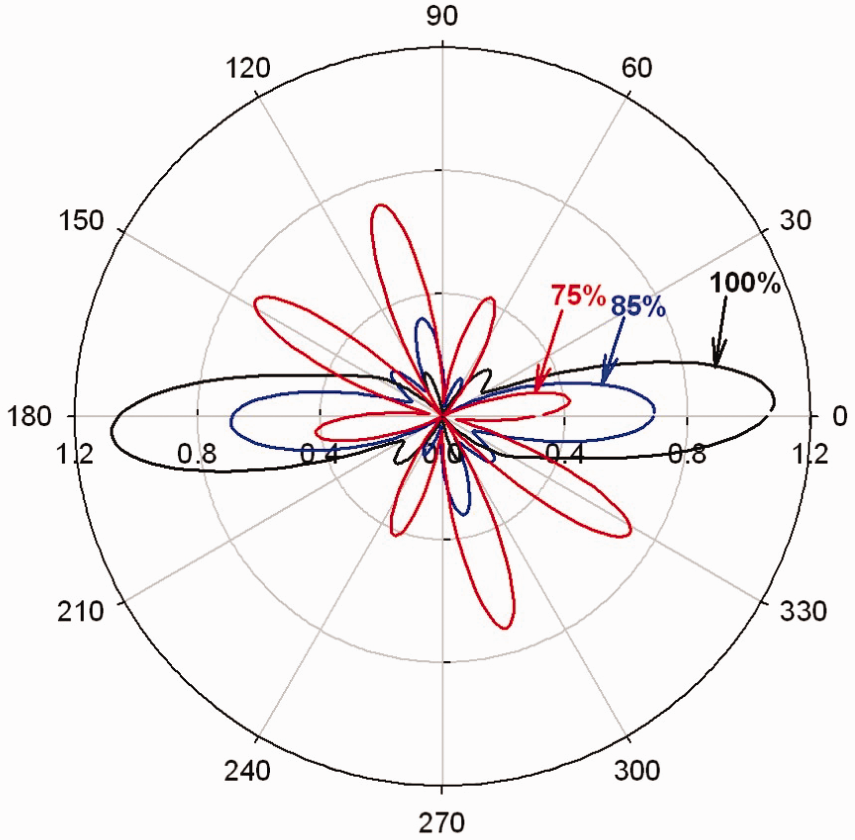
A rose diagram or a polar plot showing the evolution of fiber micro-cracks using a tenth order fabric tensor approximation of the [0/90]_s laminate (Voyiadjis and Almasri (2007)).

Figure 15.

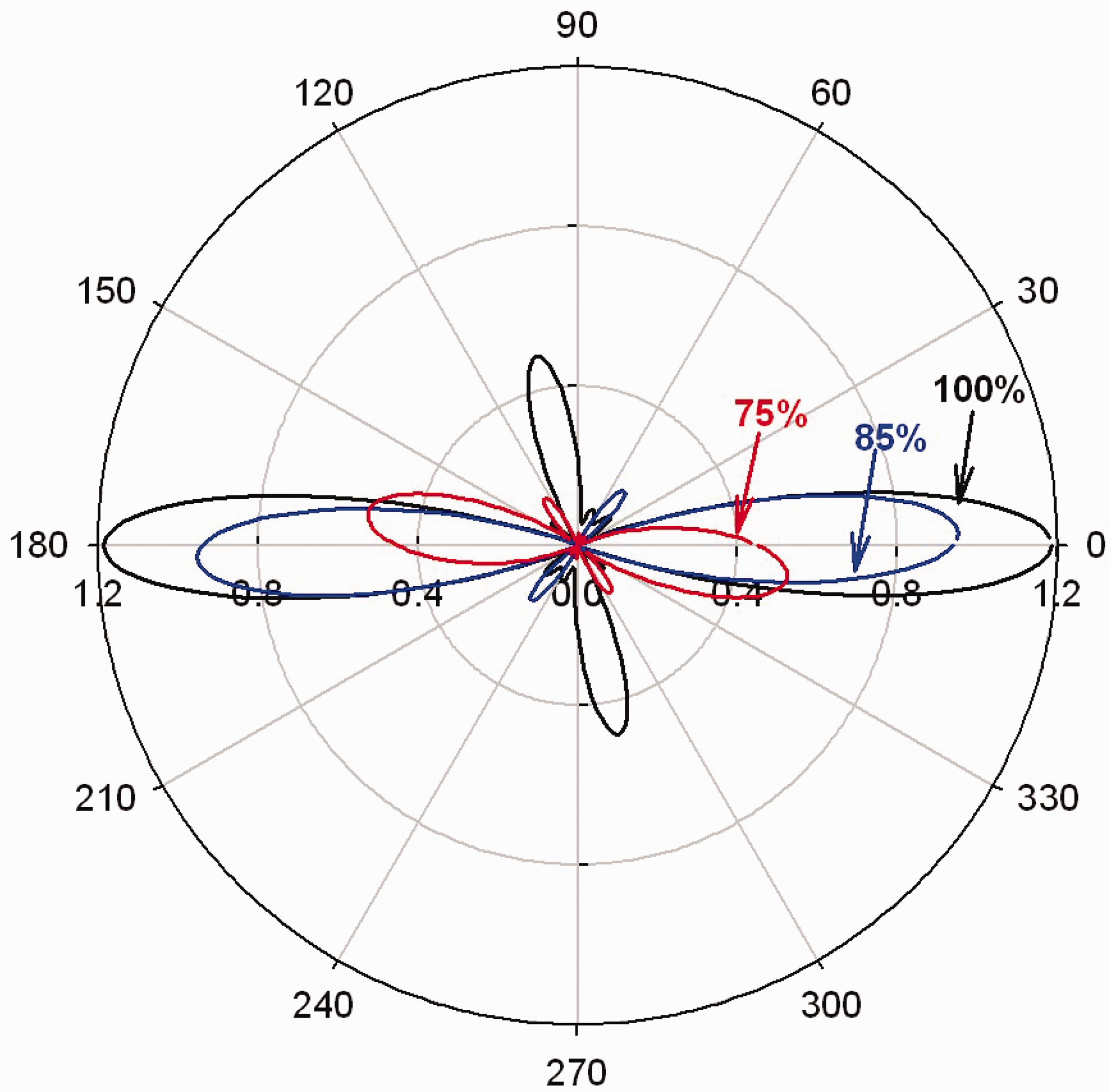
A rose diagram or a polar plot showing the evolution of fiber-interface micro-cracks using a tenth order fabric tensor approximation of the [0/90]_s laminate (Voyiadjis and Almasri (2007)).

Relationship between damage and healing

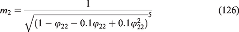
In this section, the relationship between the damage tensor and healing tensor is illustrated. As we have mentioned before, it is assumed that healing constitutes 10% of damage. In general, a general relationship can be assumed in terms of a factor $α$ and this factor can be later assigned the value of 10% or 0.1. This is accomplished through microcrack interactions, consequently, arresting further damage (micro-cracks) and producing partial healing through micro-crack partial closure. As mentioned before also, there are two methods in which this can be achieved. These methods are termed Method I and Method II below.

Method I is written in equation form as follows:

h_{i j} = α φ_{i j}

(117)

The above method assumes the relationship is between the elements of each tensor respectively. Alternatively, Method II is defined in terms of the whole tensor as follows:

H^{- 1} = α M^{- 1}

(118)

It is seen from equations (117) and (118) that the two methods are different and they will prove to provide different results. In terms of component form, Method II can be written in the following form for the case of plane stress or plane strain:

[\begin{matrix} h_{11} & 0 & h_{12} \\ 0 & h_{22} & h_{12} \\ h_{12} & h_{12} & \frac{1}{2} (h_{11} + h_{22}) \end{matrix}] = α [\begin{array}{l} A & B & C \\ D & E & F \\ G & H & K \end{array}]

(119)

In the case of isotropic elasticity, Method II can be written as follows:

[\begin{array}{l} h_{11} & h_{12} & h_{13} & 0 & 0 & 0 \\ h_{21} & h_{22} & h_{23} & 0 & 0 & 0 \\ h_{31} & h_{32} & h_{33} & 0 & 0 & 0 \\ 0 & 0 & 0 & h_{44} & 0 & 0 \\ 0 & 0 & 0 & 0 & h_{55} & 0 \\ 0 & 0 & 0 & 0 & 0 & h_{66} \end{array}] = α [\begin{array}{l} A & B & C & 0 & 0 & 0 \\ G & H & K & 0 & 0 & 0 \\ O & P & Q & 0 & 0 & 0 \\ 0 & 0 & 0 & X & 0 & 0 \\ 0 & 0 & 0 & 0 & e & 0 \\ 0 & 0 & 0 & 0 & 0 & n \end{array}]

(120)

For the hypothesis of strain equivalence, Method I takes the following form:

h_{11} = α φ_{11}

(121)

h_{22} = α φ_{22}

(122)

Substituting the above relations into the appropriate relation for the hypothesis of strain equivalence, one obtains the following relations:

m_{1} = \frac{1}{{\sqrt{(1 - φ_{11} + 0.1 φ_{11}^{2})}}^{5}}

(123)

m_{2} = \frac{1}{{\sqrt{(1 - φ_{22} + 0.1 φ_{22}^{2})}}^{5}}

(124)

For Method II and using the hypothesis of strain equivalence, and after going through the derivations (not shown here), one obtains the following relations:

m_{1} = \frac{1}{{\sqrt{(1 - φ_{11} - 0.1 φ_{11} + 0.1 φ_{11}^{2})}}^{5}}

(125)

m_{2} = \frac{1}{{\sqrt{(1 - φ_{22} - 0.1 φ_{22} + 0.1 φ_{22}^{2})}}^{5}}

(126)

Next, one presents the derived relationships for the hypothesis of elastic energy equivalence. For Method I, the following are obtained:

m_{1} = \frac{1}{{(0.1 φ_{11}^{2} + 1 - φ_{11})}^{5}}

(127)

m_{2} = \frac{1}{{(0.1 φ_{22}^{2} + 1 - φ_{22})}^{5}}

(128)

For Method II and for this last hypothesis, the following relations are obtained:

m_{1} = \frac{1}{{[0.1 φ_{11} (1 - φ_{11}) + 1 - φ_{11}]}^{5}}

(129)

m_{2} = \frac{1}{{[0.1 φ_{22} (1 - φ_{22}) + 1 - φ_{22}]}^{5}}

(130)

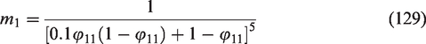
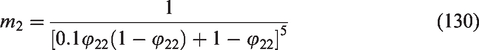
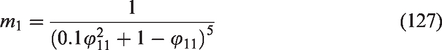
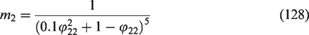
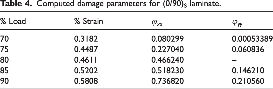
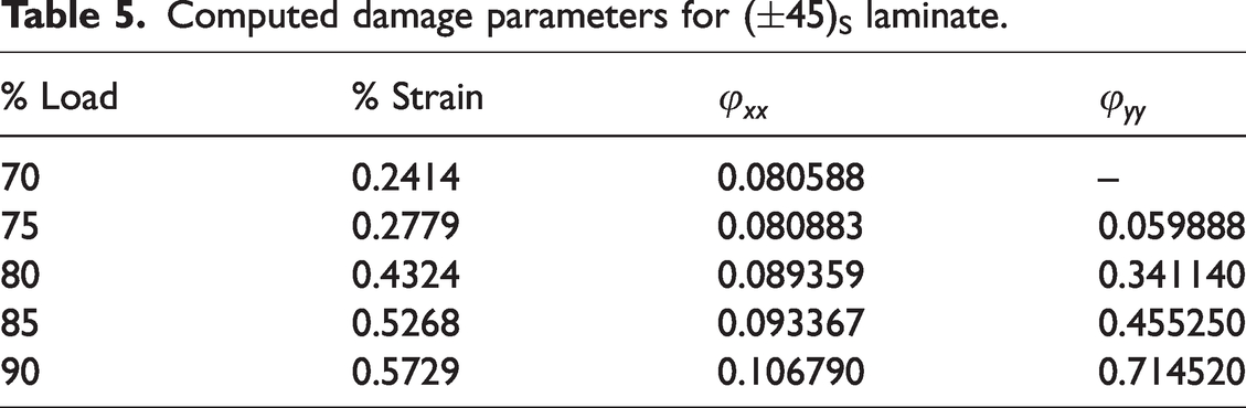
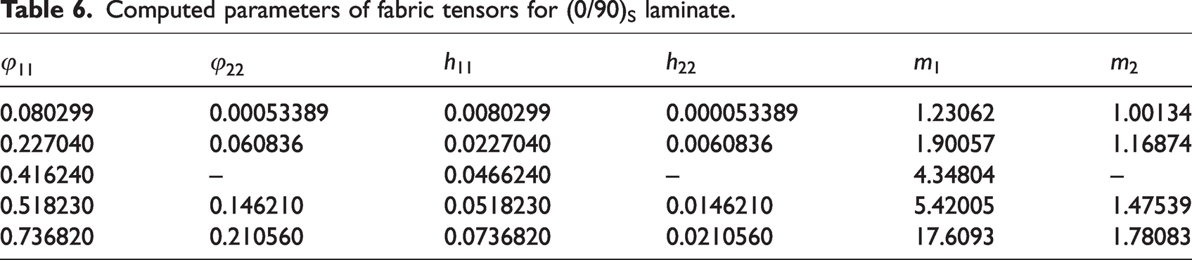
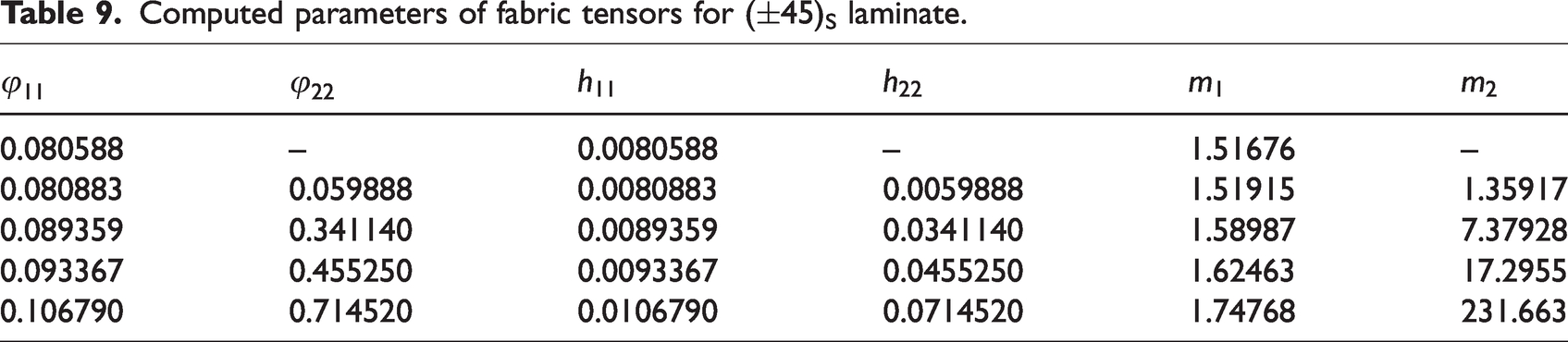
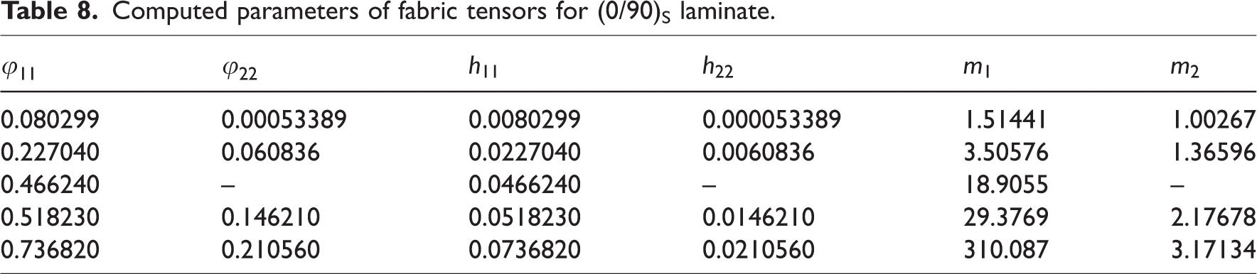
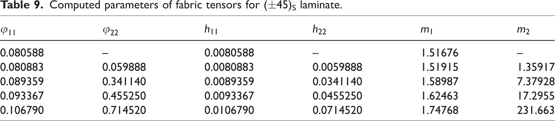
Finally, the following tables present the computed damage parameters and fabric tensor parameters for both laminate specimens tested. Specifically, Tables 4 and 5 present the values of the damage tensor components for each laminate. Tables 6 and 7 present the values of the fabric tensor parameters for each laminate for the hypothesis of strain equivalence while Tables 8 and 9 present those values for the hypothesis of elastic energy equivalence. The values of the fabric tensor parameters in Tables 6 to 9 were calculated based on equations (123) to (130) above.

Table 1.

The properties of the fibers in the composite laminae.

Diameter	0.14 mm (0.0056 in)
Density	3044 kg/mm³ (0.11 lb/in³)
Tensile strength	3.44 GPa (500 ksi)
Young’s modulus	414 GPa (58 × 10⁶ psi)
Poisson ratio	0.22
CTE	2.3 × 10⁻⁶ppm - °C at RT

Table 2.

The properties of the matrix in the composite laminae.

Composition	Ti,	63.4%
	Al	14.4%
	Nb	22.1%
Tensile strength	–	448 MPa (65 ksi)
Young’s modulus	–	84.1 GPa (12 × 10⁶ psi)
Poisson ratio	–	0.30

Table 3.

Other properties of the composite laminae.

0° Tensile strength	1.38–1.52 GPa
90° Tensile strength	103–206 MPa
Longitudinal modulus	199 GPa
Transverse modulus	136 GPa
Shear modulus, G₁₂	52 GPa
Poisson ratios	ν₁₂ = 0.27, ν₂₁ = 0.185, ν₃₁ = 0.31

Table 4.

Computed damage parameters for (0/90)_S laminate.

% Load	% Strain	$φ_{x x}$	$φ_{y y}$
70	0.3182	0.080299	0.00053389
75	0.4487	0.227040	0.060836
80	0.4611	0.466240	–
85	0.5202	0.518230	0.146210
90	0.5808	0.736820	0.210560

Table 5.

Computed damage parameters for ( $\pm$ 45)_S laminate.

% Load	% Strain	$φ_{x x}$	$φ_{y y}$
70	0.2414	0.080588	–
75	0.2779	0.080883	0.059888
80	0.4324	0.089359	0.341140
85	0.5268	0.093367	0.455250
90	0.5729	0.106790	0.714520

Table 6.

Computed parameters of fabric tensors for (0/90)_S laminate.

$φ_{11}$	$φ_{22}$	$h_{11}$	$h_{22}$	$m_{1}$	$m_{2}$
0.080299	0.00053389	0.0080299	0.000053389	1.23062	1.00134
0.227040	0.060836	0.0227040	0.0060836	1.90057	1.16874
0.416240	–	0.0466240	–	4.34804	–
0.518230	0.146210	0.0518230	0.0146210	5.42005	1.47539
0.736820	0.210560	0.0736820	0.0210560	17.6093	1.78083

Table 7.

Computed parameters of fabric tensors for ( $\pm$ 45)_S laminate.

$φ_{11}$	$φ_{22}$	$h_{11}$	$h_{22}$	$m_{1}$	$m_{2}$
0.080588	–	0.0080588	–	1.23157	–
0.080883	0.059888	0.0080883	0.0059888	1.23254	1.16583
0.089359	0.341140	0.0089359	0.0341140	1.26090	2.71648
0.093367	0.455250	0.0093367	0.0455250	1.27461	4.15878
0.106790	0.714520	0.0106790	0.0714520	1.32200	15.2205

Table 8.

Computed parameters of fabric tensors for (0/90)_S laminate.

$φ_{11}$	$φ_{22}$	$h_{11}$	$h_{22}$	$m_{1}$	$m_{2}$
0.080299	0.00053389	0.0080299	0.000053389	1.51441	1.00267
0.227040	0.060836	0.0227040	0.0060836	3.50576	1.36596
0.466240	–	0.0466240	–	18.9055	–
0.518230	0.146210	0.0518230	0.0146210	29.3769	2.17678
0.736820	0.210560	0.0736820	0.0210560	310.087	3.17134

Table 9.

Computed parameters of fabric tensors for ( $\pm$ 45)_S laminate.

$φ_{11}$	$φ_{22}$	$h_{11}$	$h_{22}$	$m_{1}$	$m_{2}$
0.080588	–	0.0080588	–	1.51676	–
0.080883	0.059888	0.0080883	0.0059888	1.51915	1.35917
0.089359	0.341140	0.0089359	0.0341140	1.58987	7.37928
0.093367	0.455250	0.0093367	0.0455250	1.62463	17.2955
0.106790	0.714520	0.0106790	0.0714520	1.74768	231.663

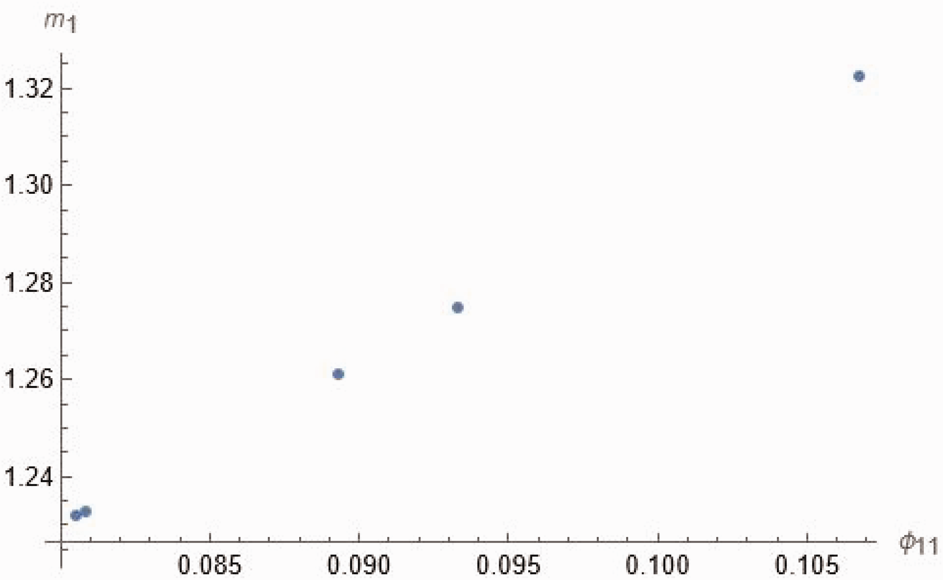
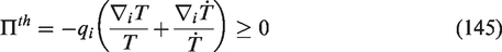
The values of fabric tensors parameters in Table 6 are shown graphically in Figure 16. It is shown in this figure that the fabric tensor parameter reaches a maximum value of about 15. Similarly, the values of fabric tensor parameters of Table 7 are shown graphically in Figure 17. These values reach a maximum value of 1.32. It seems that the second specimen obtains relatively smaller values of the fabric tensors.

Figure 16.

Plot showing relationship between damage tensor component and fabric tensor parameter for the hypothesis of strain equivalence for the [0/90]_s laminate.

Figure 17.

Plot showing relationship between damage tensor component and fabric tensor parameter for the hypothesis of strain equivalence for the [±45]_s laminate.

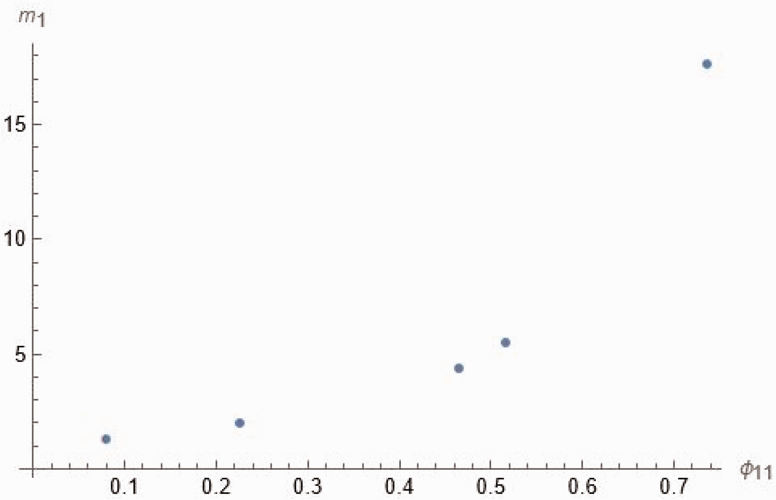
Finally, the fabric tensor values of Table 8 are shown graphically in Figure 18. It is seen that these values reach a maximum value of 300. On the other hand, those maximum values for the other specimen reach a maximum value of 1.75 as shown in Table 9 and Figure 19. Thus, the second specimen again obtains smaller values of the fabric tensor parameters.

Figure 18.

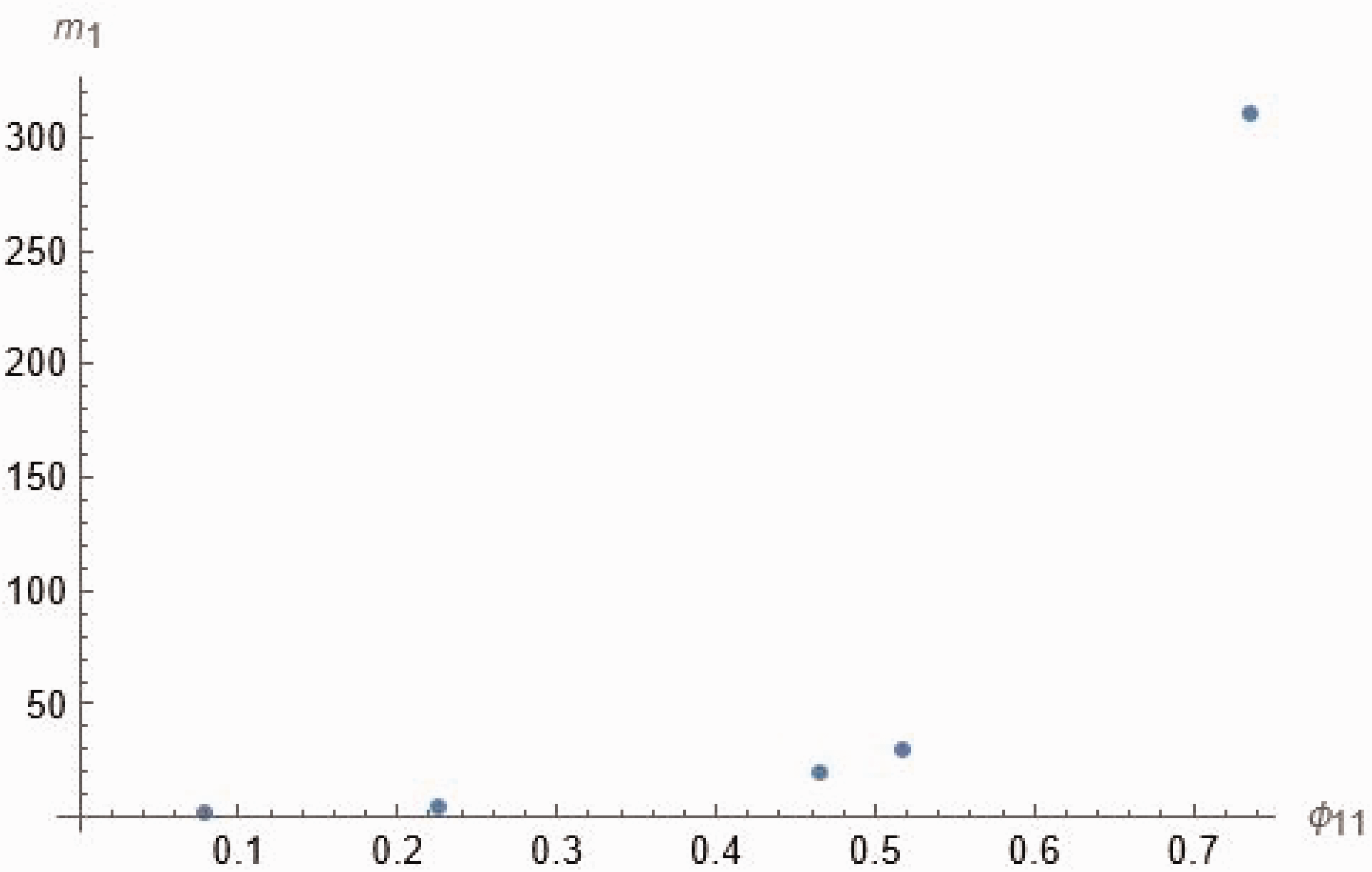
Plot showing relationship between damage tensor component and fabric tensor parameter for the hypothesis of elastic energy equivalence for the [0/90]s laminate.

Figure 19.

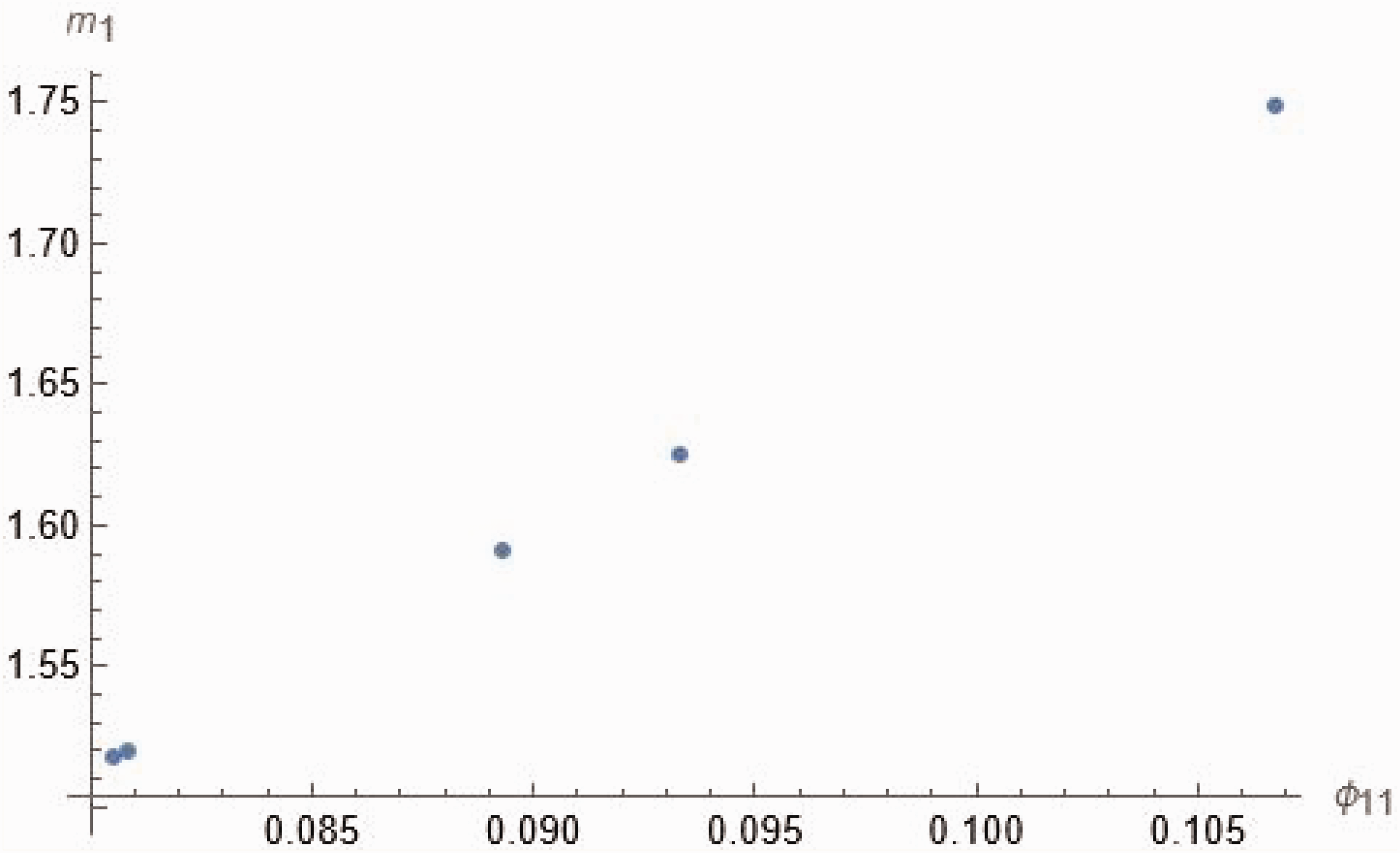
Plot showing relationship between damage tensor component and fabric tensor parameter for the hypothesis of elastic energy equivalence for the [±45]s laminate.

It should be noted that much higher values are obtained for fabric tensor parameters when the hypothesis of elastic energy equivalence is used. The more simplistic hypothesis of strain equivalence has smaller values of the fabric tensor parameters.

Thermodynamics of damage and healing evolution

In this section, the mechanics of thermal damage elasticity is studied. Damage and healing evolution is investigated based on sound thermodynamics pricniples The various independent variables considered are the strain tensor $ε$ (completely elastic), the absolute temperature $T$ , the temperature gradient vector $\nabla_{i} T$ , and certain internal state variables $N_{k} (k = 1, 2, 3)$ . In this thermodynamics analysis, one assumes small displacements and strains. Therefore, the Helmholtz free energy density function $Ψ$ can be presented in the following manner (Coleman and Gurtin, 1967; Doghri, 2000; Lemaitre and Chaboche, 1990; Lubliner, 1990; Voyiadjis and Kattan, 1999):

Ψ = \tilde{Ψ} (ε_{ij}, T, \nabla_{i} T, N_{k})

(131)

In order to characterize the different damage and healing processes, certain internal state variables $N_{k}$ representing either a scalar or a tensorial variable are used such that:

N_{k} = {\tilde{N}}_{k} (Ξ_{n})

(132)

where

Ξ_{n}

is a collection of damage/healing internal state variables. This is usually written in the following general form:

Ξ_{n} = {\tilde{Ξ}}_{n} (r, Γ_{ijkl}, M_{ijkl}, H_{ijkl})

(133)

where

r

represents the accumulative damage,

Γ

denotes the flux of the residual stress, and M and H denote the fourth-rank damage tensor and fourth-rank healing tensor, respectively. These damage/healing internal state variables are introduced in the Helmholtz free energy density to give enough details of the various defects in order to characterize the micro-structural behavior.

It is important to find the evolution of these internal state variables and this is a crucial step in the constitutive modeling. This issue of evolution can be obtained using sound thermodynamics pricniples as is shown in this section. (See the references by Coleman and Gurtin, 1967; Doghri, 2000; Lemaitre and Chaboche, 1990; Lubliner, 1990; Voyiadjis and Kattan, 1999).

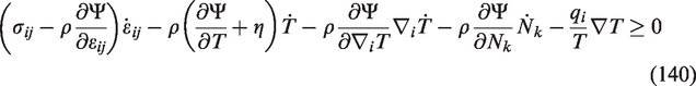
The Clausius-Duhem inequality is written in the following form:

σ_{i j} {\dot{ε}}_{i j} - ρ (\dot{Ψ} + η \dot{T}) - \frac{1}{T} q_{i} \nabla_{i} T \geq 0

(134)

where

ρ

η

, and

q

are the mass density, specific entropy, and the heat flux vector, respectively. Meanwhile, the relationship between

Ψ

, T, and

η

is given by:

Ψ = e - T η

(135)

where

e

is the internal energy density. The free energy density function is decomposed into two parts (one elastic and one damage) as follows:

\begin{array}{l} \tilde{Ψ} (ε_{i j}, T, \nabla_{i} T, N_{k}) = {\tilde{Ψ}}^{t e} (ε_{i j}, T, \nabla_{i} T, M_{ijkl}, H_{ijkl}) + {\tilde{Ψ}}^{t d} (T, \nabla_{i} T, r, Γ_{i j}, M_{ijkl}, H_{ijkl}) \end{array}

(136)

where

Ψ^{t e}

is the thermo-elastic stored energy while

Ψ^{t d}

is the energy stored due to material hardening due to the damage processes.

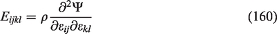
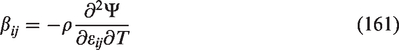
The time derivative of the free energy density function of equation (131) with respect to its internal state variables is given by:

\dot{Ψ} = \frac{\partial Ψ}{\partial ε_{i j}} {\dot{ε}}_{i j} + \frac{\partial Ψ}{\partial T} \dot{T} + \frac{\partial Ψ}{\partial \nabla_{i} T} \nabla_{i} \dot{T} + \frac{\partial Ψ}{\partial N_{k}} {\dot{N}}_{k}

(137)

where (from equation (132)):

\frac{\partial Ψ}{\partial N_{k}} {\dot{N}}_{k} = \frac{\partial Ψ}{\partial Ξ_{n}} {\dot{Ξ}}_{n}

(138)

with (from equation (133)):

\frac{\partial Ψ}{\partial Ξ_{n}} {\dot{Ξ}}_{n} = \frac{\partial Ψ}{\partial r} \dot{r} + \frac{\partial Ψ}{\partial Γ_{ijkl}} {\dot{Γ}}_{ijkl} + \frac{\partial Ψ}{\partial M_{ijkl}} {\dot{M}}_{ijkl} + \frac{\partial Ψ}{\partial H_{ijkl}} {\dot{H}}_{ijkl}

(139)

Next one substitutes the rate of the Helmholtz free energy density (equation (137)) into the Clausius-Duhem inequality (equation (134)) to obtain the following thermodynamic constraint:

(σ_{i j} - ρ \frac{\partial Ψ}{\partial ε_{i j}}) {\dot{ε}}_{i j} - ρ (\frac{\partial Ψ}{\partial T} + η) \dot{T} - ρ \frac{\partial Ψ}{\partial \nabla_{i} T} \nabla_{i} \dot{T} - ρ \frac{\partial Ψ}{\partial N_{k}} {\dot{N}}_{k} - \frac{q_{i}}{T} \nabla T \geq 0

(140)

The following four thermodynamic state laws are then obtained from the above equation:

σ_{i j} = ρ \frac{\partial Ψ}{\partial ε_{i j}}

(140.1)

η= - \frac{\partial Ψ}{\partial T}

(140.2)

\frac{q_{i}}{\dot{T}} = ρ \frac{\partial Ψ}{\partial \nabla_{i} T}

(140.3)

Σ_{k} = ρ \frac{\partial Ψ}{\partial N_{k}} (k = 1, 2, 3)

(140.4)

where the above equations show the relationships between between the state variables and their associated thermodynamic conjugate forces. Note that the three thermodynamic conjugate forces

Σ_{k}

denote the following three quantities: K which is associated with r,

L_{ijkl}

which is associated with

Γ_{ijkl}

Y_{ijkl}

which is associated with

M_{ijkl}

and

U_{ijkl}

which is associated with

H_{ijkl}

. The conjugate forces K and L characterize the damage changes while the conjugate force U characterize the healing changes.

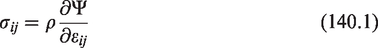
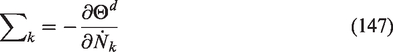
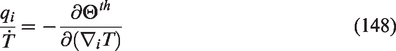
Substituting equations (140) into equation (139), one reduces the Clausius-Duhem inequality to show the fact that the dissipation energy 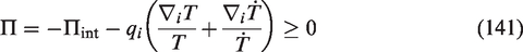$Π$ is positive:

Π = - Π_{int} - q_{i} (\frac{\nabla_{i} T}{T} + \frac{\nabla_{i} \dot{T}}{\dot{T}}) \geq 0

(141)

where the internal dissipation energy

Π_{int}

can be written as follows:

Π_{int} = \sum_{k = 1}^{3} \sum_{k} {\dot{N}}_{k} = K \dot{r} + H_{ijkl} {\dot{Γ}}_{ijkl} - Y_{ijkl} {\dot{M}}_{ijkl} + U_{ijkl} {\dot{H}}_{ijkl} \geq 0

(142)

The dissipation energy $Π$ may be decomposed as the summation of dissipations due to damage and thermal effects as follows:

Π = Π^{d} + Π^{t h}

(143)

where

Π^{d} = - K \dot{r} - H_{ijkl} {\dot{Γ}}_{ijkl} + Y_{ijkl} {\dot{M}}_{ijkl} - U_{ijkl} {\dot{H}}_{ijkl} \geq 0

(144)

Π^{t h} = - q_{i} (\frac{\nabla_{i} T}{T} + \frac{\nabla_{i} \dot{T}}{\dot{T}}) \geq 0

(145)

The dissipation processes of equations (144) and (145) imply the existence of the dissipation potential which is expressed as a continuous and convex scalar valued function of the flux variables as shown below:

Θ ({\dot{N}}_{k}, q_{i} / T) = Θ^{d} ({\dot{N}}_{k}) + Θ^{t h} (T, \nabla_{i} T)

(146)

The complementary laws are then expressed by the normality property as follows:

\sum_{k} = - \frac{\partial Θ^{d}}{\partial {\dot{N}}_{k}}

(147)

\frac{q_{i}}{\dot{T}} = - \frac{\partial Θ^{t h}}{\partial (\nabla_{i} T)}

(148)

Using the Legendre-Fenchel transformation of the dissipation potential $Θ$ , one can define the corresponding dual potential with respect to the force variables as follows:

\begin{array}{l} Θ^{*} (\sum_{k}, \nabla_{i} T) = Π (\sum_{k}, q_{i}; {\dot{N}}_{k}, T, \nabla_{i} T) - Θ ({\dot{N}}_{k}, T, \nabla_{i} T) \\ = Θ^{*^{d}} (\sum_{k}) + Θ^{*^{t h}} (T, \nabla_{i} T) \end{array}

(149)

Therefore, the evolution laws of the flux variables as a function of the dual variables can be presented as follows:

- {\dot{N}}_{k} = \frac{\partial Θ^{*^{d}}}{\partial \sum_{k}}

(150)

- \frac{\nabla_{i} T}{\dot{T}} = \frac{\partial Θ^{*^{t h}}}{\partial q_{i}}

(151)

The evolution formulas of the fourth-rank tensors of damage and healing M and H can be obtained using the calculus of several variables with the Lagrange multiplier ${\dot{λ}}^{d}$ . The dissipation function $Π^{d}$ (equations (143) and (144)) is used with the constraint $g = 0$ (Kattan and Voyiadjis, 1990, 1993, 2001b; Voyiadjis and Kattan, 1990, 1992, 1999) so that the following objective function is formed:

Ω = Π^{d} - {\dot{λ}}^{d} g

(152)

where

g

is the damage/healing surface (i.e. criterion). The maximization principle applied to the objective function of the equation above results in the following:

\frac{\partial Ω}{\partial Y_{ijkl}} = 0

(153.1)

\frac{\partial Ω}{\partial U_{ijkl}} = 0

(153.2)

Substitution of equation (152) into equations (153.1) and (153.2) along with equation (90) yields the thermodynamic formulas of the evolution of the damage tensor 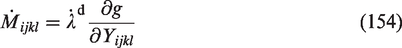$\dot{M}$ and evolution of the healing tensor $\dot{H}$ as follows:

{\dot{M}}_{ijkl} = {\dot{λ}}^{d} \frac{\partial g}{\partial Y_{ijkl}}

(154)

{\dot{H}}_{ijkl} = {\dot{λ}}^{h} \frac{\partial g}{\partial U_{ijkl}}

(155)

The above equation represents the evolution equation for the fourth-rank damage tensor $M$ and the fourth-rank healing tensor $H$ .

Next one defines the accumulative damage rate $\dot{r}$ as follows:

\dot{r} = \sqrt{{\dot{M}}_{ijkl} {\dot{M}}_{ijkl}}

(156)

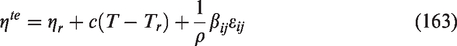
The thermo-elastic energy 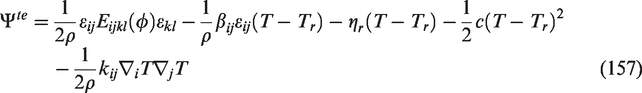$Ψ^{t e}$ can be written as follows:

Ψ^{t e} = \frac{1}{2 ρ} ε_{i j} E_{ijkl} (ϕ) ε_{k l} - \frac{1}{ρ} β_{i j} ε_{i j} (T - T_{r}) - η_{r} (T - T_{r}) - \frac{1}{2} c {(T - T_{r})}^{2} - \frac{1}{2 ρ} k_{i j} \nabla_{i} T \nabla_{j} T

(157)

On the other hand, the thermo-damage energy $Ψ^{t d}$ is written as follows:

ρ Ψ^{t d} = \frac{1}{2} a_{1} r^{2} V + \frac{1}{2} a_{2} Γ_{ijkl} Γ_{ijkl} V

(158)

where

E (φ)

is the fourth-rank damage elasticity tensor,

β

is the tangent conjugate tensor (Lubliner, 1990),

c

is the coefficient of thermal expansion,

η_{r}

is the reference entropy,

T_{r}

is the reference temperature,

a_{1}

and

a_{2}

are material-dependent constants which are considered independent of temperature,

k = k δ

is the heat conductivity second-rank tensor (

k

being the conductivity coefficient and

δ

is the Kronecker delta), and

V

is the homologous temperature defined as

V = 1 - {(T / T_{m})}^{n}

, where

T_{m}

is the melting temperature and

n

is the temperature softening component.

Next, one can study the constitutive equations of the model starting with the equation for the stress tensor shown below:

σ_{i j} = E_{ijkl} ε_{k l} - β_{i j} (T - T_{r})

(159)

where

E_{ijkl} = ρ \frac{\partial^{2} Ψ}{\partial ε_{i j} \partial ε_{k l}}

(160)

β_{i j} = - ρ \frac{\partial^{2} Ψ}{\partial ε_{i j} \partial T}

(161)

The constitutive equations for the entropy (equation (140.2)) can be written from the thermodynamic potential of equations (157) and (158) as follows:

η = η^{t e} + η^{t d}

(162)

where

η^{t e} = η_{r} + c (T - T_{r}) + \frac{1}{ρ} β_{i j} ε_{i j}

(163)

η^{t d} = \frac{1}{2 ρ} (a_{1} r^{2} + a_{2} Γ_{ijkl} Γ_{ijkl}) \frac{\partial V}{\partial T}

(164)

In the above equation, $\frac{\partial V}{\partial T}$ is given by:

\frac{\partial V}{\partial T} = \frac{n}{T_{m}} {(\frac{T}{T_{m}})}^{n - 1}

(165)

The constitutive equation for the heat flux vector $q$ can be obtained from equation (86.3) as follows:

q_{i} = - k_{i j} \nabla_{j} T

(166)

Next, one presents the damage potential function in the following form:

G = g + \frac{1}{2} h_{1} K^{2} + \frac{1}{2} h_{2} L_{ijkl} L_{ijkl}

(167)

where

h_{1}

and

h_{2}

are material constants, and

g

is the damage surface (criterion) defined as follows:

g = \sqrt{(Y_{ijkl} - L_{ijkl}) (Y_{ijkl} - L_{ijkl})} - l - K \leq 0

(168)

where the damage forces

Y

and

L

characterize damage evolution and damage kinematic hardening,

l

is the initial damage threshold as a function of temperature, while

K

is the damage isotropic hardening function.

The model response in the damage domain is then characterized by the Kuhn-Tucker complementary conditions as follows:

g \leq 0, {\dot{λ}}^{d} \geq 0, {\dot{λ}}^{d} g = 0

(169)

Next, the hardening evolution equation is derived as follows:

\dot{r} = {\dot{λ}}^{d} (1 - h_{1} K)

(170)

The evolution equations for the damage isotropic hardening function $K$ can be obtained by first making use of equation (170) and substituting it into the evolution law for $\dot{K}$ so that the following relation is obtained:

\dot{K} = a_{1} (1 - h_{1} K) {\dot{λ}}^{d} V

(171)

Furthermore, the evolution equation for the damage kinematic hardening parameter can be obtain by using equation (167) and substituting it into the evolution law of $\dot{Γ}$ while realizing that $\partial g / \partial L = - \partial g / \partial Y$ (clear from equation (168)), and using equation (100) to obtain:

{\dot{Γ}}_{ijkl} = {\dot{M}}_{ijkl} - h_{2} {\dot{λ}}^{d} L_{ijkl}

(172)

Finally, it can be easily seen that by substituting equation (172) into the evolution law of $\dot{L}$ , we may obtain the following relation:

{\dot{L}}_{ijkl} = (a_{2} {\dot{M}}_{ijkl} - h_{2} a_{2} {\dot{λ}}^{d} L_{ijkl}) V

(173)

Equations (170) to (173) are the governing evolution formulas for the various parameters involved in the damage process, healing process, and damage hardening.

Conclusion

The following conclusions are emphasized in this work. A link has been established between various fabric tensor parameters and damage and healing tensor components. Basically, the theory is developed for elastic materials. In addition, several examples are solved including plane stress, plane strain, and isotropic elasticity. For the case of isotropic elasticity it includes both isotropic damage and isotropic healing. The experiments that were conducted are for uniaxial tension on various composite laminae with different orientations. Lastly, the fabric tensor parameters for the experimental results are calculated and presented in both table and graph forms. Finally, the theory presented is thermodynamically consistent. A short section on thermodynamics is added in the previous section for this purpose.

In summary, the exact relationship between fabric tensors and the damage and healing tensors is established. This relationship was derived in the most general three-dimensional tensor form and applied to the examples of plane stress, plane strain, and isotropic elasticity. Finally, experimental observations have been studied and related to fabric tensor parameters.

In forthcoming papers, the authors will conduct experiments in damage and healing and demonstrate the physical basis of these complex but rigorous formulations. In general, a relationship can be assumed in terms of a factor $α$ and this factor is assigned in this work the value of 10% or 0.1. This is due to micro-crack interactions in these experiments, consequently, arresting further damage (micro-cracks) and producing partial healing through micro-crack partial closure in this case.

Footnotes

Declaration of conflicting interests

The author(s) declared no potential conflicts of interest with respect to the research, authorship, and/or publication of this article.

Funding

The author(s) received no financial support for the research, authorship, and/or publication of this article.

ORCID iD

George Z Voyiadjis

References

Betten

(1981) Damage tensors in continuum mechanics. Journal de mécanique théorique et appliquée 2: 13–32 (Presented at Euromech Colloqium 147 on Damage Mechanics, Paris-VI, Cachan, 22 September).

Betten

(1986) Applications of tensor functions to the formulation of constitutive equations involving damage and initial anisotropy. Engineering Fracture Mechanics 25(5–6): 573–584.

Cauvin

Testa

(1999) Damage mechanics: Basic variables in continuum theories. International Journal of Solids and Structures 36(5): 747–761.

Chow

Wang

(1987a) An anisotropic theory of elasticity for continuum damage mechanics. International Journal of Fracture 33(1): 3–16.

Chow

Wang

(1987b) An anisotropic theory of continuum damage mechanics for ductile fracture. Engineering Fracture Mechanics 27(5): 547–558.

Chow

Wang

(1988) Ductile fracture characterization with an anisotropic continuum damage theory. Engineering Fracture Mechanics 30(5): 547–563.

Coleman

Gurtin

(1967) Thermodynamics with internal state variables. The Journal of Chemical Physics 47(2): 597–613.

Cordebois

(1983) “Criteres d’Instabilite Plastique et Endommagement Ductile en Grandes Deformations”, These de Doctorat, Presente a l’Universite Pierre et Maire Curie.

Cordebois

Sidoroff

(1979) Damage induced elastic anisotropy. Colloque Euromech., 115, Villard de Lans.

10.

Doghri

(2000) Mechanics of Deformable Solids: Linear and Nonlinear, Analytical and Computational Aspects. Germany: Springer-Verlag.

11.

Hayhurst

(1972) Creep rupture under multiaxial states of stress. Journal of the Mechanics and Physics of Solids 20(6): 381–382.

12.

Kanatani

(1984a) Distribution of directional data and fabric tensors. International Journal of Engineering Science 22(2): 149–164.

13.

Kanatani

(1984b) Stereological determination of structural anisotropy. International Journal of Engineering Science 22(5): 531–546.

14.

Kattan

, (1990) A coupled theory of damage mechanics and finite strain elasto-plasticity – Part I: Damage and elastic deformations. International Journal of Engineering Science 28(5): 421–435.

15.

Kattan

Voyiadjis

(1993) A plasticity-damage theory for large deformation of solids – Part II: Applications to finite simple shear. International Journal of Engineering Science 31(1): 183–199.

16.

Kattan

Voyiadjis

(2001a) Decomposition of damage tensor in continuum damage mechanics. Journal of Engineering Mechanics 127(9): 940–944.

17.

Kattan

Voyiadjis

(2001b) Damage Mechanics with Finite Elements: Practical Applications with Computer Tools. Germany: Springer-Verlag.

18.

Krajcinovic

(1983) Constitutive equations for damaging materials. Journal of Applied Mechanics 50(2): 355–360.

19.

Krajcinovic

(1996) Damage Mechanics. The Netherlands: Elsevier.

20.

Krajcinovic

Fonseka

(1981) The continuum damage theory for brittle materials. Journal of Applied Mechanics 48(4): 809–815.

21.

Krempl

(1981) On the Identification Problem in Materials Deformation Modeling. Euromech, 147, on Damage Mechanics, Cachan, France.

22.

Leckie

Onat

(1981) Tensorial nature of damage measuring internal variables. In: Hult J and Lemaitre J (eds) IUTAM Colloqium on Physical Nonlinearities in Structural Analysis. Berlin: Springer-Verlag, pp. 140–155.

23.

Lee

Peng

Wang

(1985) An anisotropic damage criterion for deformation instability and its application to forming limit analysis of metal plates. Engineering Fracture Mechanics 21: 1031–1054.

24.

Lemaitre

(1984) How to use damage mechanics. Nuclear Engineering and Design 80(2): 233–245.

25.

Lemaitre

Chaboche

(1990) Mechanics of Solid Materials. London: Cambridge University Press.

26.

Lubarda

Krajcinovic

(1993) Damage tensors and the crack density distribution. International Journal of Solids and Structures 30(20): 2859–2877.

27.

Lubliner

(1990) Plasticity Theory. New York: Macmillan Publishing Company.

28.

Murakami

(1983) Notion of continuum damage mechanics and its application to anisotropic creep damage theory. Journal of Engineering Materials and Technology 105(2): 99–105.

29.

Murakami

Ohno

(1981) A continuum theory of creep and creep damage. In: Proceedings of Third IUTAM Symposium on Creep in Structures. Berlin: Springer-Verlag, pp.422–444.

30.

Onat

(1986) Representation of mechanical behavior in the presence of internal damage. Engineering Fracture Mechanics 25(5–6): 605–614.

31.

Onat

Leckie

(1988) Representation of mechanical behavior in the presence of changing internal structure. Journal of Applied Mechanics 55(1): 1–10.

32.

Satake

(1982) Fabic tensors in granular materials. In: Vermeer PA (eds) IUTAM Conference on Deformation and Failure of Granular Materials. Rotterdam: A. A. Balkema, 1982. Delft, 31 August–3 September, pp.63–68.

33.

Shojaei

Voyiadjis

(2013) Cyclic Viscoplastic-viscodamage analysis of shape memory polymers fibers with application to Self-Healing smart materials. Journal of Applied Mechanics 80(1): 011014-1–011014-15.

34.

Sidoroff

(1981) Description of anisotropic damage application to elasticity. In: IUTAM Colloqium on Physical Nonlinearities in Structural Analysis. Berlin: Springer-Verlag, pp.237–244.

35.

Voyiadjis

Almasri

(2007) Experimental study and fabric tensor quantification of micro-crack distributions in composite materials. Journal of Composite Materials 41(6): 713–745.

36.

Voyiadjis

Kattan

(1990) A coupled theory of damage mechanics and finite strain elasto-plasticity – Part II: Damage and finite *strain plasticity. International Journal of Engineering Science 28(6): 505–524.

37.

Voyiadjis

Kattan

(1992) A plasticity-damage theory for large deformation of solids – Part I: Theoretical formulation. International Journal of Engineering Science 30(9): 1089–1108.

38.

Voyiadjis

Kattan

(1996) On the symmetrization of the effective stress tensor in continuum damage mechanics. Journal of the Mechanical Behavior of Materials 7(2): 139–165.

39.

Voyiadjis

Kattan

(1999) Advances in Damage Mechanics: Metals and Metal Matrix Composites. The Netherlands: Elsevier Science.

40.

Voyiadjis

Kattan

(2006a) Damage mechanics with fabric tensors. Mechanics of Advanced Materials and Structures 13(4): 285–301.

41.

Voyiadjis

Kattan

(2006b) A new fabric-based damage tensor. Journal of the Mechanical Behavior of Materials 17(1): 31–56.

42.

Voyiadjis

Kattan

(2007a) Evolution of fabric tensors in damage mechanics of solids with micro-cracks – Part I: Theory and fundamental concepts. Mechanics Research Communications 34(2): 145–154.

43.

Voyiadjis

Kattan

(2007b) Evolution of fabric tensors in damage mechanics of solids with micro-cracks – Part II: Evolution of length and orientation of micro-cracks with an application to uniaxial tension. Mechanics Research Communications 34(2): 155–163.

44.

Voyiadjis

Kattan

(2017) Mechanics of damage, healing, damageability, and integrity of materials – A conceptual framework. International Journal of Damage Mechanics 26(1): 50–103.

45.

Voyiadjis

Park

(1997) Anisotropic damage effect tensor for the symmetrization of the effective stress tensor. Journal of Applied Mechanics 64(1): 106–110.

46.

Voyiadjis

Park

(1999) The kinematics of damage for finite-strain elasto-plastic solids. International Journal of Engineering Science 37(7): 803–830.

47.

Voyiadjis

Shojaei

, et al. (2012a) A theory of anisotropic healing and damage mechanics of materials. Proceedings of the Royal Society A: Mathematical, Physical and Engineering Sciences 468(2137): 163–183.

48.

Voyiadjis

Shojaei

(2012b) A generalized coupled viscoplastic-viscodamage-viscohealing theory for glassy polymers. International Journal of Plasticity 28(1): 21–45.

49.

Voyiadjis

Shojaei

, et al. (2012c) Continuum damage-healing mechanics with introduction to new healing variables. International Journal of Damage Mechanics 21(3): 391–414. Issue

50.

Voyiadjis

Shojaei

(2011) A thermodynamic consistent damage and healing model for self healing materials. International Journal of Plasticity 27(7): 1025–1044.

51.

Zysset

Curnier

(1995) An alternative model for anisotropic elasticity based on fabric tensors. Mechanics of Materials 21(4): 243–250.