A VFIFE-link element for seismic simulation of self-centering joints with pseudo-dynamic validation

Abstract

Self-centering (SC) structures are designed to return to their original position after deformation and provide significant advantages by reducing structural damage and post-earthquake repair costs. However, the gap-opening–closing behavior of SC structural joints introduces contact discontinuities that conventional finite-element methods cannot simulate accurately or efficiently. This study presents a vector form intrinsic finite element (VFIFE)-based element to simulate the seismic response of SC beam–column joints. Two numerical models, representing T-shaped and cross-shaped joints, were developed using a novel VFIFE-link (VL) element. The proposed element enables accurate representation of the gap opening–closing mechanism, substantially improving the capability of the method to address complex structural configurations. The accuracy and reliability of the simulation framework were systematically validated through pseudo-dynamic tests, demonstrating its robustness in reproducing realistic structural responses. In addition, the influence of pre-stressed tendons on structural performance was quantitatively evaluated, providing important insights into the governing mechanical mechanisms. Overall, the integrated VL element shows strong potential for scalable application in similar structural simulations, indicating its value for advancing computational structural mechanics.

Keywords

Vector mechanics numerical simulation vector form intrinsic finite element self-centering joint seismic performance

Introduction

Earthquakes frequently cause significant structural damage in affected regions, often necessitating costly repairs or reconstruction (Pampanin, 2012; Ruiz-Pinilla et al., 2016; Xue et al., 2009; Yashinsky, 2005). Self-centering (SC) structures are engineered to revert to their original configuration after deformation, using specially designed joints that enable elastic recovery (Chancellor et al., 2014; Cheng, 2008; Fang et al., 2023). To achieve the desired SC behavior, these joints typically incorporate specialized construction details and materials, such as pre-stressing tendons combined with specific energy dissipation mechanisms. Typical configurations of SC joints include shape memory alloy (SMA)-enhanced joints (Haque et al., 2019; Jia et al., 2022; Wang et al., 2019), post-tensioned (PT) joints (Chou and Chen, 2011; Cui et al., 2017), and shear link joints, which integrate SMA or pre-stressed tendons within short shear link elements (Fraternali and Santos, 2019; Moradi and Alam, 2015; Yan et al., 2024). SC structures offer several advantages, including reducing earthquake-induced damage (Zhong and Christopoulos, 2022), improving overall structural performance (Shen et al., 2020), and decreasing repair requirements and maintenance frequency (Dyanati et al., 2017). Recent studies have further advanced the understanding of SC structural systems through various configurations, including steel frames with SC joints (Yang et al., 2025), hierarchical isolation systems for enhanced resilience (Xu et al., 2026), and experimental investigations on disk-spring SC beam–column joints (Dou et al., 2025).

The seismic response mechanism of SC structural joints exhibits notable complexity (Guo et al., 2011; Kim and Christopoulos, 2009; Ping et al., 2021; Zhang, Hu et al., 2025). Under horizontal seismic loading, the interfaces of these joints undergo controlled gap opening and closing due to the synergistic action between pre-stressed tendons and energy-dissipating components (e.g. angle steels). Horizontal kinetic energy is converted into tensile strain energy in the pre-stressed tendons and flexural strain energy in the angle steels. As the joint gaps progressively widen, the tendons undergo increasing tension. The restoring force of the pre-stressed tendons then drives the closure of the joint gaps, releasing the stored energy and enabling the structure to re-center. This cyclic “energy storage–release” mechanism effectively reduces the plastic energy dissipation demand on the primary structural members, thereby significantly minimizing post-earthquake residual displacements. Consequently, the working mechanism of the SC joint incorporates geometric non-linearities (gap opening/closing), material non-linearities (tensile behavior of tendons and yielding of angle steels), and contact–impact dynamics.

ABAQUS and OpenSees are two commonly used platforms for simulating the seismic behavior of SC joints. Existing numerical methods can be broadly classified into high-fidelity solid element methods and more computationally efficient component-based methods. The solid element approach is typically implemented in ABAQUS. For instance, Wu et al. (2023) and Deng et al. (2013) used solid elements (C3D8R) to meticulously model the complex interactions between pre-tensioned tendons, bolted angles, and reinforced concrete components, defining surface-to-surface contact to capture gap opening and friction. While this method accurately captures local stress states, its high computational cost makes it more suitable for mechanistic analysis. In contrast, the component-based method is more commonly employed in OpenSees to conduct non-linear analyses of entire structures. Within this framework, further distinctions can be made between different modeling approaches. A lumped plasticity hinge model is a simplified technique that uses a non-linear rotational spring with a “flag-shaped” hysteretic rule at the beam end to represent the joint's overall behavior. However, its mechanical properties often require extensive experimental calibration due to the absence of a clear physical basis (Jiang and Lu, 2018; Lu et al., 2015; Song et al., 2014, 2015). To accurately capture the internal mechanics, a multi-spring component model disassembles the joint into functional parts and simulates each part using a corresponding element, such as truss elements for PT tendons, zero-length contact elements for gap opening, and separate non-linear elements for energy dissipators like bolted angles (Lu et al., 2015; Song et al., 2014, 2015). This approach has a clear physical meaning and offers a good trade-off between accuracy and efficiency. In addition, the fiber beam–column model employed by Li et al. (2025) utilizes fiber elements for beams and columns, inherently capturing material and geometric non-linearities by discretizing the cross-section to analyze gap-opening behavior. These methods demonstrated the capability of addressing the global behavior of SC joints. However, the seismic energy dissipation mechanism of SC joints involves geometric and material non-linearities—such as the tensile behavior of pre-stressed tendons and yielding of angle steels—as well as contact and impact behaviors, which pose significant challenges for conventional finite-element methods. Furthermore, traditional methods typically infer joint behavior through derived metrics such as element strains or global deformations rather than explicitly modeling the physical gap formation mechanism, making it difficult to represent joint opening and closing processes.

Notably, the component-based methods described above, which are intended for overall structural analysis, are fundamentally designed to efficiently and accurately capture the global mechanical response of the joint (the moment–rotation relationship), rather than replicating the specific physical process of gap opening and closing. These approaches simplify the complex three-dimensional contact problem to zero-dimensional springs or one-dimensional fibers, essentially achieving macro-level equivalence. Although these methods can capture the influence of the opening and closing phenomenon on the structure's stiffness and capacity, they cannot accurately simulate the detailed process of gap initiation, propagation, and closure.

A vector form intrinsic finite element (VFIFE) method has been successfully applied in multiple research fields (Dong et al., 2024; Duan et al., 2019, 2025; Hou et al., 2018; Shih et al., 2004; Ting et al., 2004a, 2004b). Duan et al. (2014) developed a fiber beam element that simulates the collapse of a cable-stayed bridge. Liu et al. (2016) considered the torsion deformation in ﬁber beam elements and simulated a buried pipeline crossing a strike-slip fault. Lin et al. (2022) proposed a ﬁber beam element that considers shear and torsion deformations simultaneously. Its ability to handle geometric and material non-linearities, as well as explicit dynamic analysis and intuitive representations of structural separation and re-contact, make it particularly promising for simulating SC structures.

This study aims to provide a unified VFIFE framework for simulating SC joints, with the ability to directly simulate the gap opening–closing phenomenon and pinching effect. A novel VFIFE-link (VL) element with additional dependent nodes was proposed to accurately model gap opening–closing behaviors and localized force transfer. By integrating rigid-body mechanics and zero-length members, this element enables an accurate representation of the SC joint. To demonstrate the effectiveness and robustness of the proposed simulation method, an in-depth analysis and comparative studies are conducted between VFIFE simulation and pseudo-dynamic test.

Formulation of VL element

Proposed VL element

Figure 1 shows the schematic of the SC joint used in this study. The SC joint consists of angle steels and pre-stressed tendons, which provide SC capability. The function of the steel plate is to prevent concrete from crushing. The configuration of a VL element is illustrated in Figure 2. This element is used in two-dimensional VFIFE analysis along with traditional hysteretic beam–column line elements to predict the response of SC frames. The proposed element can be calibrated to simulate the response of as-built and newly designed joints.

Figure 1.

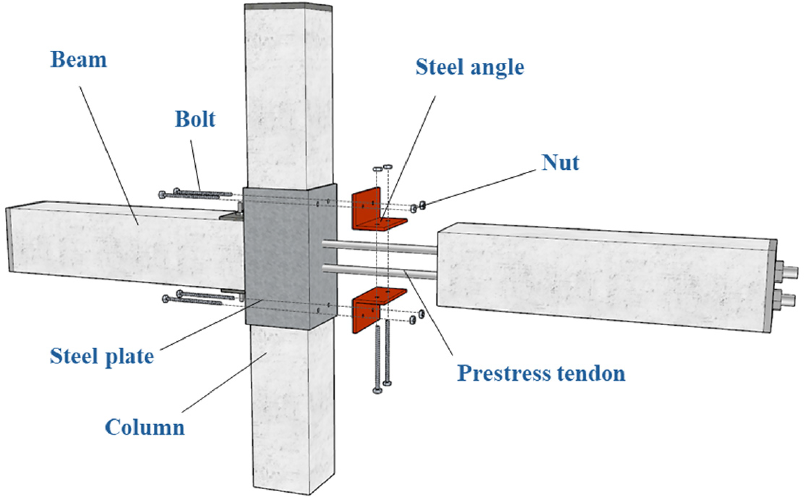
Schematic of an SC joint. SC: self-centering.

Figure 2.

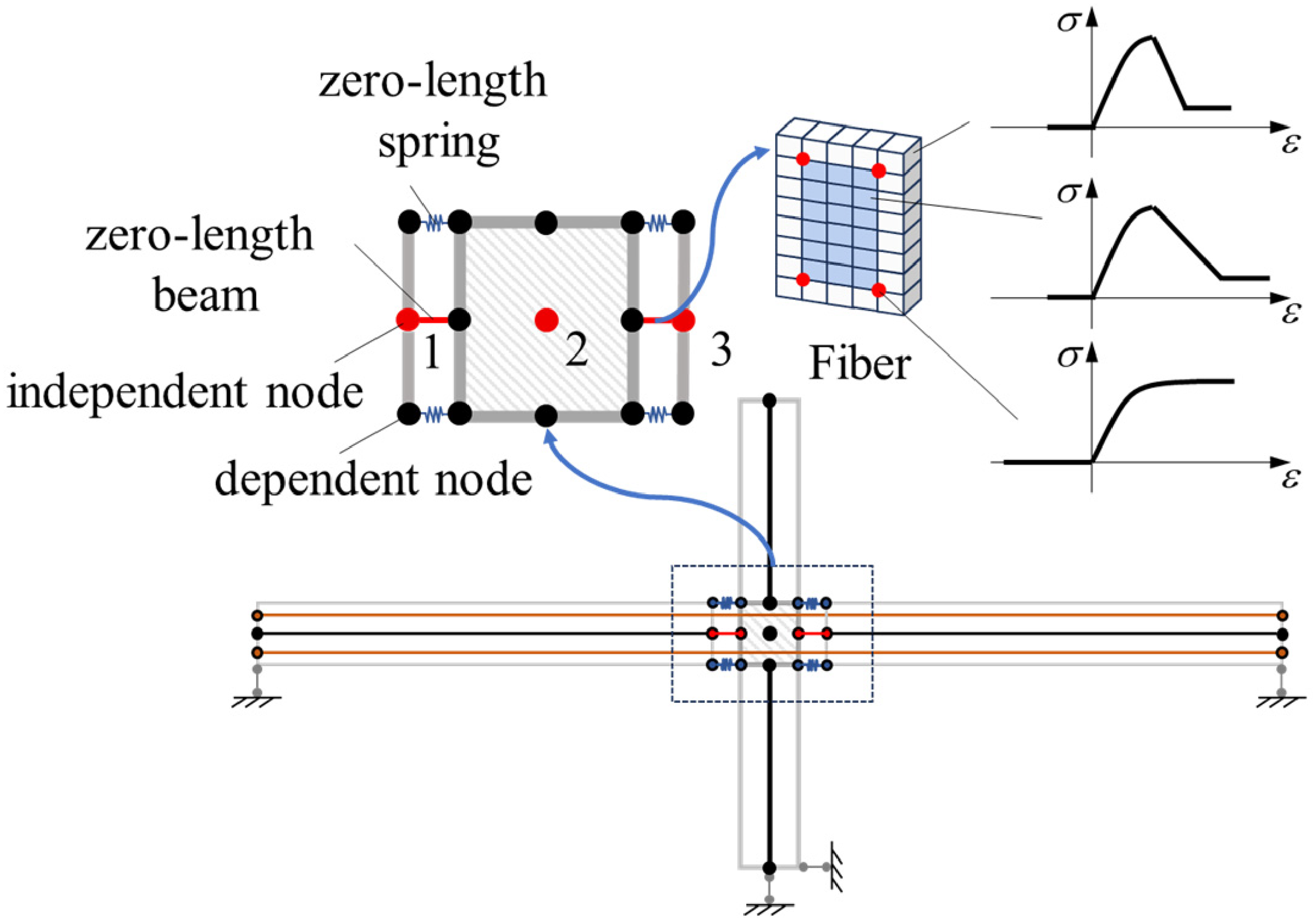
Components of a VL element. VL: VFIFE-link; VFIFE: vector form intrinsic finite element.

The VL element consists of 15 nodes, including three independent nodes (nodes 1, 2, and 3) and 12 dependent nodes (nodes 4–15). As illustrated in Figure 3, the center of the VL element is modeled as a rigid plate governed by the motion of independent node 2, while the dependent nodes on its edges are kinematically linked through rigid-body constraints defined by the rotation $θ_{2}$ and geometric offsets $(h / 2, b / 2)$ . Similarly, the angle steel nodes on the beam side are connected to their corresponding independent nodes (1 and 3) via rigid arms. In this model, the angle steel is represented by zero-length springs, while the beam–column interaction is simulated by a zero-length element discretized into multiple fibers, each assigned a specific constitutive model that neglects tensile strength. Within the unified VFIFE framework, the opening and closing states of the joints are accurately determined by monitoring the geometric distance $δ$ between opposing dependent nodes:

δ = (x_{p} - x_{m}) \cdot n_{m n} - R \leq 0

(1)

where

x_{p}

and

x_{m}

are the displacement vectors of nodes m and n, respectively;

n_{m n}

is the normal vector of mn; and R is a small number that is infinitely close to zero.

Figure 3.

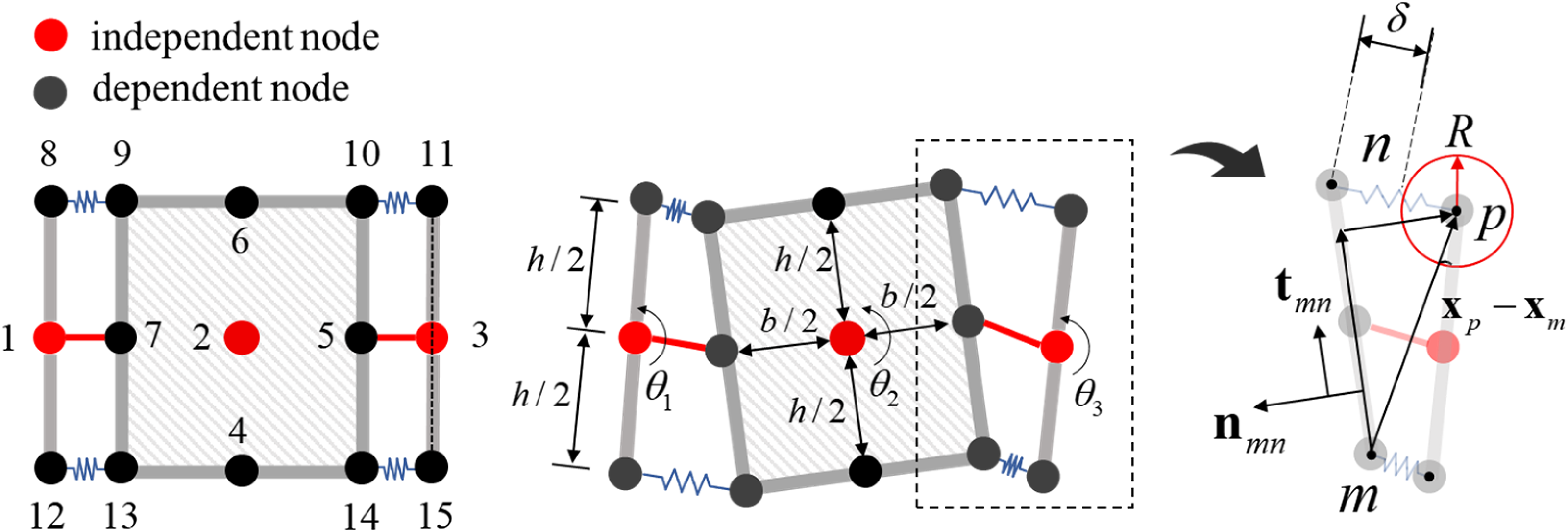
Schematic diagram of the VL element with labeled nodes and kinematic relationship. VL: VFIFE-link; VFIFE: vector form intrinsic finite element.

When $δ > 0$ , the gap is open and the compressive zero-length spring forces are deactivated; when $δ \leq 0$ , contact is detected, and compressive forces are activated to simulate the contact–impact dynamics and prevent interpenetration.

Internal-force integration of VL element

The following describes the integration of forces in a VL element. As described in the section “Proposed VL element,” the gray rectangle area represents a rigid plate that only undergoes rigid-body translation and rotation without deformation. For clarity, a force diagram is provided, as shown in Figure 4.

Figure 4.

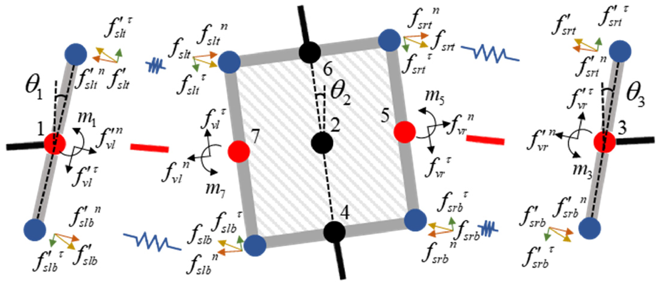
Diagram of force integration.

The resultant forces between the beam and column consist of internal forces from two beams and four springs. The forces on the left are denoted by the subscript l, while those on the right are denoted by the subscript r. Since the calculation procedures for both sides are identical, only the left side is used for illustration.

The force on node 7 is decomposed into the tangential component $f_{v l}^{τ}$ , normal component $f_{v l}^{n}$ , and moment $m_{7}$ . The forces on node 1 are denoted by $f_{v l}^{' τ}$ , $f_{v l}^{' n}$ , and $m_{1}$ (all equal in magnitude to those on node 7 but in the opposite direction). These forces are obtained in equation (2) as follows:

F = {\begin{matrix} | f_{v l}^{n} | \\ | f_{v l}^{τ} | \\ m_{1} \\ m_{7} \end{matrix}} = {\begin{matrix} \int_{0}^{l} d s \int \int σ d_{A} \\ \int_{0}^{l} (4 - 6 s) d s \int \int σ y d_{A} + \int_{0}^{l} (2 - 6 s) d s \int \int σ y d_{A} \\ \int_{0}^{l} (4 - 6 s) d s \int \int σ y d_{A} \\ \int_{0}^{l} (2 - 6 s) d s \int \int σ y d_{A} \end{matrix}}

(2)

where

s = x / l

; l represents the length of the beam and A represents the area of the beam.

As shown in Figure 4, the coordinates of nodes 4, 5, 6, and 7 are obtained using equations (3), (4), (5), and (6) as follows:

(x_{4}, y_{4}) = (x_{2} + \frac{h}{2} \sin (θ_{2}), y_{2} - \frac{h}{2} \cos (θ_{2}))

(3)

(x_{5}, y_{5}) = (x_{2} + \frac{b}{2} \cos (θ_{2}), y_{2} + \frac{b}{2} \sin (θ_{2}))

(4)

(x_{6}, y_{6}) = (x_{2} - \frac{h}{2} \sin (θ_{2}), y_{2} + \frac{h}{2} \cos (θ_{2}))

(5)

(x_{7}, y_{7}) = (x_{2} - \frac{b}{2} \cos (θ_{2}), y_{2} - \frac{b}{2} \sin (θ_{2}))

(6)

where

θ_{2}

represents the rotation angle of node 2; b represents the width of the column; h represents the height of the beam; and x, y are the coordinates of the nodes.

The left-top angle steel is denoted by subscript $s l t$ and the left-bottom angle steel is denoted by subscript $s l b$ ; similarly, subscripts $s r t$ and $s r b$ are used to indicate right-top and right-bottom angle steels, respectively. The location of the two angle steels on the left can then be obtained by equations (6) to (9), using the locations of nodes 1 and 7 as follows:

(x_{s l t}, y_{s l t}) = (x_{7} + \frac{h}{2} \sin (θ_{2}), y_{7} + \frac{h}{2} \cos (θ_{2}))

(7)

(x_{s l b}, y_{s l b}) = (x_{7} - \frac{h}{2} \sin (θ_{2}), y_{7} - \frac{h}{2} \cos (θ_{2}))

(8)

({x^{'}}_{s l t}, {y^{'}}_{s l t}) = (x_{1} + \frac{h}{2} \sin (θ_{1}), y_{1} + \frac{h}{2} \cos (θ_{1}))

(9)

({x^{'}}_{s l b}, {y^{'}}_{s l b}) = (x_{1} - \frac{h}{2} \sin (θ_{1}), y_{1} - \frac{h}{2} \cos (θ_{1}))

(10)

where

θ_{1}

represents the rotation angle of node 1.

Additionally, the internal forces of the zero-length spring are decomposed into tangential and normal components. Considering the left-top angle steel as an example, the corresponding normal and tangential forces can be obtained by equations (11), (12), (13), and (14) as follows:

f_{s l t}^{n} = f_{s l t} \frac{(x_{s l t} - {x^{'}}_{s l t}) (x_{5} - x_{7}) + (y_{s l t} - {y^{'}}_{s l t}) (y_{5} - y_{7})}{\sqrt{{(x_{s l t} - {x^{'}}_{s l t})}^{2} + {(y_{s l t} - {y^{'}}_{s l t})}^{2}} \sqrt{{(x_{5} - x_{7})}^{2} + {(y_{5} - y_{7})}^{2}}}

(11)

f_{s l t}^{τ} = f_{s l t} \sqrt{1 - {(\frac{(x_{s l t} - {x^{'}}_{s l t}) (x_{5} - x_{7}) + (y_{s l t} - {y^{'}}_{s l t}) (y_{5} - y_{7})}{\sqrt{{(x_{s l t} - {x^{'}}_{s l t})}^{2} + {(y_{s l t} - {y^{'}}_{s l t})}^{2}} \sqrt{{(x_{5} - x_{7})}^{2} + {(y_{5} - y_{7})}^{2}}})}^{2}}

(12)

f_{s l t}^{' n} = f_{s l t}^{'} \sqrt{1 - {(\frac{(x_{s l t} - {x^{'}}_{s l t}) (x_{s l b} - x_{s l t}) + (y_{s l t} - {y^{'}}_{s l t}) (y_{s l b} - y_{s l t})}{\sqrt{{(x_{s l t} - {x^{'}}_{s l t})}^{2} + {(y_{s l t} - {y^{'}}_{s l t})}^{2}} \sqrt{{(x_{s l b} - x_{s l t})}^{2} + {(y_{s l b} - y_{s l t})}^{2}}})}^{2}}

(13)

f_{s l t}^{' τ} = f_{s l t}^{'} \frac{(x_{s l t} - {x^{'}}_{s l t}) (x_{s l b} - x_{s l t}) + (y_{s l t} - {y^{'}}_{s l t}) (y_{s l b} - y_{s l t})}{\sqrt{{(x_{s l t} - {x^{'}}_{s l t})}^{2} + {(y_{s l t} - {y^{'}}_{s l t})}^{2}} \sqrt{{(x_{s l b} - x_{s l t})}^{2} + {(y_{s l b} - y_{s l t})}^{2}}}

(14)

where

f_{s l t}^{n}

represents the normal internal forces on the rigid area and

f_{s l t}^{τ}

represents the tangential internal forces on the rigid area.

f_{s l t}^{' n}

f_{s l t}^{' τ}

represent the reaction forces on the beam. The internal forces for the other angle steels can be obtained by following the same steps.

The internal force of each component needs to be integrated into the independent nodes (nodes 1, 2, and 3). The resultant force on node 1 can be obtained by equation (15). The resultant force on node 3 follows the same steps as node 1, while the force on node 2 is obtained using equation (16) as follows:

{\begin{matrix} f_{1}^{τ} = {f^{'}}_{s l t}^{τ} - {f^{'}}_{v l}^{τ} - {f^{'}}_{s l b}^{τ} \\ f_{1}^{n} = - {f^{'}}_{s l t}^{n} + {f^{'}}_{v l}^{n} + {f^{'}}_{s l b}^{n} \\ M_{1} = m_{1} + \frac{h}{2} ({f^{'}}_{s l t}^{n} + {f^{'}}_{s l b}^{n}) \end{matrix}

(15)

{\begin{matrix} f_{2}^{τ} = - f_{s l t}^{τ} + f_{v l}^{τ} + f_{s l b}^{τ} - f_{s r t}^{τ} - f_{v r}^{τ} + f_{s r b}^{τ} \\ f_{2}^{n} = f_{s l t}^{n} - f_{v l}^{n} - f_{s l b}^{n} + f_{s r t}^{n} + f_{v r}^{n} - f_{s r b}^{n} \\ M_{2} = m_{7} + m_{5} - \frac{h}{2} (f_{s l t}^{n} + f_{s l b}^{n} + f_{s r t}^{n} + f_{s r b}^{n}) \end{matrix}

(16)

Note that a rotation matrix is required to transform all the forces into the global coordinate system.

VFIFE simulation

Basics of VFIFE method

Point value description

As shown in Figure 5, the structure is discretized into finite mass particles and massless elements. The motion of the mass particles follows Newton's second law:

m x^{″} = F^{e x t} + F^{i n t}

(17)

where m represents the mass of the particle;

x^{″}

represents the acceleration of the particle;

F^{e x t}

represents the external force; and

F^{i n t}

represents the internal force.

Figure 5.

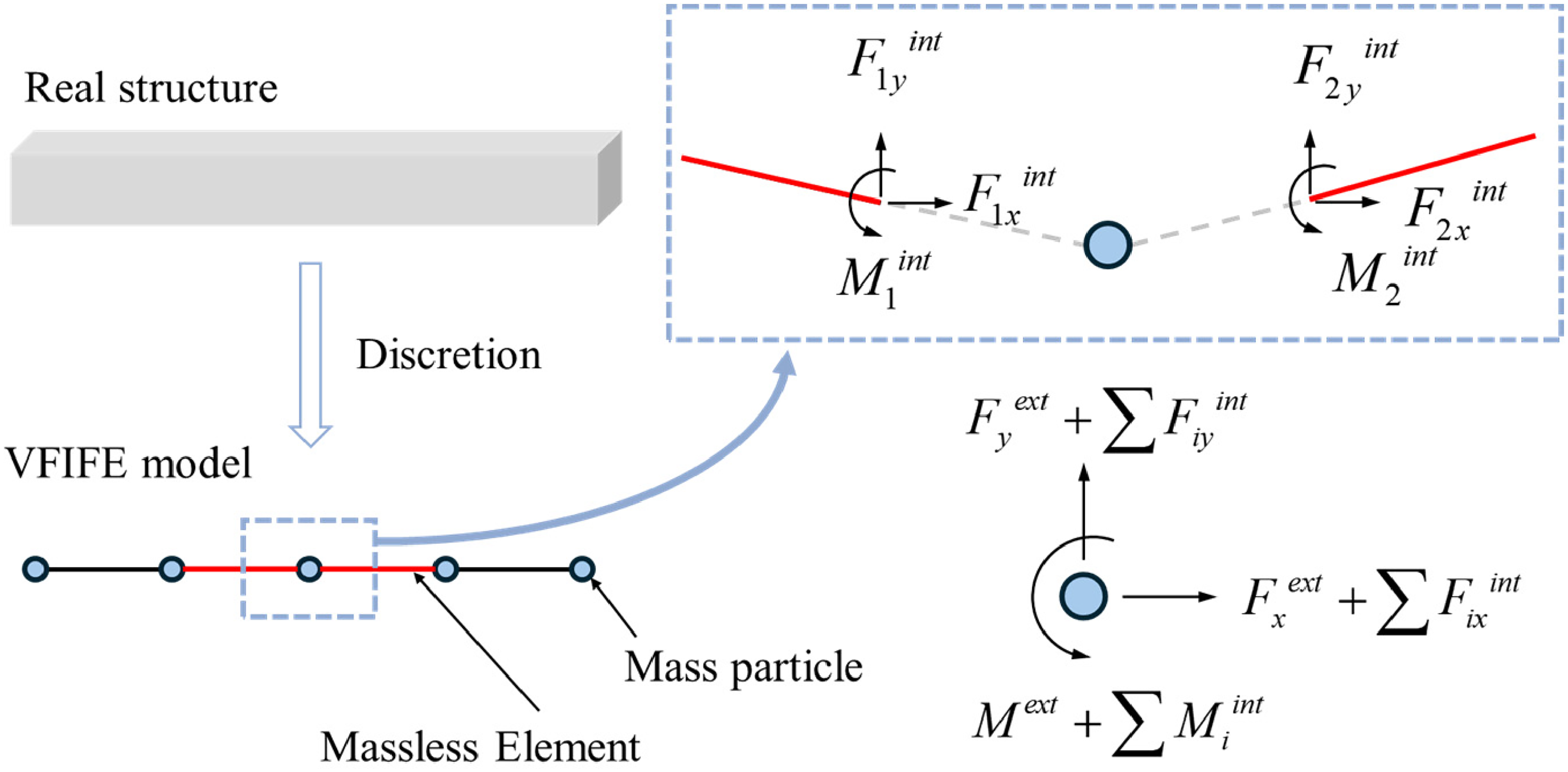
Point value description.

The central difference method is used to solve the equations of motion, as described in equations (17) to (20). It should be noted that equation (18) is adopted for the initial step, while equation (19) is used for non-initial steps, as follows:

x_{J, 1} = x_{J, 2} - \frac{h}{C_{1}} {x^{'}}_{J, 2} + \frac{1}{2} h^{2} m_{J}^{- 1} F_{J, 2}

(18)

x_{J, i + 1} = C_{1} m_{J}^{- 1} F_{J, i} h^{2} + 2 C_{1} x_{J, i} - C_{2} x_{J, i - 1}

(19)

C_{1} = {(1 + \frac{ζ h}{2})}^{- 1}, C_{2} = C_{1} (1 - \frac{ζ h}{2})

(20)

F_{J, i} = E_{J, i} + I_{J, i}, m_{J} = diag (m_{J x}, m_{J y}, I_{J z})

(21)

where

m_{J}

represents the mass matrix of the j-th particle;

E_{J, i}

represents the external force on the j-th particle at i-th time step;

I_{J, i}

represents the internal load on the j-th particle at i-th time step; and

ζ

represents the damping factor.

Path element

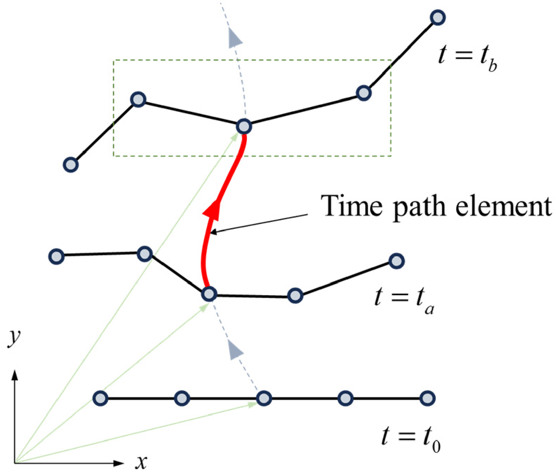
In the time domain, the structural motion is discretized into a series of path elements, as shown in Figure 6. Within a path element $t \in [t_{a}, t_{b}]$ , the motions of the mass particles are considered continuous, and the elements undergo small deformations but possibly large displacements, allowing for large rigid-body movement. Between two continuous path elements, the motions of the mass particles, structural configuration, forcing condition, and mechanical characteristics of the elements can all be discontinuous. This characteristic makes VFIFE a powerful tool for solving the large deformation, contact, and fracture problems.

Figure 6.

Time path element.

Fictitious reverse motion

To decouple rigid-body motion from pure deformation, a fictitious reverse motion is introduced, as shown in Figure 7. Within a path element $[t_{a}, t_{b}]$ , suppose the configuration of an element is $1^{'} - 2^{'}$ . First, translate the element by $- Δ d_{1}$ , so that $1^{'}$ and $1^{a}$ are aligned at the same position. Subsequently, rotate the element by $- Δ θ$ around $1^{a}$ . The value of $Δ θ$ can be estimated as follows:

Δ θ = \cos^{- 1} (e^{a} \cdot e^{'})

(22)

where

e^{a}

represents the direction vector at

t_{a}

and

e^{'}

represents the direction vector at

t^{'}

Figure 7.

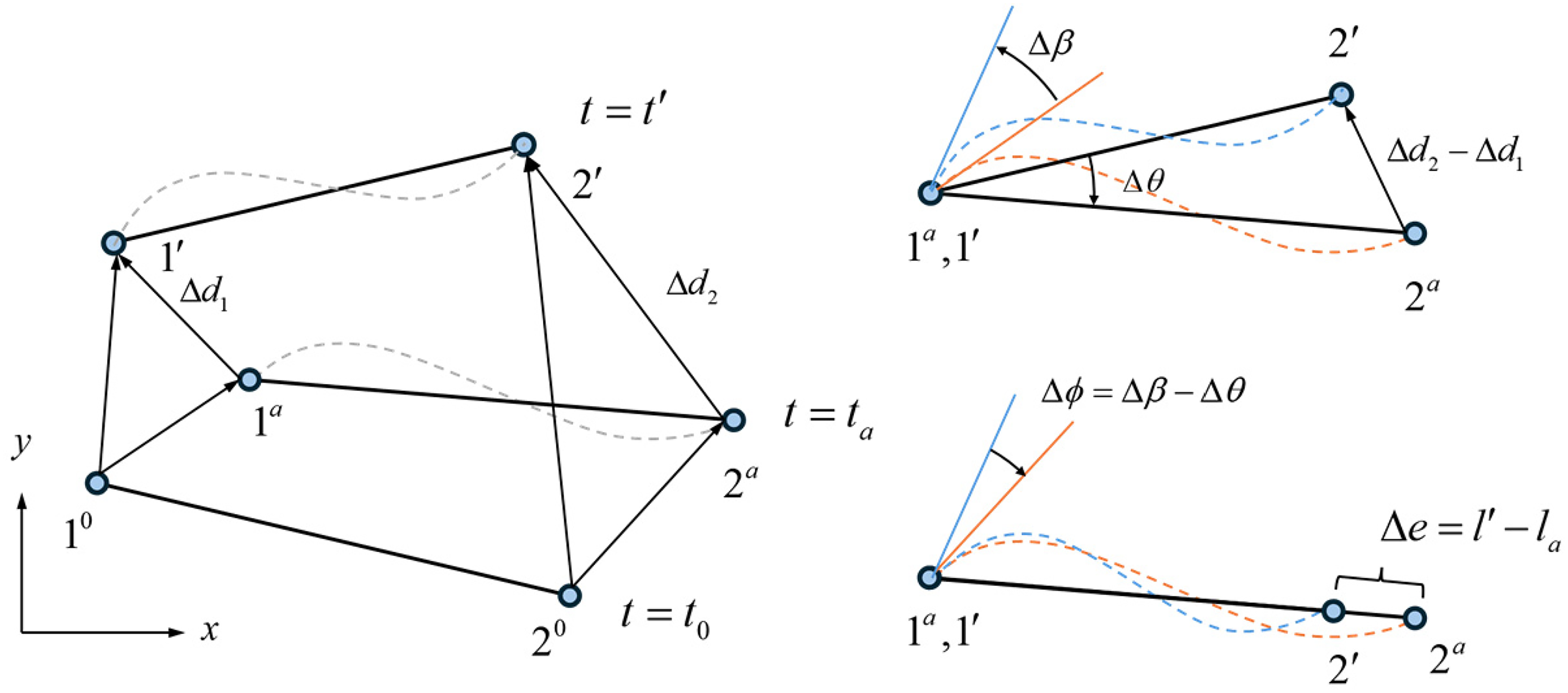
Fictitious reverse motion.

The pure deformation $Δ \hat{u}$ for a planar beam element can be obtained as follows:

Δ \hat{u} = [{\begin{matrix} Δ e & Δ ϕ_{1} & Δ ϕ \end{matrix}}_{2}]^{T}

(23)

where

Δ e = l^{'} - l_{a}

;

Δ ϕ_{1} = Δ β_{1} - Δ θ

; and

Δ ϕ_{2} = Δ β_{2} - Δ θ

VFIFE model of SC joint

When performing VFIFE simulations, the basic computational assumptions are adopted: (a) the deformation of beams and columns follows the plane section assumption; (b) no slippage occurs between the angle steel and beam–column; (c) bond-slip effects between concrete and steel bars are negligible; and (d) friction between the pre-stressed tendons and embedded polyvinyl chloride pipes is neglected. Detailed models of the T-shaped and cross-shaped SC joints are shown in Figure 8(a) and (b), respectively.

Figure 8.

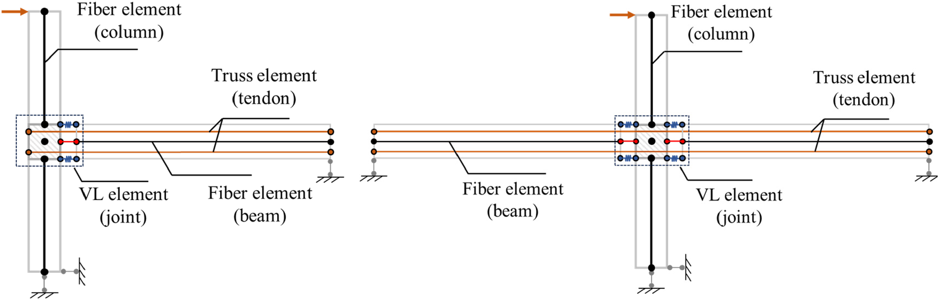
VFIFE model: (a) T-shaped joint and (b) cross-shaped joint. VFIFE: vector form intrinsic finite element.

The dependent nodes in the VL element are treated as zero-mass nodes, capable of transferring forces to the remaining parts of the joint. Beams and columns are modeled using fiber elements with 20 fiber layers, while pre-stressed tendons are represented by cable elements. In the T-shaped joint, the tendons are anchored between the left side of the column and the right side of the beam, as shown in Figure 8(a). In the cross-shaped joint, the tendons are anchored between the left and right edges of the beam, as shown in Figure 8(b). The pre-stressing force is introduced by applying an initial stress to the cable elements.

The aforementioned model was completely developed based on the actual working conditions of the structure, with each element having a clear physical meaning and corresponding parameters. Since the VFIFE method employs point-value descriptions and is not constrained by the assumptions of small and continuous deformation, the behavior of nodes, including their opening and closing, can be accurately represented through the calculated node states throughout the simulation process. This provides an effective method for understanding the node opening and closing process.

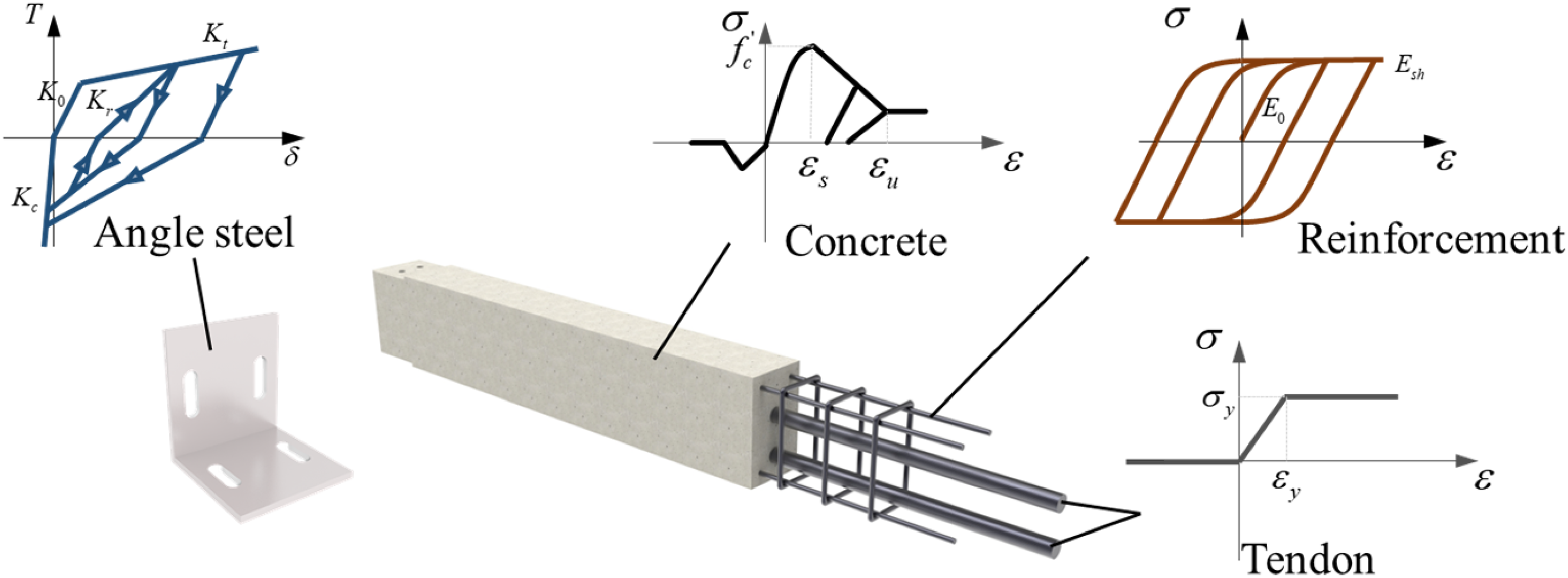
As illustrated in Figure 9, the confined concrete constitutive model is applied to the beams and columns in the core region (Kent and Park, 1971), while the concrete in the non-core region is modeled using the unconfined concrete constitutive model (Scott et al., 1982). The Menegotto–Pinto model is employed in the longitudinal reinforcements (Menegotto, 1973), while a bilinear model is applied to the pre-stressed tendons without compression strength (Resapu and Perumahanthi, 2021). The model proposed by Garlock et al. was used to simulate angle steel (Garlock et al., 2003).

Figure 9.

Constitutive models for each part of the SC joint. SC: self-centering.

The Kent and Park model was selected because it effectively captures the strength enhancement and ductility provided by the transverse confinement, which is crucial for the core concrete subjected to severe localized compressive stresses during joint gap closure. Furthermore, the Menegotto–Pinto model is utilized for the reinforcement as it accurately reflects the Bauschinger effect under cyclic loading, a characteristic that directly contributes to the hysteretic energy dissipation and the characteristic pinching effect observed in the structural response of SC joints.

The constitutive model parameters utilized in the simulation, including the concrete, reinforcements, angle steel, and the tendons, were calibrated based on standard uniaxial tests conducted prior to the joint testing. The relevant material properties are listed in Table 1.

Table 1.

Material properties.

Type	Yield strength (MPa)	Ultimate strength (MPa)	Elastic modulus (MPa)
Concrete	–	88	4.2 × 10⁴
Reinforcement	495	585	2.0 × 10⁵
Tendon	1640	1860	1.95 × 10⁵
Angle steel	270	400	2.0 × 10⁵

Calculation process of the structural response

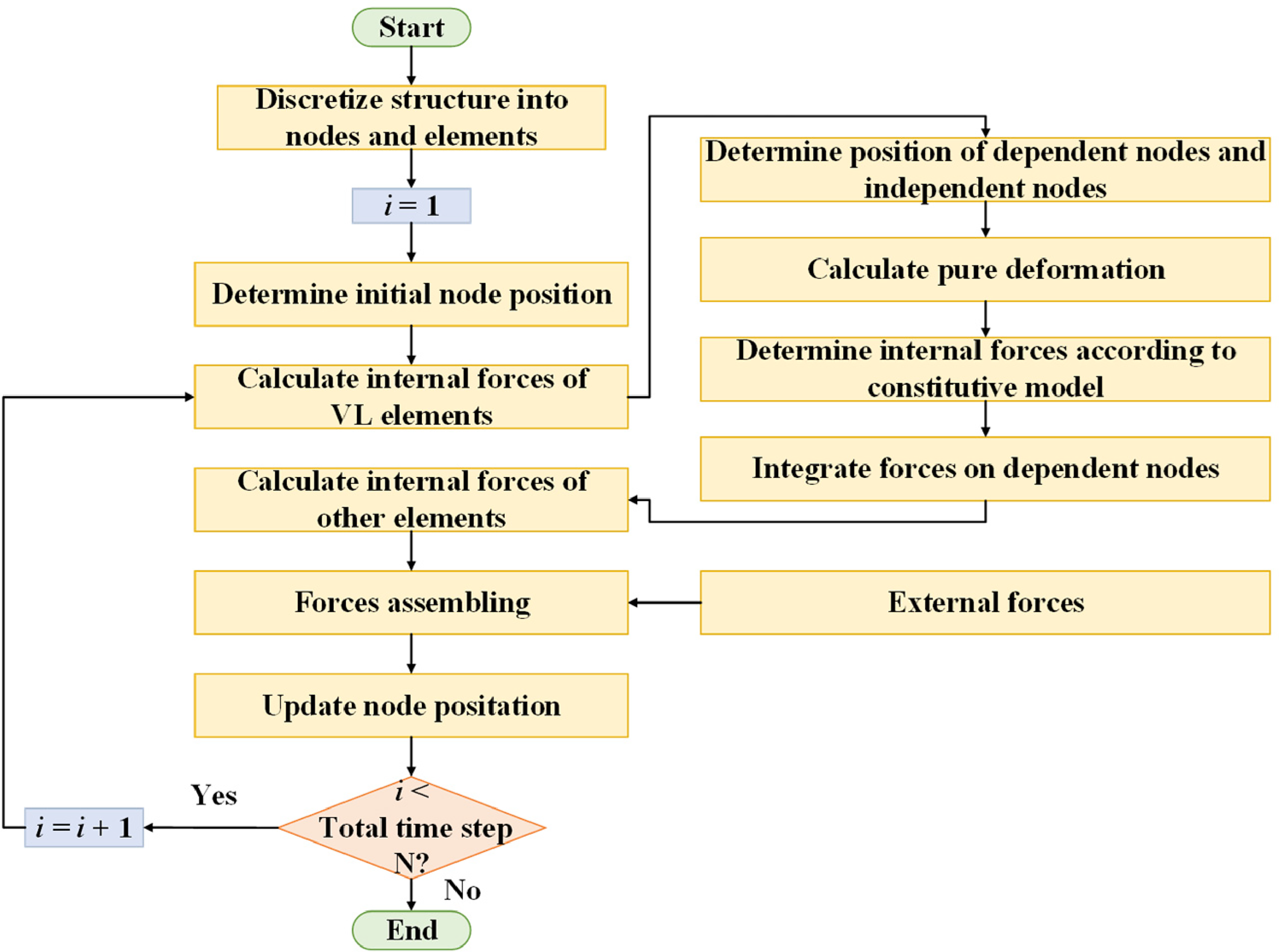
The entire VFIFE calculation process is shown in Figure 10, where i represents the i-th time step, and N represents the total number of steps. The procedure begins with the discretization of the structure into nodes and elements, and the initial node positions are determined using the physical dimensions. Subsequently, an iterative calculation is performed for each time step i. This process starts with the calculation of internal forces, which is central to the workflow. It prioritizes the proposed VL elements by determining the positions of independent and dependent nodes, calculating pure deformation, deriving internal forces from the constitutive model, and integrating these forces on the dependent nodes before calculating the forces for other element types. Subsequently, all internal forces are combined with external loads to determine the resultant force on each node. Finally, the central difference method is employed to update each node's position based on the resultant force, resulting in the new structural configuration. This iterative process continues from i = 1 until all time steps have been completed (i > N), ultimately providing the full dynamic response of the structure under excitation.

Figure 10.

Flowchart of VFIFE calculation process. VFIFE: vector form intrinsic finite element.

Experimental validation

Design of SC joint

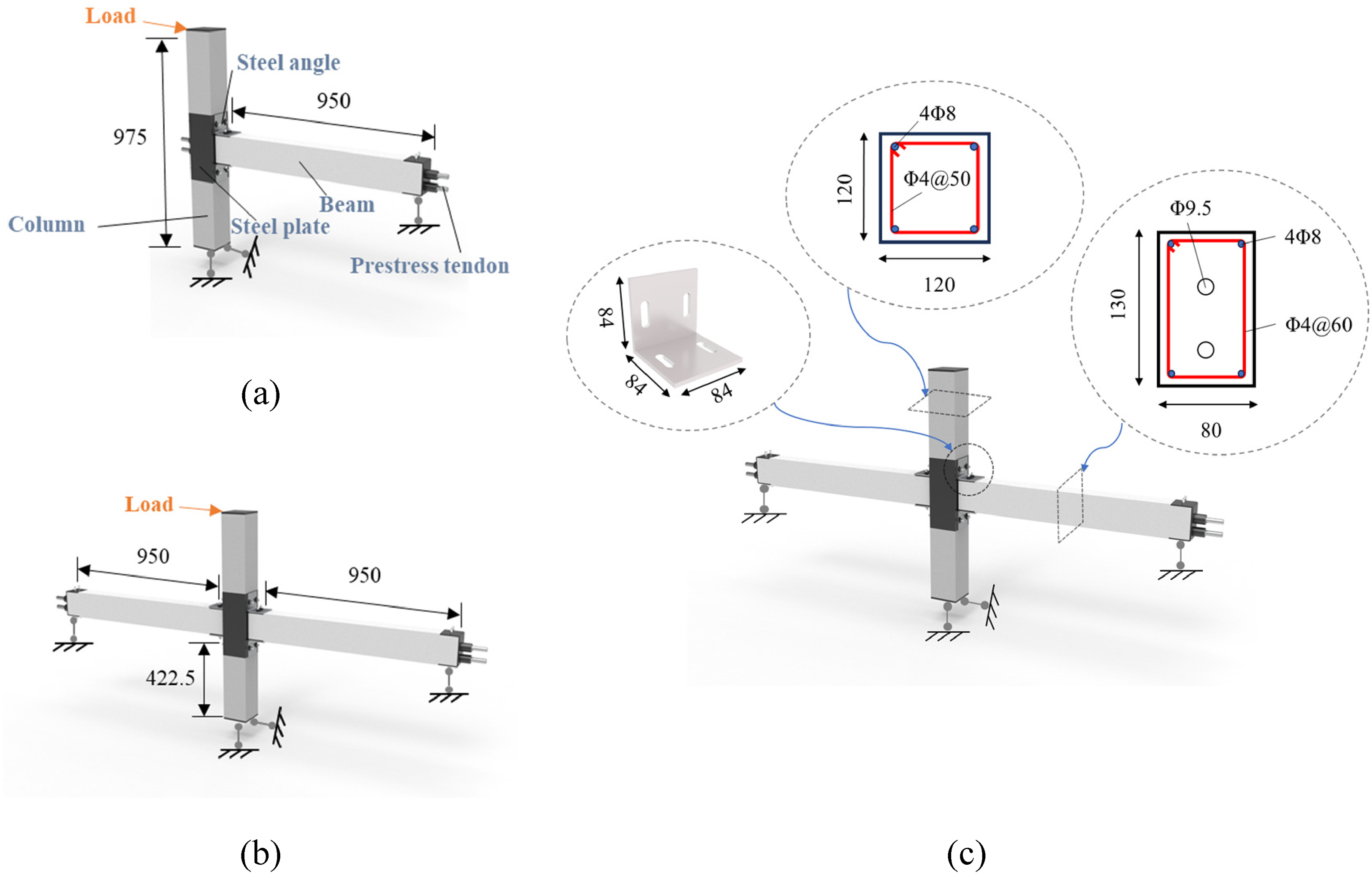
Two types of SC joints, namely T-shaped and cross-shaped joints, are designed and fabricated to validate the proposed simulation method. The structural configurations are shown in Figure 11. To prevent concrete crushing during the loading process, steel plates are embedded at both the loading point and the fixed end.

Figure 11.

Test specimens: (a) T-shaped joint, (b) cross-shaped joint, and (c) sectional properties (unit: mm).

Loading device and instrumentation

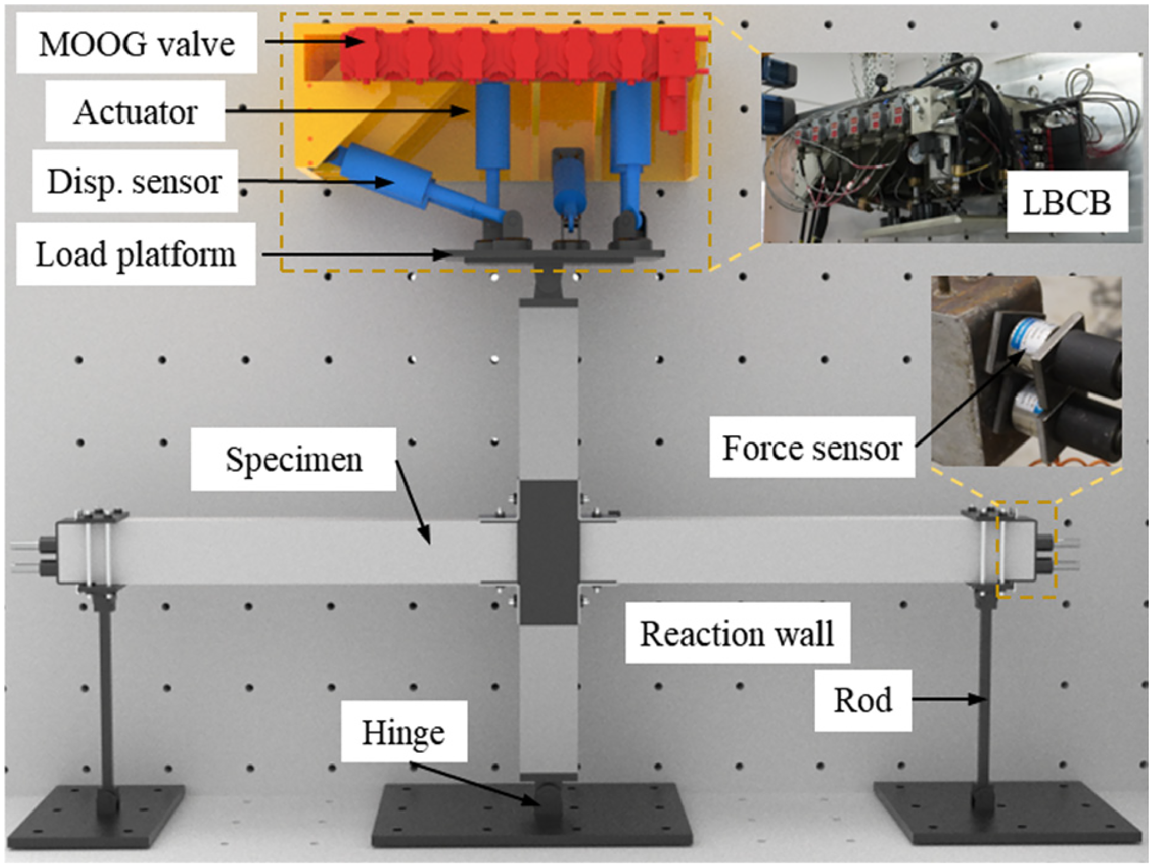
The pseudo-dynamic tests are conducted at Zhejiang University. Displacement-controlled loading is performed using a load and boundary condition box (LBCB). An LBCB consists of six hydraulic actuators, each of which is equipped with displacement and force sensors. They work together to ensure that the connected loading platform follows the prescribed loading curve during the test. The schematic test setup of the cross-shaped joint is illustrated in Figure 12. Pre-fabricated hinge supports, chain rods, and steel plates were used to secure the specimen to the reaction wall and reaction floor. The top of the specimen is connected to the LBCB.

Figure 12.

Schematic of pseudo-dynamic tests.

Prior to testing, the tendons were pre-stressed to 20% of their ultimate strength. Two force sensors were installed to measure changes in internal forces and were fixed to the ends of the tendons using anchors, as shown in Figure 12.

Loading sequence

The loading sequence was derived from the response record of a shaking table test conducted on an SC frame structure with the same joint configuration (Zhang, Fang et al., 2025), based on the top floor displacement response under two simulated seismic excitations: (1) the Chi-Chi pulse-type seismic wave and (2) a synthetic artificial seismic wave.

The loading device enables precise application of complex time history loads and boundary conditions. Thus, four loading curves named L1–L4 in Figure 13 are used in the pseudo-dynamic test. The displacement time histories (L1–L4) were extracted directly from the displacement sensors installed on the top floor of the frame during the shake table test and converted into the target lateral drift inputs for the LBCB actuators. Displacement-controlled loading is applied in this pseudo-dynamic test, with rightward displacement defined as positive. For convenience, the cases for T-shaped joints are labeled TL1–TL4, while those for cross-shaped joints are labeled CL1–CL4.

Figure 13.

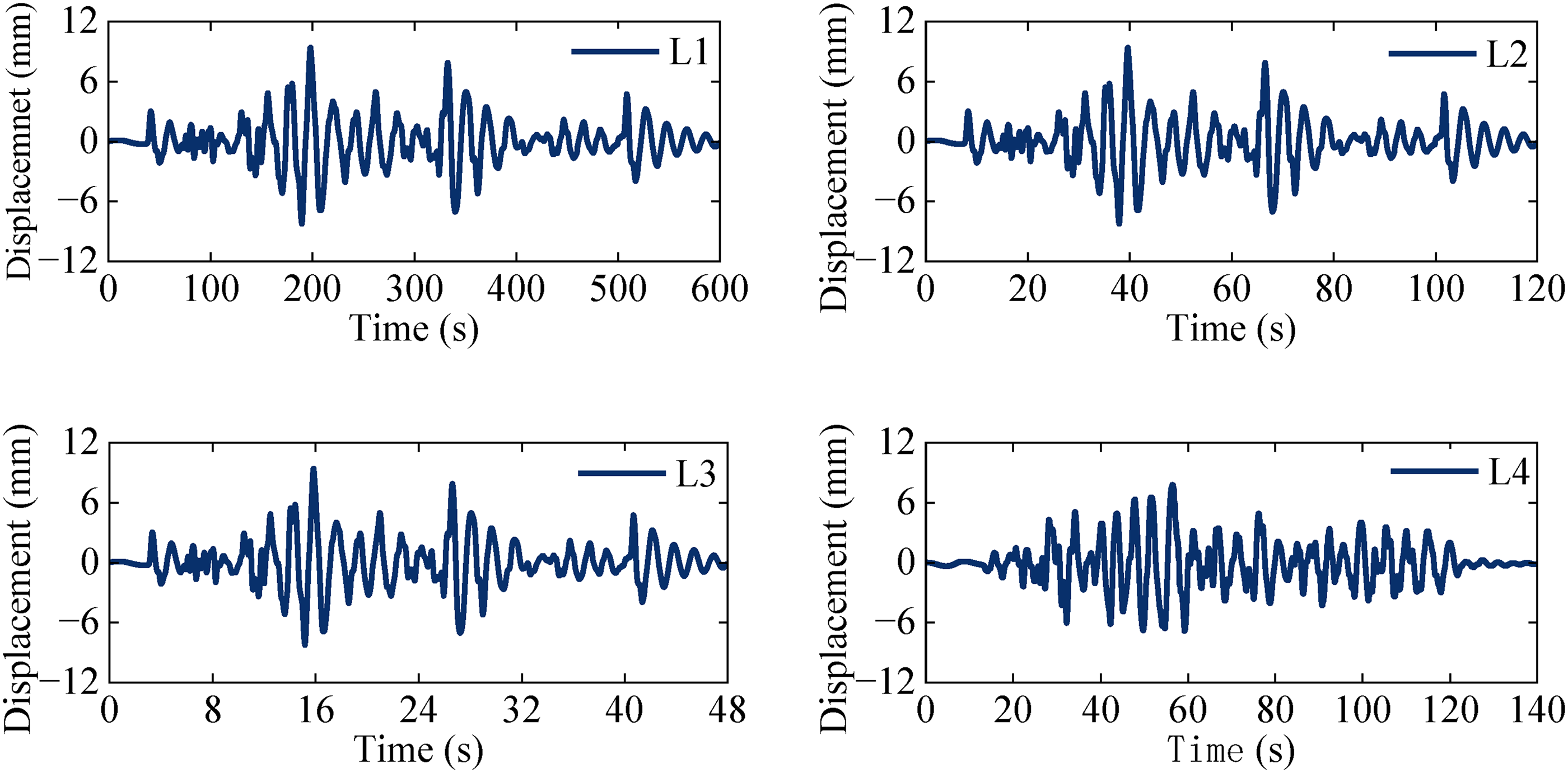
Loading curves for the pseudo-dynamic tests.

Simulation results and comparison

Three kinds of responses: (a) hysteresis curves; (b) gap opening rotation; and (c) pre-stressing force change in the tendons were compared and analyzed.

Hysteresis curves

The comparison results of hysteresis curves are shown in Figure 14. The simulation results from the VFIFE model (dashed line) are in good agreement with the experimental data (solid line) in terms of curve shape and stiffness degradation trends. In this simulation, the maximum drift ratio was approximately 1.03%. This level of drift is near the collapse prevention limit for structures under rare earthquake events. Even with such large deformations, the VFIFE model accurately simulates the displacement response. This demonstrates the model's high-fidelity predictive capability, even when the structure approaches the maximum collapse prevention state specified by design codes.

Figure 14.

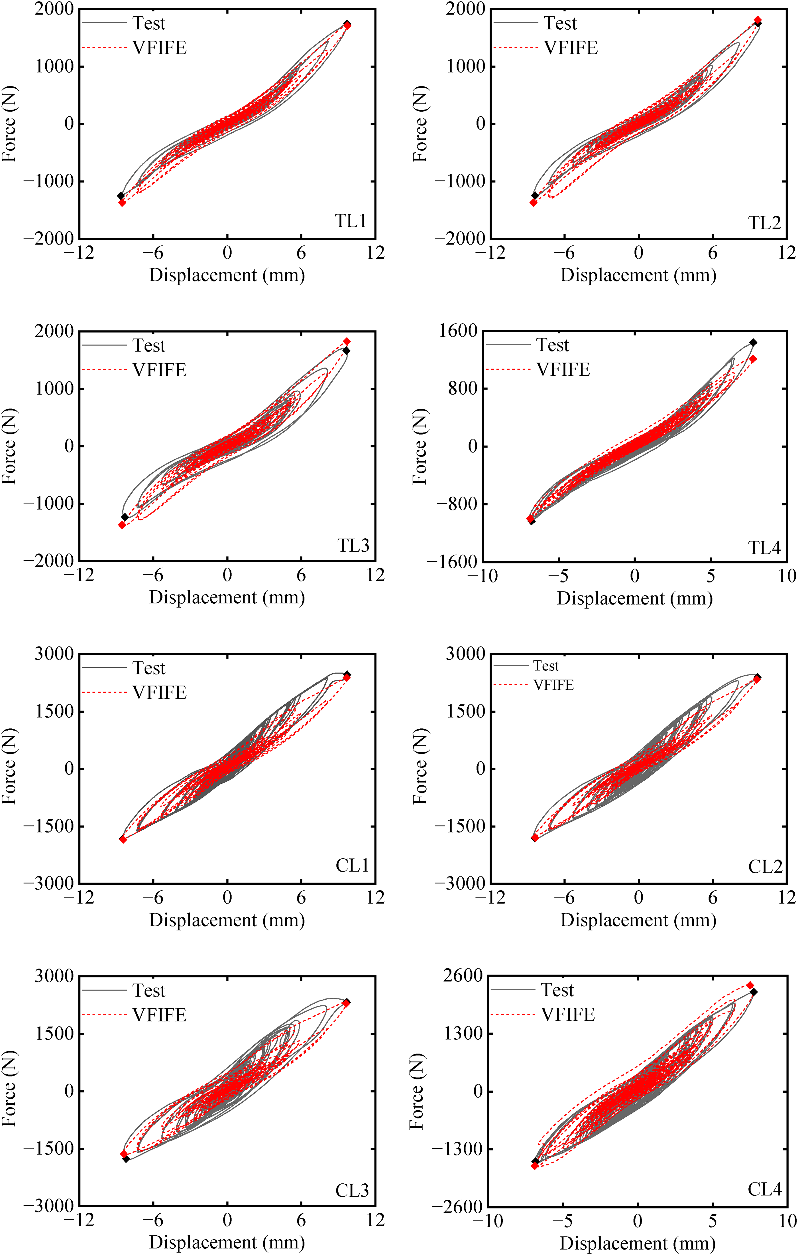
Comparison results of hysteretic curves.

The coefficient of determination R² and normalized root mean square error (NRMSE) were used to assess the accuracy of the VFIFE method. The R² and NRMSE for hysteretic curves are listed in Table 2. For the T-shaped joints (TL1–TL4), the consistently high R² values (95.30–97.32%) indicate that the VFIFE model captures over 95% of the variance in the experimental data, demonstrating excellent agreement with real behavior. The low NRMSE values (2.84–4.96%) further confirm that the prediction errors remain minimal, thereby reinforcing the model's precision in simulating T-shaped joint responses. In contrast, the cross-shaped joints (CL1–CL4) exhibit slightly lower R² values (92.22–95.64%) and higher NRMSE values (5.41–6.85%), indicating that the VFIFE model experiences greater difficulty in fully capturing their mechanical behavior. This difference can be attributed to the increased complexity of their experimental boundary constraints compared to T-shaped configurations. While the numerical model assumes idealized pin supports at the beam ends, the actual experimental hinges involve bearings with internal clearances (gaps) and frictional resistance. In cross-shaped joints, which involve more support points and a more symmetric but constrained setup. Furthermore, the current modeling approach neglects the friction between the pre-stressed tendons and the internal ducts within the beam–column core. Given that tendons in cross-shaped joints typically traverse a more complex interaction zone with potentially higher stress gradients.

Table 2.

Coefficient of determination and NRMSE of hysteresis curves.

Joint type	Case	R² (%)	NRMSE (%)
T-shaped	TL1	97.32	2.84
	TL2	97.01	2.73
	TL3	95.87	3.03
	TL4	95.30	4.96
Cross-shaped	CL1	95.64	5.41
	CL2	95.13	5.74
	CL3	94.54	6.61
	CL4	92.22	6.85

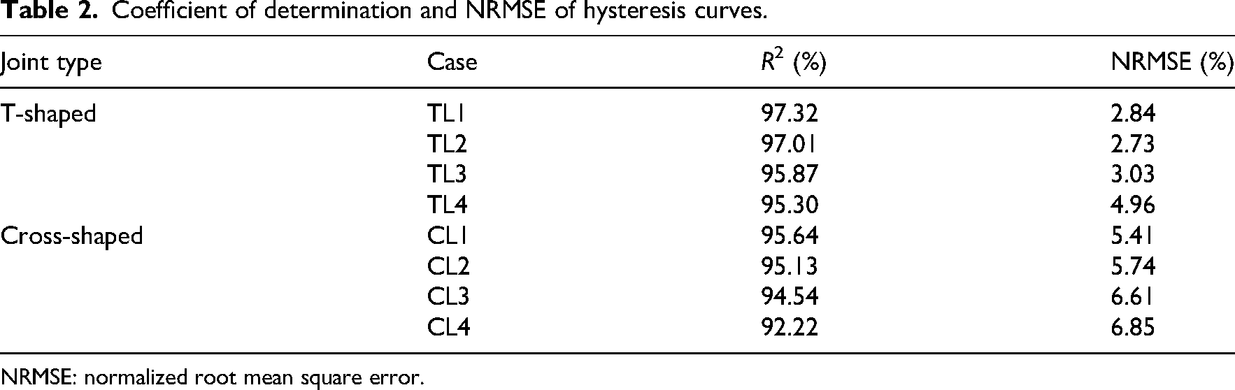
NRMSE: normalized root mean square error.

Gap rotation

The simulation of gap rotation is essential for accurately capturing the cyclic opening and closing behavior of the SC joint under seismic loading. As shown in Figure 15, the gap rotation is obtained using two vectors defined by nodes on the angle steel. The rotation is calculated by the following equation:

θ = \cos^{- 1} \frac{v e c \cdot v e c^{'}}{| v e c | | v e c^{'} |}

(24)

Figure 15.

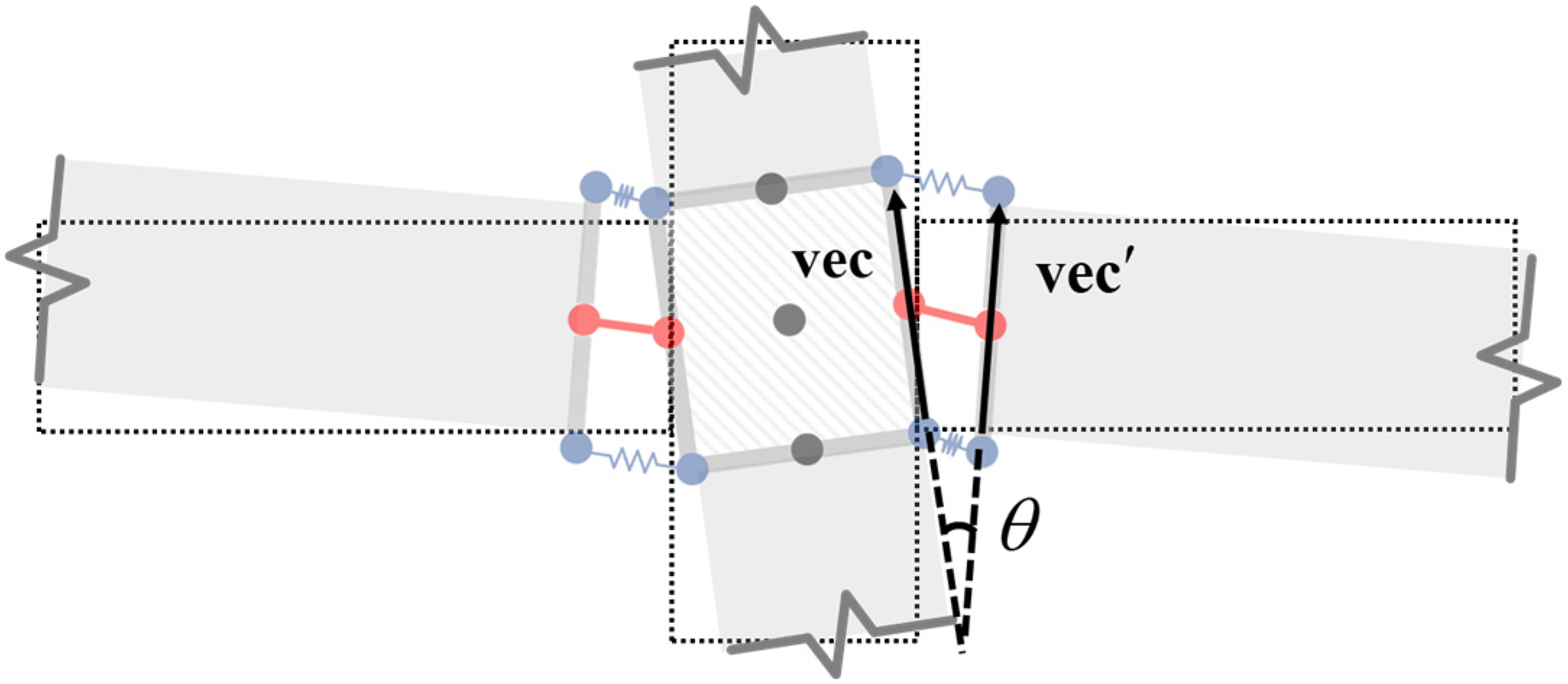
Calculation diagram of gap rotation.

Figure 16 presents the time history results for gap rotation. In each plot, the simulated response from the VFIFE model (dashed line) is compared with the corresponding experimental test data (solid line) for the eight loading cases (TL1–TL4 and CL1–CL4). A qualitative inspection indicated that the model effectively captures the overall pattern and timing of the gap rotation throughout the seismic events, providing a basis for the detailed quantitative analysis that follows.

Figure 16.

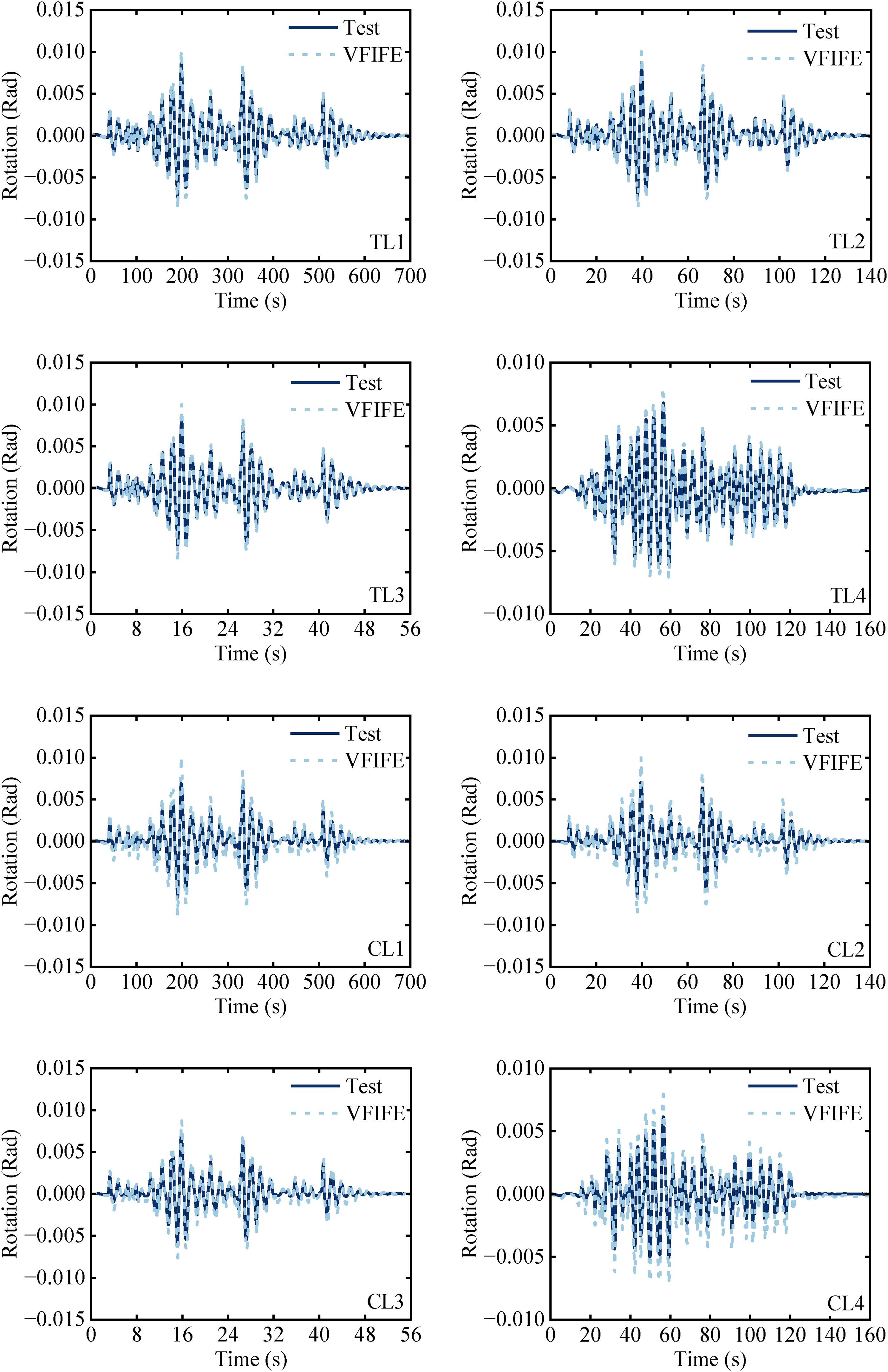
Time history results of gap rotation.

The R² and NRMSE for gap rotation are listed in Table 3. For TL1–TL4, the R² is consistently high, ranging from 97.23% to 97.81%. This shows that the VFIFE predictions are consistent with the experimental data in terms of both amplitude and phase. The model can accurately capture the evolution of rotational gaps during seismic excitation. While for CL1–CL4, the simulated rotations tend to slightly overestimate the experimental values in terms of amplitude. This is reflected in the lower R² values (90.59–95.73%) and a higher NRMSE value (3.98–6.72%). The discrepancies in the cross-shaped joints may be attributed to the redistribution and interaction mechanisms that are not fully captured by traditional simplified modeling assumptions. Additionally, slight differences in boundary conditions, friction, or localized cracking could contribute to the observed discrepancies. In comparison, the simulation successfully replicates the key gap-opening–closing characteristics, demonstrating the advantages of the VL model based on the VFIFE method, which provides a reliable tool for seismic performance evaluation of SC joints.

Table 3.

Coefficient of determination and NRMSE of gap rotation.

Joint type	Case	R² (%)	NRMSE (%)
T-shaped	TL1	97.23	1.38
	TL2	97.81	0.76
	TL3	97.72	1.30
	TL4	97.53	1.78
Cross-shaped	CL1	92.63	3.99
	CL2	95.73	3.98
	CL3	95.87	6.72
	CL4	90.59	6.47

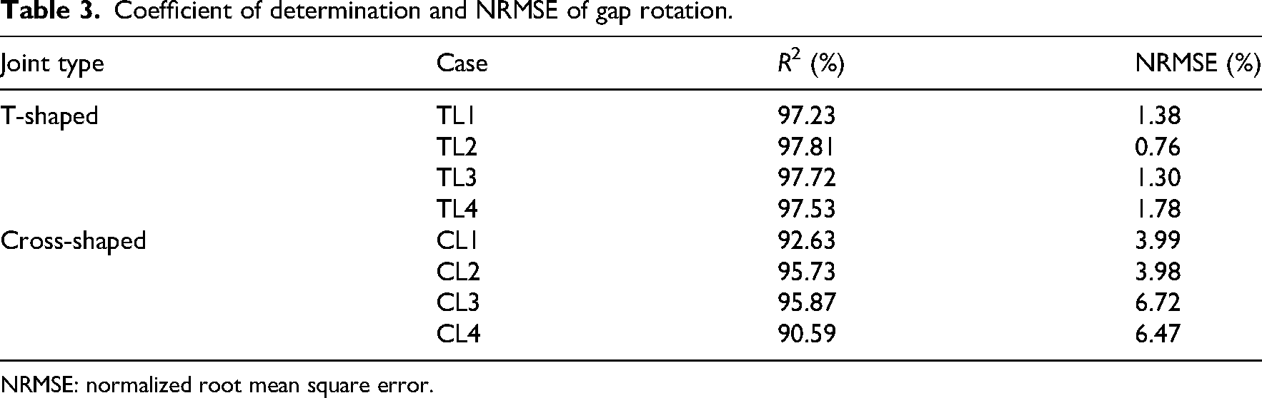
NRMSE: normalized root mean square error.

Tendon force

Tendon force provides the re-centering capability for the SC joint, and its accurate prediction is crucial for evaluating the overall structural behavior. Figure 17 compares the time history responses of the pre-stressed tendon. The VFIFE model (dashed line) successfully captures the overall evolution and phasing of the tendon force when compared to the test data (solid line) across all eight loading cases, accurately tracking the dynamic fluctuations in force throughout the seismic events. Figure 18 shows a direct comparison of maximum and minimum tendon forces. The results show that, while the VFIFE simulation accurately captures the overall behavioral trend, it provides a slightly conservative estimate of peak forces across all eight cases. For instance, in the TL-series, experimental peak forces (29.34–30.15 kN) were under-estimated by the model's prediction (28.59–29.35 kN). This systematic discrepancy is most likely the result of a cumulative effect of idealizations inherent in the simulation. One of the primary assumptions regarding material properties is that the actual elastic modulus of the materials may be higher than the nominal values used in the simulation. These factors, combined with the model's simplified geometry and inability to fully capture complex non-linearities such as concrete micro-cracking, result in lower calculated forces.

Figure 17.

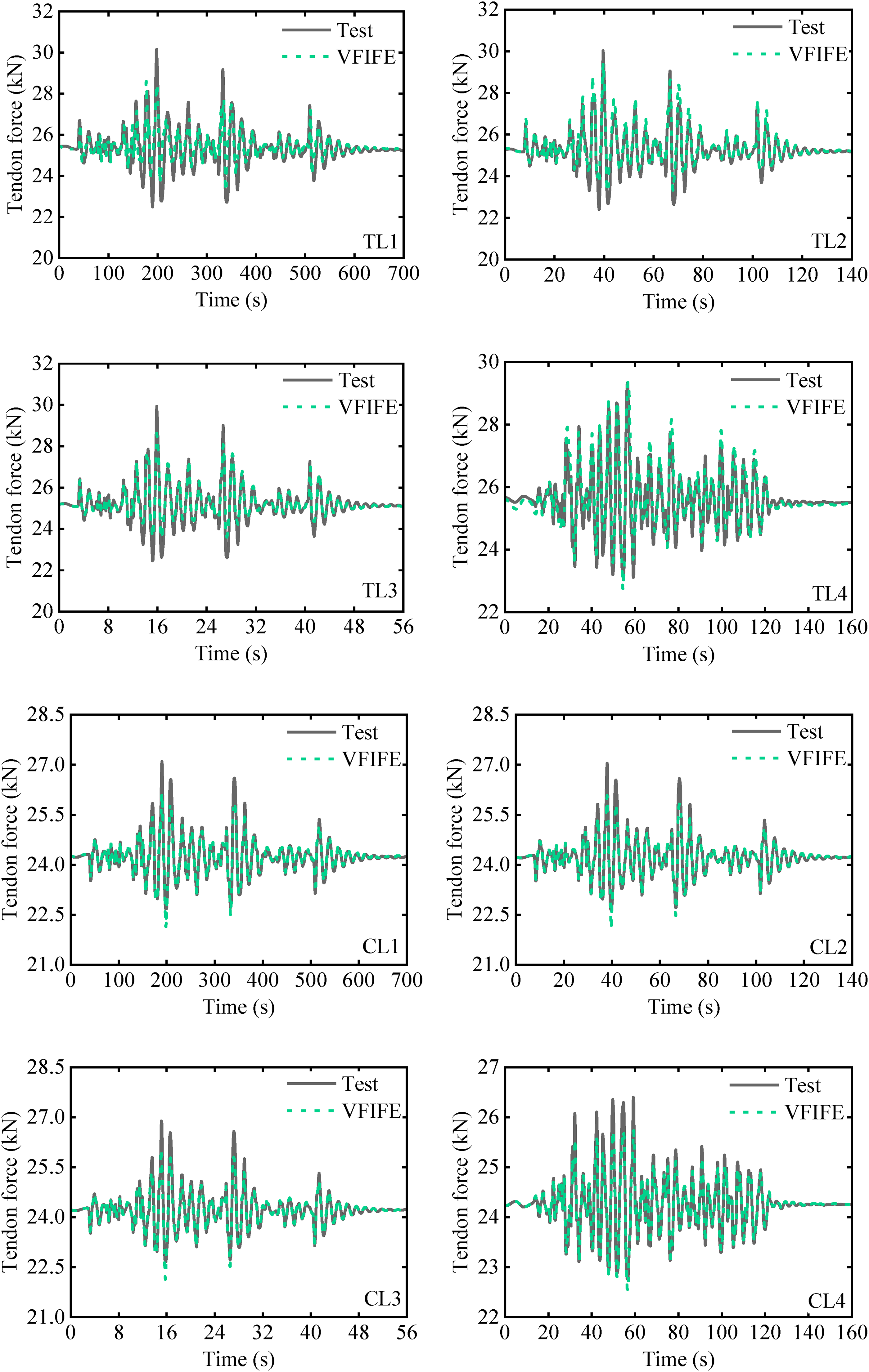
Time history results of tendon forces.

Figure 18.

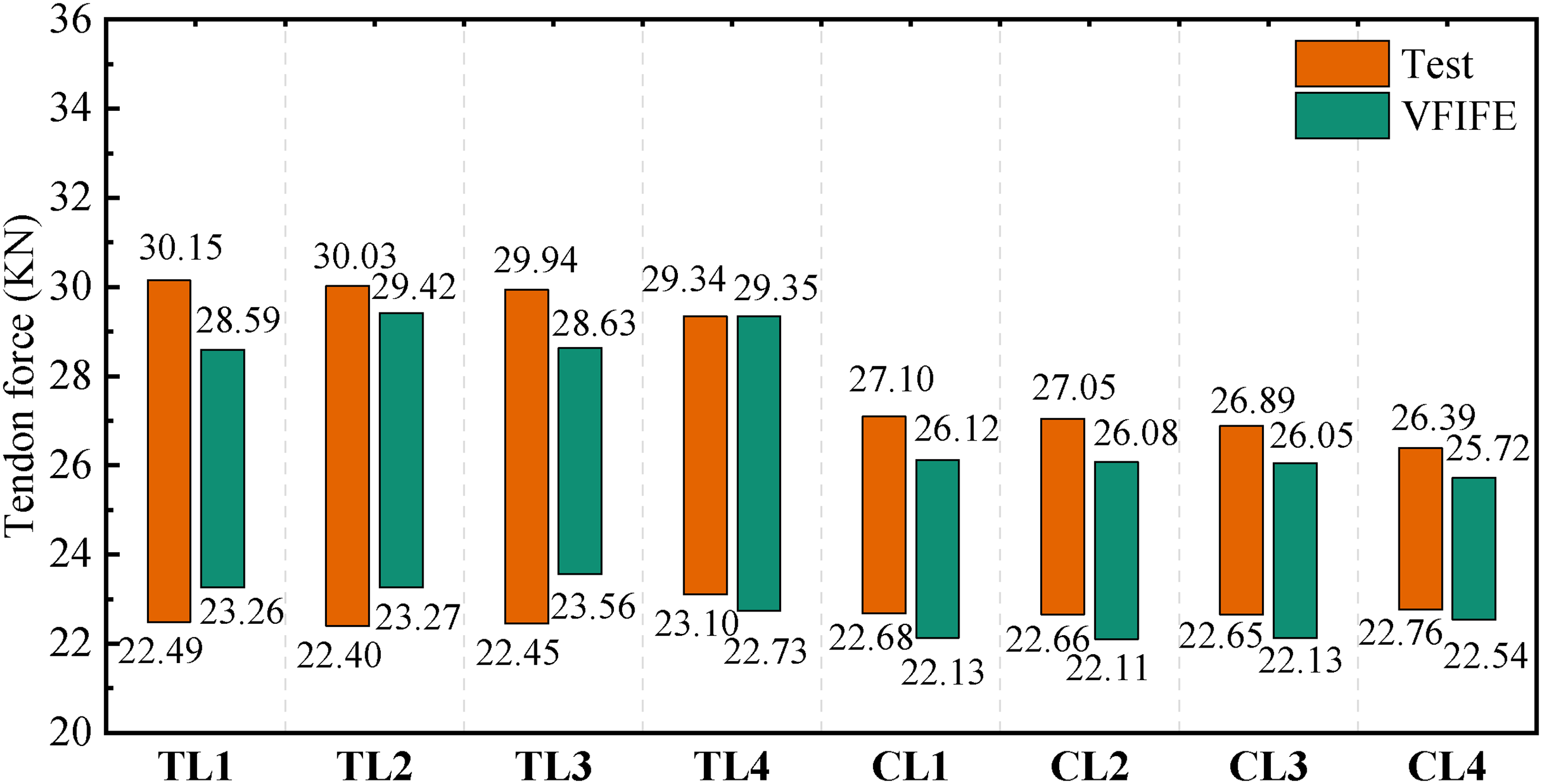
Comparison of tendon force.

Despite these minor differences, the simulation accurately captures the variation in pre-stress within the tendons, which is critical to the joint's seismic performance. This high level of accuracy provides a solid foundation for the design and optimization of SC structures.

Parametric analysis

To further investigate the influence of key design parameters on the seismic performance of SC joints, a parametric study on the initial pre-stressing force of the tendons using the previously validated VFIFE numerical model. The cross-shaped joint model was selected as the subject of analysis, with three different initial pre-stressing forces applied: 20, 30, and 40 kN. By applying a monotonic lateral load to the model, key performance indicators such as joint rotation, residual displacement, and recovery rate were analyzed at different drift angles.

Figure 19 illustrates the relationship between the joint rotation and the drift angle under different pre-stress levels. It is evident from the figure that for the same drift angle, a higher initial pre-stress results in a smaller joint rotation. This is because a higher pre-stressing force increases the initial rotational stiffness of the joint, effectively restraining the opening of the gap between the beam and column, thereby reducing the rotational deformation of the joint.

Figure 19.

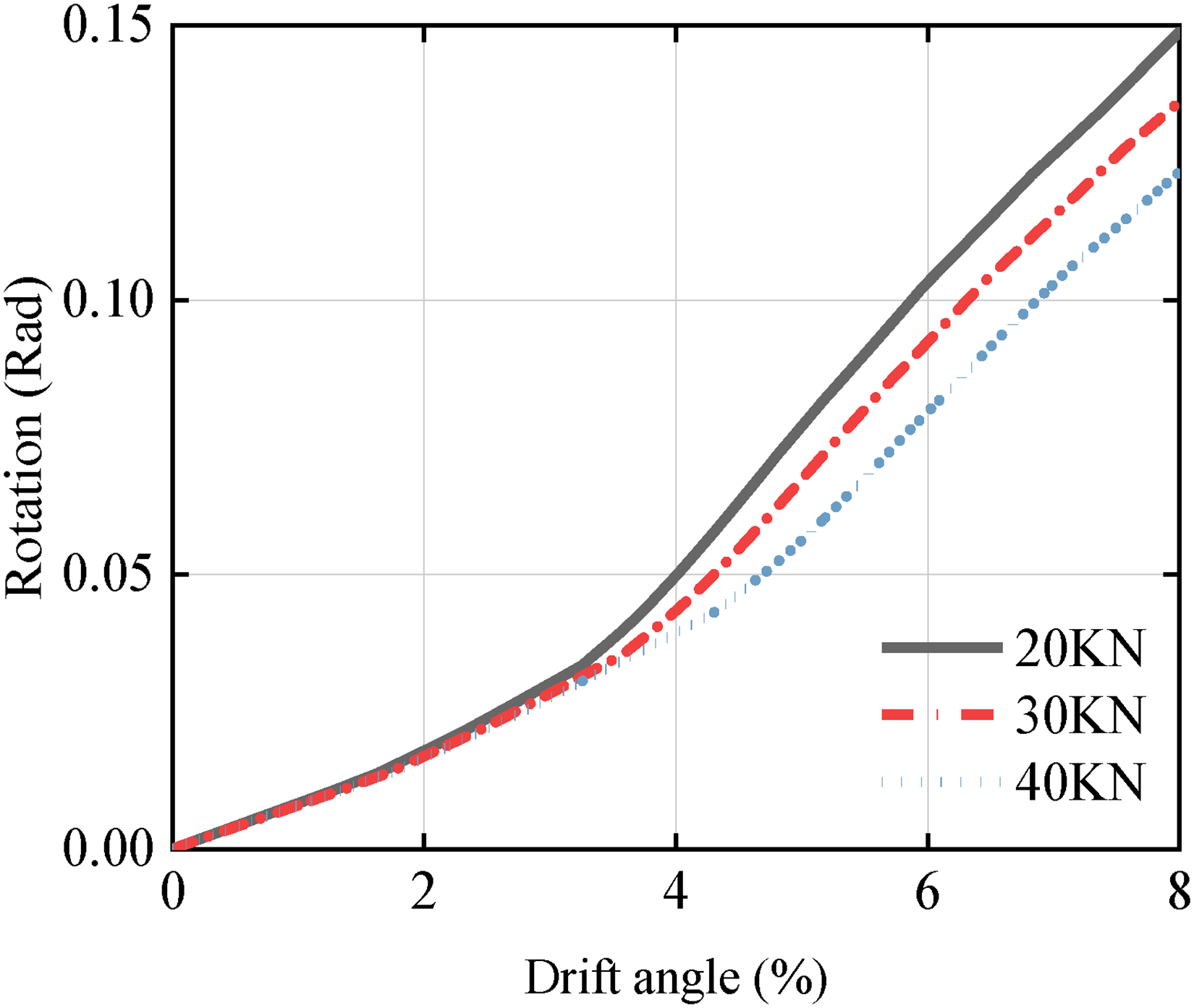
Rotation with different drift angles.

Figure 20 further reveals the effect of the initial pre-stress on the joint's recovery capability. Figure 20(a) shows that at larger drift angles (1/50 and 1/30), the residual displacement of the joint is significantly reduced when a higher initial pre-stress is applied. This indicates that increasing the pre-stress can effectively enhance the SC capability of the joint and reduce the permanent deformation of the structure. The recovery rate curves in Figure 20(b) also confirm this finding. In the figure, a recovery rate of ≥90% is defined as good SC performance, 70–90% as average performance, and <70% as a failure of SC. Under all conditions, the recovery rate is at a “good” level when the drift angle is small. However, as the drift angle increases, the recovery rate of the joint with a lower pre-stress (20 kN) decreases more significantly, whereas the joint with a 40 kN pre-stress maintains a recovery rate of over 90% even at a large drift angle of 1/30.

Figure 20.

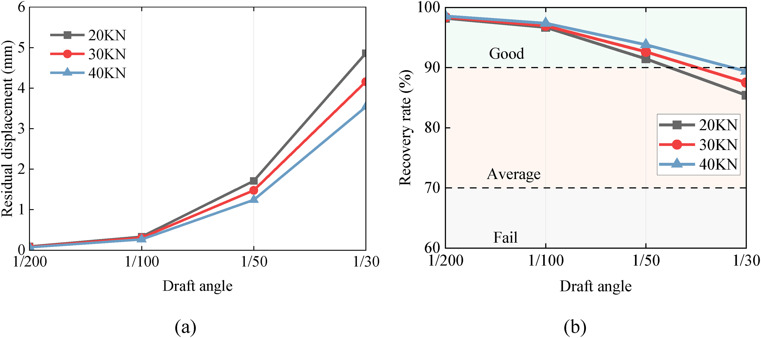
Self-centering ability: (a) residual displacement and (b) recovery rate.

The results indicate that increasing the initial tensioning force of the pre-stressing tendons within a certain range can effectively improve the seismic performance of SC joints. However, it is important to note that a high initial pre-stress can lead to reduced ductility. As shown in Figure 18, if the initial pre-stress is already high, the tendons will reach their yield point after a smaller deformation. Therefore, the trade-off between enhanced SC capability and reduced ductility must be carefully considered during the design process. Given these complex trade-offs, the proposed VL element proves advantageous for future performance-based design optimization. Because of its clear physical parameters and high computational efficiency within the VFIFE framework, engineers can utilize the VL element to conduct large-scale parametric sweeps—such as optimizing the pre-stressed tendon layout and angle steel thickness—through iterative computation, thereby efficiently determining the optimal configuration that maximizes energy dissipation while maintaining a target re-centering ratio.

Conclusions

This study presents a significant advancement in the seismic simulation of SC structures by developing and validating a novel framework based on the VFIFE method and introducing an innovative VL element. The effectiveness of the proposed method was verified through pseudo-dynamic tests. The primary innovations and contributions of this study are summarized as follows:

The proposed VFIFE-based framework provides a robust and unified approach for modeling SC structures. It successfully captures the complex, large-deformation non-linear behaviors inherent in SC joints, including the crucial gap-opening–closing mechanisms and pinching effects, showing excellent correlation with experimental results.

A specialized VL element was developed to directly simulate joint behavior, enabling the precise replication of key performance characteristics under seismic loading. It accurately simulates the joint's gap rotation and the cyclic “energy storage–release” mechanism driven by pre-stressed tendons.

The VL element is designed with inherent flexibility. By simply modifying the geometric layout of the dependent nodes and updating the constitutive laws, this element can be easily extended to simulate other gap-opening structures, such as the rocking toe mechanisms in rocking walls or the unbonded dry joints in precast segmental bridge columns, highlighting its broad application potential.

Footnotes

ORCID iDs

Hongmei Zhang

Maolin Tian

Yuanfeng Duan

Fan Hu

Yi Fang

Yuanzheng Wang

Author contributions

Hongmei Zhang: conceptualization, funding acquisition, methodology supervision, and writing—review and editing. Maolin Tian: writing—original draft, data curation, investigation, and validation. Yuanfeng Duan: supervision, funding acquisition, and writing—review and editing. Fan Hu: formal analysis and validation. Yi Fang: writing—review and editing and validation. Yuanzheng Wang: validation.

Funding

The authors disclosed receipt of the following financial support for the research, authorship, and/or publication of this article: This research was funded by the Zhejiang Provincial Natural Science Foundation of China (Grant No. LHZ23E08003), and the National Natural Science Foundation of China (Grant Nos. 52378540, 52361165658, and U24A20169).

Declaration of conflicting interests

The authors declared no potential conflicts of interest with respect to the research, authorship, and/or publication of this article.

Data availability statement

The data will be made available upon reasonable request.

References

Chancellor

Eatherton

Roke

, et al. (2014) Self-centering seismic lateral force resisting systems: High performance structures for the city of tomorrow. Buildings 4(3): 520–548.

Cheng

C-T

(2008) Shaking table tests of a self-centering designed bridge substructure. Engineering Structures 30(12): 3426–3433.

Chou

C-C

Chen

J-H

(2011) Seismic design and shake table tests of a steel post-tensioned self-centering moment frame with a slab accommodating frame expansion. Earthquake Engineering and Structural Dynamics 40(11): 1241–1261.

Cui

Jiang

(2017) Experimental investigation of tri-axial self-centering reinforced concrete frame structures through shaking table tests. Engineering Structures 132: 684–694.

Deng

Pan

Lam

, et al. (2013) Test and simulation of full-scale self-centering beam-to-column connection. Earthquake Engineering and Engineering Vibration 12(4): 599–607.

Dong

, et al. (2024) Nonlinear dynamic collapse analysis of space semi-rigid frames using finite particle method. Journal of Constructional Steel Research 216: 108607.

Dou

(2025) Cyclic loading behavior of earthquake-resilient disc-spring self-centering beam-column joints: An experimental study. Engineering Structures 335: 120366.

Duan

Zhang

, et al. (2014) Entire-process simulation of earthquake-induced collapse of a mockup cable-stayed bridge by vector form intrinsic finite element (VFIFE) method. Advances in Structural Engineering 17(3): 347–360.

Duan

Tao

Zhang

, et al. (2019) Real-time hybrid simulation based on vector form intrinsic finite element and field programmable gate array. Structural Control and Health Monitoring 26(1): e2277.

10.

Duan

Tian

Zhang

, et al. (2025) An innovative vector mechanics approach for prestressed concrete beam. International Journal of Structural Stability and Dynamics 25(24): 2540028.

11.

Dyanati

Huang

Roke

(2017) Cost-benefit evaluation of self-centring concentrically braced frames considering uncertainties. Structure and Infrastructure Engineering 13(5): 537–553.

12.

Fang

Qiu

Wang

, et al. (2023) Self-centering structures against earthquakes: A critical review. Journal of Earthquake Engineering 27(15): 4354–4389.

13.

Fraternali

Santos

(2019) Mechanical modeling of superelastic tensegrity braces for earthquake-proof structures. Extreme Mechanics Letters 33: 100578.

14.

Garlock

Ricles

Sause

(2003) Cyclic load tests and analysis of bolted top-and-seat angle connections. Journal of Structural Engineering 129(12): 1615–1625.

15.

Guo

Song

Zhang

(2011) Numerical simulation of the seismic behavior of self-centering steel beam–column connections with bottom flange friction devices. Earthquake Engineering and Engineering Vibration 10(2): 229–238.

16.

Haque

Issa

Shahria Alam

(2019) Superelastic shape memory alloy flag-shaped hysteresis model with sliding response from residual deformation: Experimental and numerical study. Journal of Intelligent Material Systems and Structures 30(12): 1823–1849.

17.

Hou

Fang

Zhang

(2018) Static contact analysis of spiral bevel gear based on modified VFIFE (vector form intrinsic finite element) method. Applied Mathematical Modelling 60: 192–207.

18.

Jia

Zhang

Zeng

, et al. (2022) Effect of loading rate and initial strain on seismic performance of an innovative self-centering SMA brace. Materials 15(3): 1234.

19.

Jiang

(2018) Simulation of contact surfaces in self-centering reinforced concrete frames with test validation. In: Hordijk

Luković

(eds) High Tech Concrete: Where Technology and Engineering Meet. Cham: Springer International Publishing, 1209–1216.

20.

Kent

Park

(1971) Flexural members with confined concrete. Journal of the Structural Division 97(7): 1969–1990.

21.

Kim

H-J

Christopoulos

(2009) Seismic design procedure and seismic response of post-tensioned self-centering steel frames. Earthquake Engineering & Structural Dynamics 38(3): 355–376.

22.

Zhao

Sun

, et al. (2025) Numerical simulation approach and seismic performance investigation of self-centering precast concrete frames. Soil Dynamics and Earthquake Engineering 190: 109172.

23.

Lin

Luo

Tang

, et al. (2022) A fiber beam element for the finite particle method considering shear and torsion deformation. Engineering Mechanics 39(5): 34–43.

24.

Liu

Lin

(2016) Simulation of a buried pipeline crossing strike-slip fault based on vector form intrinsic finite element (VFIFE) method with fiber element model. In: The 26th International ocean and polar engineering conference.

25.

Cui

Liu

, et al. (2015) Shaking table test and numerical simulation of a 1/2-scale self-centering reinforced concrete frame. Earthquake Engineering and Structural Dynamics 44(12): 1899–1917.

26.

Menegotto

(1973) Method of analysis for cyclically loaded R. C. Plane frames including changes in geometry and non-elastic behavior of elements under combined normal force and bending. Proceedings of IABSE symposium on resistance and ultimate deformability of structures acted on by well defined repeated loads. Epub ahead of print 1973.

27.

Moradi

Alam

(2015) Feasibility study of utilizing superelastic shape memory alloy plates in steel beam–column connections for improved seismic performance. Journal of Intelligent Material Systems and Structures 26(4): 463–475.

28.

Pampanin

(2012) Living a new era in earthquake engineering: Targeting damage-resisting solutions to meet societal expectations. In: Australian Earthquake Engineering Society 2012 conference, p. 7–9.

29.

Ping

Fang

Chen

, et al. (2021) Seismic robustness of self-centering braced frames suffering tendon failure. Earthquake Engineering and Structural Dynamics 50(6): 1671–1691.

30.

Resapu

Perumahanthi

(2021) Numerical study of bilinear isotropic & kinematic elastic–plastic response under cyclic loading. Materials Today Proceedings 39: 1647–1654.

31.

Ruiz-Pinilla

Adam

Pérez-Cárcel

, et al. (2016) Learning from RC building structures damaged by the earthquake in Lorca, Spain, in 2011. Engineering Failure Analysis 68: 76–86.

32.

Scott

Park

Priestley

MJN

(1982) Stress–strain behavior of concrete confined by overlapping hoops at low and high strain rates. Journal of the American Concrete Institute 79(1): 13–27.

33.

Shen

P-W

Yang

Hong

J-H

, et al. (2020) Seismic performance of steel frame with a self-centering beam. Journal of Constructional Steel Research 175: 106349.

34.

Shih

Wang

Y-K

Ting

(2004) Fundamentals of a vector form intrinsic finite element: Part III. Convected material frame and examples. Journal of Mechanics 20(2): 133–143.

35.

Song

Guo

Chen

(2014) Experimental and numerical study of a self-centering prestressed concrete moment resisting frame connection with bolted web friction devices. Earthquake Engineering and Structural Dynamics 43(4): 529–545.

36.

Song

L-L

Guo

Cao

Z-L

(2015) Seismic response of self-centering prestressed concrete moment resisting frames with web friction devices. Soil Dynamics and Earthquake Engineering 71: 151–162.

37.

Ting

Shih

Wang

Y-K

(2004a) Fundamentals of a vector form intrinsic finite element: Part I. Basic procedure and a plane frame element. Journal of Mechanics 20(2): 113–122.

38.

Ting

Shih

Wang

Y-K

(2004b) Fundamentals of a vector form intrinsic finite element: Part II. Plane solid elements. Journal of Mechanics 20(2): 123–132.

39.

Wang

Zhu

Qiu

C-X

, et al. (2019) High-performance self-centering steel columns with shape memory alloy bolts: Design procedure and experimental evaluation. Engineering Structures 182: 446–458.

40.

, et al. (2023) Seismic performance of full-scale self-centering reinforced concrete beam–column joints: Experimental, numerical and theoretical analysis. Journal of Building Engineering 78: 107683.

41.

Guo

Hao

, et al. (2026) Engineering resilience through hierarchical isolation: A mega-frame with sub-structure isolation system. Structures 85: 111312.

42.

Xue

Chen

, et al. (2009) Post-earthquake loss assessment based on structural component damage inspection for residential RC buildings. Engineering Structures 31(12): 2947–2953.

43.

Yan

Shi

Mao

, et al. (2024) Seismic response of prestressed self-centering moment-resisting frames. Buildings 14(12): 3811.

44.

Yang

Zhu

, et al. (2025) Seismic performance of steel frames with different configurations of self-centering joints. Structures 74: 108480.

45.

Yashinsky

(2005) Earthquake damage to structures. In: Chen

Liu

(eds) Earthquake Engineering for Structural Design. Boca Raton: CRC Press, 46–103.

46.

Zhang

Fang

Cao

, et al. (2025) Shaking table investigation of pulse-type seismic behavior of a self-centering reinforced concrete frame structure. Engineering Structures 325: 119417.

47.

Zhang

Duan

, et al. (2025) A vision-based deformation tracking for self-centering structures during shaking table tests. Engineering Structures 330: 119800.

48.

Zhong

Christopoulos

(2022) Self-centering seismic-resistant structures: Historical overview and state-of-the-art. Earthquake Spectra 38(2): 1321–1356.