
Abstract
We deal with a retailer’s multi-product inventory system where customers randomly seek acceptable substitutes if their initial requests are not satisfied. Unsuccessful quests for substitutes would result in lost sales. Motivated by a consulting project as well as other real practices, we also choose to deal with further challenges posed by initially unknown base demand distributions and substitution probabilities; moreover, we aim to develop an offline learning method that (i) takes advantage of given data derived from bygone decisions rather than of any learning-while-doing opportunity, (ii) makes inferences about base-demand distributions and pairwise substitution probabilities without knowing whether there have been demand arrivals after inventory depletions, and (iii) is unhindered by the lack of knowledge about the assortments faced by customers and their purchase-or-no-purchase decisions at their individual arrivals. To address these challenges, we propose an innovative approach based on the Kaplan-Meier estimator that circumvents unrealistic data requirements. Our substitution probability estimates employ carefully designed weighting schemes to facilitate rigorous theoretical analysis through tools such as the Cauchy-Schwartz inequality. Both one-time substitution scenarios and more complex Markov-chain substitution patterns would be accommodated. Using large deviation tools, we establish provably optimal convergence rates of our estimates on top of consistency. The precision in parameter estimates would translate into accuracy in replenishment decisions. For inventory management, we take advantage of a submodularity property to obtain an exact algorithm for the two-product case and a good heuristic for the general multi-product problem. Computational studies based on simulated and actual data confirm the merits of our approach.
Introduction
Lost sales figure prominently in retailers’ day-to-day operations. Approximately $984B out of the world’s $28.64T retail turnover is lost to stockouts (Buzek, 2018; eMarketer, 2022). Among them, as much as 47% are attributed to inadequacies in store-level forecasting and replenishment (Gruen and Corsten, 2007). On the flip side, stockouts are not always detrimental. They may prevent spoilage and induce substitution demands for more profitable products (Zhang et al., 2021).
Within this context, we investigate learning methods of demand patterns and substitution behaviors, with some attention also paid to the optimization portion after parameter learning. Besides censoring which has long plagued demand learning involving lost sales, we face the additional challenge stemming from our data being intertwined with the concerned retailer’s past replenishment activities that are beyond our control. In addition, our applications demand us to estimate all pair-wise substitution probabilities directly instead of assessing potentially much fewer behind-the-scenes parameters that prop up the substitution behaviors.
Motivation by a Large European Chain
A European grocery chain has several hundred stores that are supplied with various breads from ten production facilities. Every store in the chain places and receives orders for a variety of fresh bread types before its daily opening. Any remaining stock at the end of a day is scrapped.
The store faces inaccurate demand information for each stock-keeping unit (SKU), while the stockout of one SKU induces the censoring of its own demand and substitution requests being made to one or more other SKUs. Further complicating the problem is that substitution probabilities are unknown and must be estimated along with the original base demand per SKU. One might think that a positive stock level at the end of the day would allow the true demand to be captured by that day’s sales records; however, some of the sales for that SKU might originate from other products that have run out of stock. In other words, observed sales are not true demand: the stockout of one product causes not only the censoring of its own demand but also a distortion of the demands for its substitutable products.
To better monitor the substitution-induced demand generated by stockouts, the company split the business period into hourly blocks and recorded the stores’ inventory levels at the beginning of each block. It gave us one year’s worth of historical sales and stock data at one of its stores, and then asked us to make forecasts, identify substitutions, and suggest replenishment quantities for the stores.
Figure 1 illustrates the store’s demand pattern. It involves
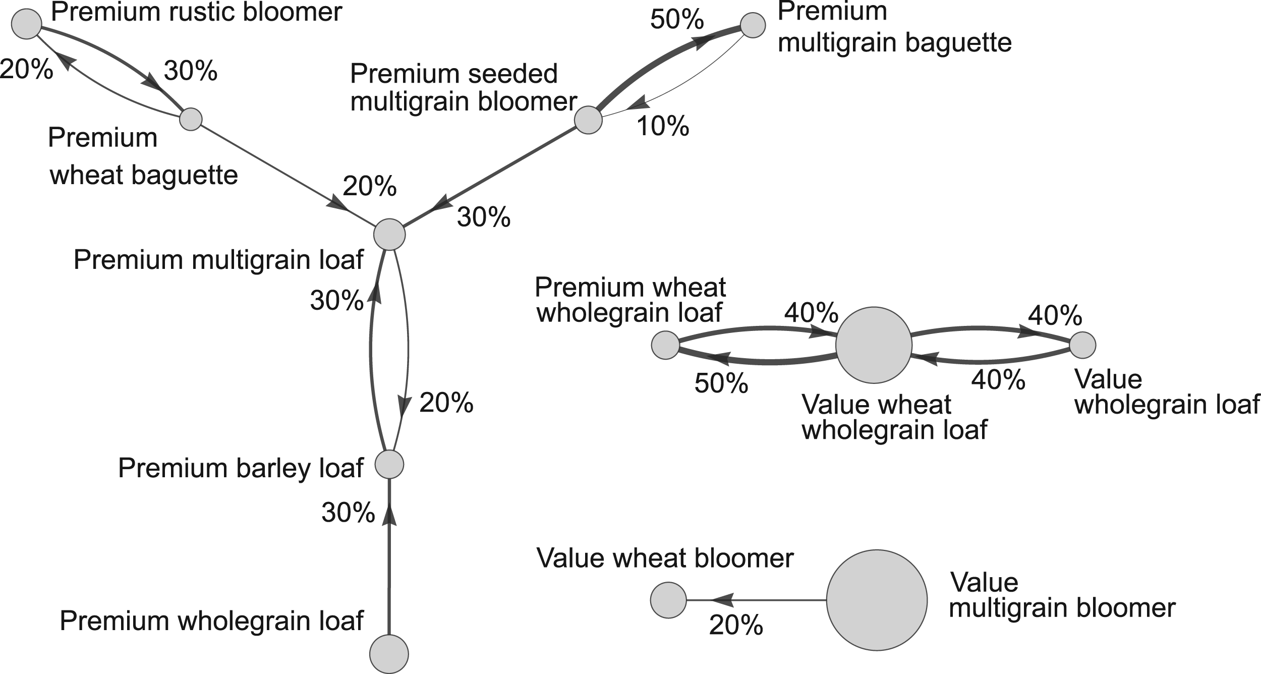
A rough pattern of product substitutions.
In Figure 1, substitutions are limited to product clusters, with the largest involving seven products. For instance, a shortage of Value multigrain bloomer would call for the help of Value wheat bloomer, while no other shortage would affect this product. We may observe two key patterns: (1) not all pairs of products have substitution relationships; and (2) the substitution frequencies are not correlated with the concerned products’ average historical sales. These prompt us to build a model wherein each product has a base demand and when a stockout occurs, customers seek out alternatives following certain probabilities. This probability-based substitution approach is well-known in inventory management; see, for example, Netessine and Rudi (2003), Nagarajan and Rajagopalan (2008), Zhang et al. (2021), and Chen and Chao (2020).
We recognize that discrete choice models are frequently used for multi-product operations management. They typically require detailed sales data that cover (1) assortments faced by customers at their arrivals and (2) customers’ no-purchase decisions; see, for example, Şimşek and Topaloglu (2018) and Chen et al. (2022). Unfortunately, such detailed transaction-level data are unavailable to the European grocery chain. Therefore, estimations based on choice models are unsuitable for the current problem, as well as other problems with only aggregate sales data.
Some works like Newman et al. (2014) and Abdallah and Vulcano (2021) made efforts to circumvent the need for observing no-purchase decisions. Still, they had to assume knowledge of assortments at various transactions, special demand arrival patterns like Poisson, and parametric substitution behaviors like multinomial logit (MNL). The latter works rely on the independence of irrelevant alternatives (IIA), which is violated by our European chain as shown in Figure 1. For instance, a shortage of Value multigrain bloomer would call for the help of Value wheat bloomer, which is not affected by the shortage of any other product.
In contrast, using merely inventory-level records at pre-fixed time points, our method can estimate base-demand distributions and substitution probabilities without being constrained by any pre-set conditions. The added flexibility renders it applicable to many real-world scenarios where available data are not ideal.
For ease of exposition, we start our research with two products. In this setting, a retailer decides period-wise (e.g., daily) replenishment quantities for two substitutable products. Demands for the two products arrive in fashions initially unknown to the retailer. A request for one of the products, if unsatisfied, translates into a request for the other product at a probability that is again initially unknown.
To gain information about the demands, the retailer tallies sales and inventory levels at certain checkpoints during the period—any two consecutive checkpoints help mark out a block (e.g., an hour). The early blocks of a period are rarely affected by stockouts and they therefore aid the learning of pre-substitution base demand distributions. Meanwhile, stockouts and substitutions are more rampant in later blocks which could help us to better assess substitution probabilities.
Block-wise sales and inventory data are fed to a Kaplan–Meier (KM)-type estimator to generate demand estimates in the face of censoring enforced so strictly that even knowledge about whether there has been any demand arrival after the depletion of an inventory is not available. We then estimate substitution probabilities by taking ratios between KM-estimated substitution realizations and estimated substitution requests. Certain carefully designed weights are applied to the ratio-forming formulae to help the estimates’ convergence. By regret in this learning-then-optimization regime, we mean the difference between the optimal per-period profit achievable under true problem parameters and that achievable under the estimated ones.
Using large-deviation tools and information-theoretic techniques, we can verify our learning method’s attainment of tight regret bounds. We also work on the effective computation of optimal replenishment levels under known problem parameters. Here, some innate submodularity is exploited. All our results are extendable to the multi-product case. Here, an implicit assumption is that each customer encountering a stockout would attempt substitution for just once. Such one-time substitutions have been widely adopted in inventory management; see, for example, Netessine and Rudi (2003) and Nagarajan and Rajagopalan (2008).
We also consider the extension to a Markov-chain substitution model, allowing customers to attempt multiple substitutions in a Markov chain fashion. Even though discrete choice models are unsuitable for our learning problem as has already been discussed, we draw our inspiration drawn from the Markov-chain choice model of Blanchet et al. (2016) and Şimşek and Topaloglu (2018). While having fewer spelled-out coefficients, the regret bound that we can achieve for multi-product Markov-chain substitution has nevertheless the same order of time growth as that for one-time substitution.
Contributions and Key Results
This work is inspired by the industry’s need to understand problem parameters ranging from base demand distributions to pair-wise substitution probabilities. Worthy of note are three features: The learning must work for a given historical data set, which may be devoid of any opportunity to place exploration-intended orders. This distinguishes us from Chen and Chao (2020), who also estimated both demand distributions and substitution probabilities, albeit with the freedom to manipulate orders for active learning purposes. Incidentally, to the best of our knowledge, this work is the only one other than ours that deals simultaneously with the learning of substitution probabilities and operations optimization involving demand learning. While Chen and Chao (2020) took on learning-while-doing challenges, we consider a complementary situation where replenishment decisions reflected in the data are already bygone. We do not insist on knowing whether there have been demand arrivals after the occurrences of stockouts; hence, our treatment of censoring is in a sense more thorough. Our KM estimation has made improvements on that of Huh et al. (2011), who still required what we call the strong censoring indicators on post-depletion demand arrivals. Although insignificant for a continuous-demand case, not needing any post-depletion information could help greatly expand our method’s applicability when demands are discrete. Our data form is not compatible with estimations based on choice models. Such methods typically require information on both assortments at various purchase occasions and customers’ purchase-or-no-purchase decisions. Our aggregate inventory-sales data do not hold such information. This propels our approach to be fundamentally different from existing estimation methods for choice models. This being said, we do draw inspiration from the state-of-the-art Markov-chain choice model of Blanchet et al. (2016) in our extension to a Markov-chain substitution model.
Also notable is the fact that our data are granular at block-wise levels. Although Jain et al. (2014) estimated demand distributions from block-wise demand, they did not provide the means to extract substitution probabilities from the block-wise estimates. This turns out to be a nontrivial task.
Performance guarantees
Our learning approach leads to base demand distributions and substitution probabilities that converge to their true values. Using large deviation theory, we can derive exponential convergence rates of the demand-related parameters; see Theorem 1. This result then extends to an
Submodularity and optimization
Beyond the known submodularity of the profit function under proportional substitution (Netessine and Rudi, 2003; Zhang et al., 2021), we achieve the same property for stochastic substitution; see Theorem 3. Maximization of a submodular objective function remains NP-hard (Bian et al., 2017: Proposition 5). Nevertheless, a double greedy heuristic exists for proportional substitution (Zhang et al., 2021), which is polynomial in the number of products. This heuristic is also applicable to our multi-product problem with probabilistic substitutions.
This work builds upon existing research in optimal inventory management for multiple mutually substitutable products. A common model in this field assumes that when a stockout occurs for a product, customers may choose another product as a substitute based on known exogenous probabilities or proportions. Numerous studies have focused on characterizing the structural properties of optimal inventory policies when both the demand distribution and customers’ substitution probabilities are known to the retailer.
Nagarajan and Rajagopalan (2008) investigated optimal inventory policies for substitutable products and introduced a partially decoupled base-stock policy. Schlapp and Fleischmann (2018) analyzed a multi-product model with capacity constraints, focusing on the effects of capacity limits and substitution preferences. Additionally, Zhang et al. (2021) formulated a multi-product inventory problem as an integer program and derived necessary optimality conditions.
Instead of the management aspect, our research concentrates on learning the demand distributions and substitution probabilities directly from the retailer’s historical sales data. We develop an effective offline learning algorithm and demonstrate its theoretical convergence properties. By enabling data-driven inventory decisions, this approach provides a practical framework for retailers to determine optimal inventory levels based on past sales records.
Many works utilize choice models to capture substitution effects. These include MNL (Vulcano et al., 2012), nested logit (Kök and Xu, 2011), and the Markov-chain choice model (Blanchet et al., 2016). Estimations of such models’ parameters usually require knowledge on real-time assortment evolutions and customers’ no-purchase decisions. Such information is not derivable from the aggregate inventory-sales data provided to us. We are thus compelled to come up with fundamentally different approaches than those based on choice modeling.
When retailers only have transaction data instead of complete information about the demand and substitution structures while the data themselves are likely incomplete, many researchers used the expectation–maximization (EM) method to recover the true demand-related information; see Anupindi et al. (1998). Apart from EM, competing approaches existed in the forms of likelihood estimation (Newman et al., 2014) and Markov chain Monte Carlo methods (Musalem et al., 2010). Unlike these approaches, we make adaptations to the renowned KM estimator. These enable us to estimate demand distributions without any prior assumptions, widening the applicabilities of our approach.
The KM estimator and its product-limit form were proposed by Kaplan and Meier (1958). They are widely used in survival analyses and medical trials. Foldes and Rejto (1981) showed the convergence of the KM estimator under random independent censoring. We use a similar method to estimate demand distributions. In our current situation, the conventional assumptions of independence are no longer realistic. Our theoretical derivations benefit from Huh et al. (2011), who allowed censoring variables to depend on past observations as well. However, we have no use of some strong censoring indicators needed by them which essentially tell whether more demand requests arrive after inventories have been emptied.
We also contribute to data-driven inventory control. For a single-product case, Levi et al. (2007) used uncensored empirical distributions to approximate true distributions and gave performance bounds. Huh and Rusmevichientong (2009) dealt with lost sales and demand censoring using a gradient-descent algorithm. Besbes and Muharremoglu (2013) designed an exploration-exploitation algorithm with a provable regret bound. For inventory management with lead time, Zhang et al. (2020) leveraged the convexity of the profit function and developed an online learning algorithm, while Lyu et al. (2024) integrated the upper confidence bound algorithm with the KM estimator. In multi-product settings, Shi et al. (2016) considered warehouse capacity constraints and applied online convex optimization techniques to the learning of inventory levels from data. To this growing body of literature, we add our approach to stockout-based substitutions involving demand learning from aggregate inventory sales data.
In their learning-while-doing study of a multi-product inventory control problem, Chen and Chao (2020) made the same stochastic-substitution assumption as ours. Having its own challenges notwithstanding, this earlier work possesses a unique advantage over ours: the ability to manipulate replenishment quantities for the purpose of data collection. Indeed, Chen and Chao (2020) took this advantage to its fullest extent by using their exploration-then-exploitation stages that grow in lengths in a doubly exponential fashion. Within each exploration phase, they cleverly inflated replenishments. Moreover, they cycled through the products, deliberately under-supplying one product a time to extract information on substitution activities. Their analysis was also assisted by the assumption that cost- and demand-related parameters would together allow an
In contrast, we take a vastly different approach to our past and hence no-longer-manipulable data in order to extract useful information for profit optimization purposes. The fact that data comes in a block-wise fashion has helped us tremendously. There are ample opportunities for high inventory levels to dampen the censoring effects and for low inventory levels to reveal the substitution effects. For the former, we enlist the help of KM estimation instead of simple averages of sales data. Our assumptions on demand-related parameters, though considerably strong, are not interwoven with those regarding cost-related parameters. Consequently, the derivation of our performance bounds relies on intricate arguments afforded by close scrutinies of the profit function itself. Aside from demand learning, we derive the latter’s submodularity and make efforts to efficiently solve the optimization problem that may have multiple local optima.
Problem Formulation
For the ease of presentation, let us start with two products. Our retailer sells two substitutable products with given sales prices and unit costs. Any customer facing stockout independently decides whether or not to seek substitution from the other product. Any still-unmet demand is lost. The retailer begins without prior knowledge about demand distributions or substitution probabilities. However, historical stock levels and sales data for the two products are available.
Let us use the term period to denote a replenishment cycle. It is further decomposed into business selling blocks, much as a day can be divided into hours. Each product is allowed one single inbound delivery at the beginning of every period. The retailer can observe the stock level at the beginning of each block and make deductions about block-wise sales levels. He can neither observe unmet demand nor tell whether a sales event emanates from an originally intended purchase or a substitution attempt.
The retailer sells a set of
Although the exact demand upper bounds may not be precisely known, firms usually possess reasonable prior knowledge of their likely magnitudes. For instance, brick-and-mortar retailers often estimate customer populations and preferences through field surveys or market research that provide practical benchmarks for inventory decisions. Hence, firms likely maintain working estimates of plausible demand upper bounds. Alternatively, firms may glean information about the demand upper bounds from historical sales data.
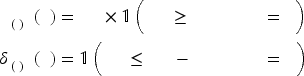
We also let fixed substitution probabilities
We acknowledge that in more realistic settings, substitution behavior may vary across customer segments, product attributes, or temporal factors such as promotions and seasonality. Allowing substitution probabilities to evolve with these contextual variables would better capture such behavioral heterogeneity. However, we adopt fixed substitution probabilities here for theoretical tractability and to isolate the effects of censored observations on learning and optimization performance. Extending the framework to accommodate feature-based or segment-aware substitution models represents an important direction for future research, which we further discuss in the conclusion.
Unlike conventional models, neither any
Also following (1), the total composite demand for product


For some

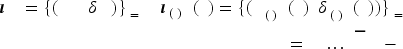
Formally, we name the
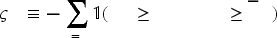
Owing to lost sales and the resulting censoring, we can only access the sales data

We first introduce the original KM estimator and then present our KM-based estimation.
Fundamentals of KM Estimation
The KM estimator was introduced six decades ago by Kaplan and Meier (1958) for constructing empirical CDFs from censored data sets.
Let
We may sort the observations
When every
For an example, suppose
When
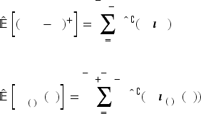
Let us follow the convention of Section 4.1 to express expectations with respect to the KM-estimated distributions using
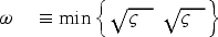
The estimation accuracy for
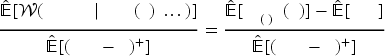
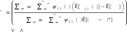
To emulate the two terms regarding base demands in (8), also let
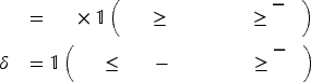
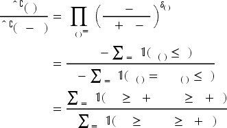
Following (2), we shall weigh (8)’s terms using the
In detail, our procedure works as follows:
We use
Moreover, we use
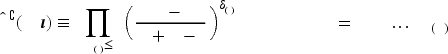
Now, we have posets for each product
Using (7), we compute the KM-estimated CCDF for each product

We calculate the expectations for the block-wise base and composite demands using the CCDFs estimated from the posets, for
In
Under reasonable conditions, we prove the convergence of the KM-based estimates for both base demand distributions and substitution probabilities. This result leads us to a regret bound concerning the replenishment problem. The bound is shown to be tight. Submodularity, in turn, enables a greedy algorithm.
Convergence of Estimators
We first make an assumption on the random nature of historical replenishment levels
The order-up-to level
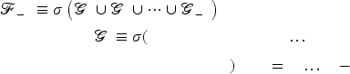
The filtration
We also impose an assumption about the block-wise demand levels.
For any product
In Assumption 2,
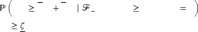
Recall that the retailer can only control the first block’s starting inventory levels
For some strictly positive constants
Assumption 3 imposes bounds on the retailer’s order-up-to levels in period
Besides, as long as the unit sales prices are not outrageously higher than the unit ordering costs, a back-of-the-envelope calculation using the newsvendor formula indicates that order-up-to levels should not be too high. Second, even if the inequalities inside the probabilities point to unwise decisions, we should still give a real-life retailer some allowance for occasional mistakes.
While Assumption 1 is impossible to verify numerically, we have provided partial validations in Section 7.2 for Assumptions 2 and 3 using real data from the European grocery chain.
We are now in a position for an intermediate result.
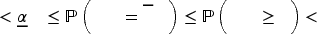
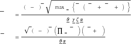
Based on Assumptions 1 to 3, we can define strictly positive constants for any period for any product for any product
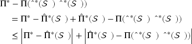
In Proposition 1, part
The proposition is itself sufficient but not exactly necessary. In Sections 7.1.1 and 7.1.2, we shall deliberately inflate the demand upper bounds and approximate them using different sales quantiles, respectively. The results show that our estimation-optimization framework is robust under mis-specifications.
Let us now derive the convergence of our estimates.
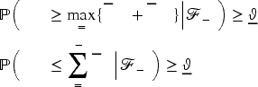
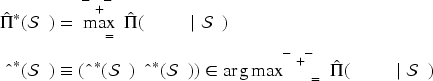
The following statements are true: (Convergence of the demand distribution) For any (Convergence of the substitution probability) For any
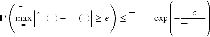
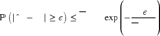
We now provide a sketch of Theorem 1’s proof. To establish the convergence of the estimated demand distribution, let us focus on the KM-estimated CCDF,
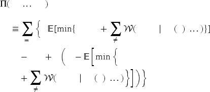
We rely on the decomposition that

When it comes to the substitution probabilities, we note from (2) and (12) that both the true and estimated substitution probabilities are in a fractional form. Simplifying the true and estimated substitution probabilities by
All detailed proofs for this section are in Appendix B of the E-Companion. We not only prove the convergence of KM estimators as was done by Huh et al. (2011) but also identify convergence rates for the demand distributions and substitution probabilities. The
Convergence of the Profit Function
With the estimated demand distributions and substitution probabilities given, our retailer can determine optimal replenishment quantities. To describe the problem that he faces, let
This may appear as a one-shot problem. However, with each salvage value
Due to the peculiar natures of a Markov decision process as implied by (18) and the fact from (19) that
Since we can only access the data set
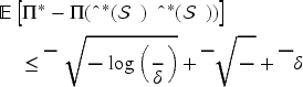
Theorem 1 illustrates that the accuracy of our KM-based estimates for demand-related parameters grows with the data size
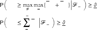
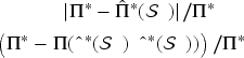
Given any

By Proposition 2, our understanding of the underlying problem would tend to be more accurate when the size of the data set grows. On top of this convergence involving identical replenishment levels, we can still demonstrate a further asymptotic proximity between the optimal values, which are presumably achieved at different replenishment levels. That is, we can show the convergence of
(In-Sample Performance Bound)
Given any number of observations
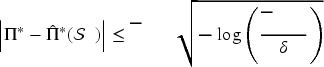
To appreciate Proposition 2 and Corollary 1, imagine that we face a fixed
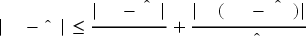
Ultimately, we are interested in the plugging of a solution that is optimal to the data-derived problem back into the true problem. With the two technical results ready, we are now in a position to bound the accuracy of this data-dependent approximation:

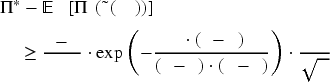
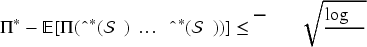
(Regret Bound for the Two-Product Case)
There exists a positive problem-related constant
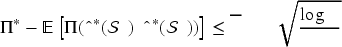
The proof of Theorem 2 relies on the following decomposition:
Indeed, even without multiple products, substitution, or censoring, the regret lower bound is already
When there is one product type, (18) could be simplified into

Suppose
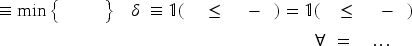
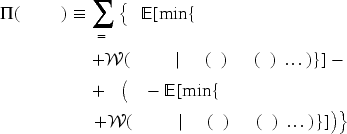
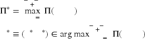
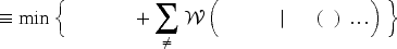
For the profit maximization at a given parameter set in the fashion of (19), a common approach is to exploit the submodularity of the joint profit function (Netessine and Rudi, 2003; Zhang et al., 2021). For our setting, this property reflects diminishing marginal returns achievable by one product’s supply when another product becomes more abundant:
(Submodularity)
The expected profit function
With Theorem 3, the discrete maximization problem involving a general submodular objective function is still NP-hard. Especially, we find our objective
Fortunately, a double greedy heuristic, which optimizes in one dimension while keeping the other dimensions fixed, has turned out to be efficient in approximately maximizing a submodular function in a bounded feasible region; see, for example, Bian et al. (2017) and Zhang et al. (2021). For the current problem involving two discrete decision variables and a rectangular feasible region, the double-greedy idea can be embedded in an algorithm that achieves exact optimality at the expense of a longer running time. This modified double greedy algorithm is also detailed in Appendix B of the E-Companion. It can be shown to terminate at a global maximizer.
Extensions to the Multi-Product Case
We now consider the general model with multi-product substitutions. Although more complicated, the learning procedure here is an extension of its two-product counterpart.
The One-Time Substitution Model
We begin by considering a one-time substitution model where customers attempt substitution among some
Let us define independent random variables
Under unit selling prices
For the current case, the data set when all other products when
We now have the following multi-product counterpart to (13) and (14):
The CCDF’s are then used to compute expectations for the estimations of substitution probabilities in a fashion similar to our earlier approach from (9) to (12). The only differences lie in the definitions of involved coefficients. Corresponding to (9) and (10), we now have
For the profit maximization problem itself, definitions similar to those in (19) and (21) including
The reason for “
Under Assumptions 1
For the static optimization problem under one-time substitution, we also have the multi-product version of Theorem 3 regarding the submodularity of the objective function.
However, the derivation for the multi-product case is considerably more involved than that for its two-product counterpart. We present the details in Appendix E of the E-Companion. To tackle the resulting combinatorial replenishment problem, we adopt a well-established double-greedy heuristic for maximizing submodular functions; see, for example, Bian et al. (2017) and Zhang et al. (2021). In Appendix E of the E-Companion, we describe this heuristic, which iteratively constructs two complementary solutions and merges them through probabilistic updates to achieve a guaranteed constant-factor approximation. We also conduct numerical validations of this heuristic to examine its approximation quality and sensitivity to estimation errors.
We also consider a Markov-chain substitution model, where customers may attempt multiple substitutions until they either meet substitutes or give up on their own volition. Our algorithm would remain effective while achieving a similar regret rate albeit with a less expressive coefficient. Markov-chain choice models as studied by Blanchet et al. (2016) and Şimşek and Topaloglu (2018) were initially not intended for our case with a paucity of data. Nevertheless, we can incorporate into our model the idea of demand shifting according to a homogeneous Markov chain structure.
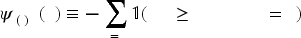
As in the one-time substitution, each product at each block has a base demand, and the substitution probabilities are block-independent. If product
For the multi-product algorithm, recall that (28) estimates base-demand distributions using data in which the starting inventories of all products exceed their respective upper bounds. To brace for the impacts of Markov-chain substitution, we need to modify (29) to

Let


Under the Markov-chain substitution model, there exists a positive problem-related constant such that
Though not presented due to space limitations, we have multi-product counterparts to Proposition 1, Theorem 1, Proposition 2, Corollary 1, and Theorem 2. The multi-product version of the coefficient
Numerical Studies
Our numerical studies use both synthetic and real data. Our real data comes from a central bakery serving multiple stores of a European grocery chain. They can also help to partially verify assumptions.
Synthetic-Data Experiments
We conduct numerical studies to evaluate the performance of our KM-based learning algorithm under different number of products. We also investigate settings in which the true demand upper bounds are unknown. In Appendix D of the E-Companion, we compare our algorithm with the online method of Chen and Chao (2020) and examine the robustness of our approach. In these synthetic-data experiments, block-wise demands within each sixteen-block period follow bounded Poisson distributions. Details are provided in Appendix E of the E-Companion.
Experiments With Different Product Numbers
Here, we evaluate the performance of our algorithm in both two-product and twenty-product settings. Being measured are two relative errors corresponding to Corollary 1 and Theorem 2, respectively:
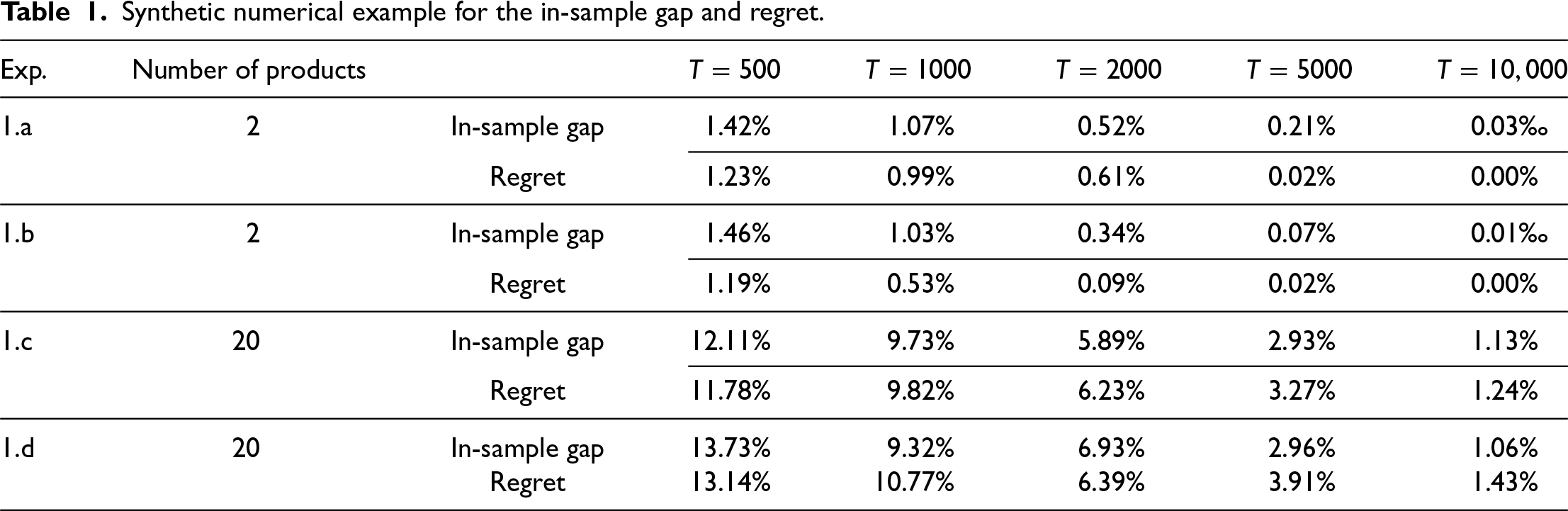
Synthetic numerical example for the in-sample gap and regret.
Synthetic numerical example for the in-sample gap and regret.
From Table 1, we observe that the relative errors decrease steadily across all settings. In the two-product case, our estimates converge rapidly to the ground truth, with the in-sample gap and regret both falling below 1.5% by
When
Moreover, the empirical sensitivities of regret with respect to
We also examine the computational scalability of our methods. The learning procedure for the multi-product case has a polynomial complexity of
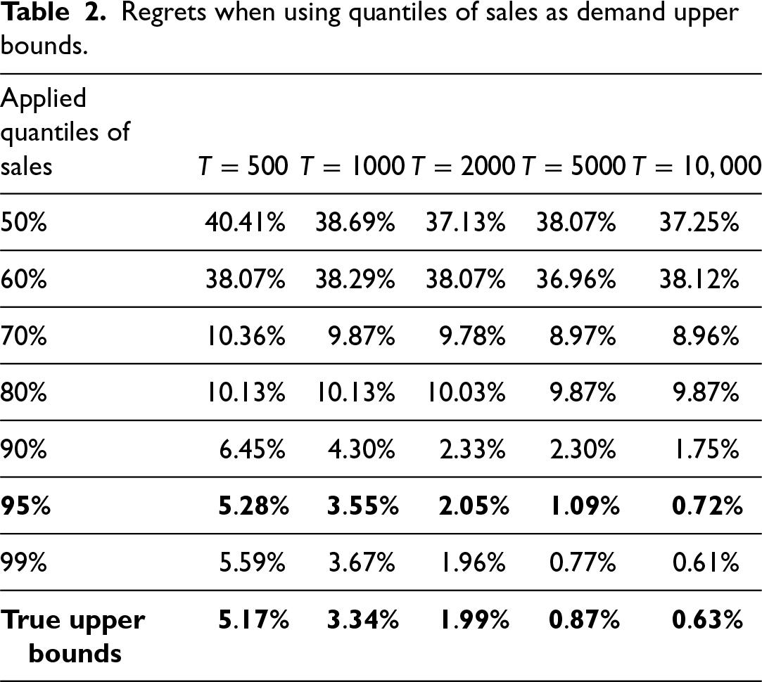
In this experiment, we evaluate the robustness of our KM-based learning algorithm when the true demand upper bounds are not directly observable. Such cases frequently arise in practice because retailers can only observe realized sales, which are often censored by inventory availability. To approximate these unobservable upper bounds, we use different quantiles of the observed sales as proxies for demand upper bounds and then examine how the choices of quantiles affect algorithmic performances.
For each product and block, we take the 50%, 60%, 70%, 80%, 90%, 95%, and 99% quantiles of observed sales as candidate bounds. The algorithm is then executed using these quantiles. The resulting regret levels across different period lengths
Regrets when using quantiles of sales as demand upper bounds.
Regrets when using quantiles of sales as demand upper bounds.
The results in Table 2 indicate that the 95%-quantile of sales provides a strong balance between robustness and accuracy. Lower quantiles (e.g., 60%–80%) tend to underestimate the true upper bounds, leading to premature censoring and thus higher regrets. Conversely, using overly high quantiles, such as 99%, yields minimal additional improvements at the expense of unnecessary computational burdens. The 95%-quantile consistently delivers low regrets, around 1% for
This numerical study is based on a European grocer with hundreds of stores, ranging from small convenience stores in city centers to superstores at suburban locations. We focus on the product category of pre-baked fresh bread, as it dominates store-level waste costs. While representing 40% of baked goods revenue for our selected stores, it represents over 90% of baked goods spoilage, measured in euros.
Each store receives deliveries of pre-baked fresh goods from a local bakery, which does one milk run to multiple stores every day before the stores open. These deliveries are contractually agreed, and do not affect the order quantity decision. On any given day each grocer may request up to 30 fresh pre-baked SKUs, which can be segmented by price (premium or economy), and independently by grain (plain white vs. wholegrain), leading to potential substitutions within each segment.
Store managers at the grocery place order toward the end of each business day, while production at the bakery takes place overnight and all deliveries occur before the stores open. The stock at a grocer is then sold over a business day (
We carry out partial validations of Assumptions 2 and 3; indeed, our seven-product data set would enable those of their multi-product counterparts, Assumptions 2
Assumptions 3 and 3
Our estimates for
We then compare our KM-based learning algorithm against the main benchmarks. There are two popular methods for validating a policy against a data set: In-sample Performance and Out-of-sample Performance.
For In-Sample Performance, we use an entire data set For Out-of-Sample Performance, we split the data set
Methods Considered
We compare the following learning methods to be applied on real data sets. In sample average approximation (SAA) without substitution, we use sample averages of daily demand data while pretending there were no substitutions in order to construct empirical demand distributions. For optimization, we treat the multi-product problem as one where replenishment quantities for different products are set separately. In the KM-based learning approach without substitution, we ignore substitution effects by forcing In the KM-based learning approach with substitution effects, we take substitutions into account in both our learning and optimization.
Experimental Results
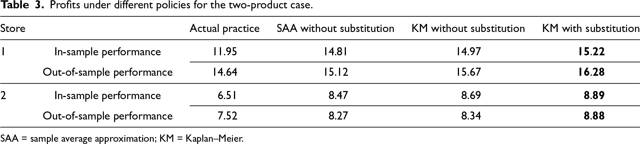
We carry out experiments for two-, three, and seven-product scenarios using real data. For the two-product case, we run experiments for two stores. For Store #1, we have
The resulting profits for the two-product test are listed in Table 3. Besides three columns corresponding to the three methods, we reserve one column for each store’s performance resulting from its actual practice.
Profits under different policies for the two-product case.
Profits under different policies for the two-product case.
SAA = sample average approximation; KM = Kaplan–Meier.
From Table 3, we see that in terms of in-sample performance, our method (KM with substitution) is much better than not only the actual practice but also the with-learning case of SAA for both stores. We also note that KM without substitution, although good enough, is inferior to our method with the substitution effects being considered. On the other hand, we caution that due to de-censoring, the KM estimator describes overall higher demand than the SAA, and adding substitution would mechanically boost the revenue.
For Store #1, the out-of-sample profit is slightly higher than the in-sample one. While the latter is a product of the entire data set, the out-of-sample profit is obtained by optimizing with parameters estimated from the first two-thirds of the data and evaluating the resulting fixed decision under parameters re-estimated from the remaining one-third. In this data set, the realized demand levels during the final one third happen to be higher than those in earlier periods, making this segment more favorable to fixed inventory decisions. A similar pattern is observed for all benchmark approaches. Thus, the higher out-of-sample performance is largely attributable to data characteristics.
We have studied demand learning and replenishment optimization for a multi-product inventory management problem involving both demand censoring and stochastic substitutions. Our efforts have led to a data-driven approach for offline demand learning, the convergence of estimates and attainment of tight regret bounds, an optimization algorithm for the two-product case, and the submodularity of the multi-product case’s objective function. These accomplishments were inspired by a practical retailing problem, to which the literature has not yet provided a satisfactory solution.
There remain promising directions for future research. An efficient solution procedure for the multi-product profit-optimization problem remains elusive. Also, it would be better if our KM-based estimation method relying on only weak censoring indicators could be applied to other inventory problems with complex structures. We have not treated time-varying demand structures. Learning of time-varying parameters has always been a challenging issue; see, for example, Mao et al. (2021) and Chen (2021). New techniques will be required to simultaneously deal with demand censoring and stochastic substitutions.
The block-independence feature of substitution probabilities is furthermore a point that has been exploited by our learning algorithm. In practice, each
Supplemental Material
sj-pdf-1-pao-10.1177_10591478261424592 - Supplemental material for Offline Learning and Optimization for Multi-Product Inventory Management With Stockout-Based Substitution
Supplemental material, sj-pdf-1-pao-10.1177_10591478261424592 for Offline Learning and Optimization for Multi-Product Inventory Management With Stockout-Based Substitution by Yijie Zheng, Youhua (Frank) Chen, Carl Philip T Hedenstierna and Jian Yang in Production and Operations Management
Footnotes
Acknowledgments
The authors thank the Departmental Editor, the Senior Editor, and three anonymous reviewers for valuable comments and suggestions throughout the whole review process.
Declaration of Conflicting Interests
The authors declared no potential conflicts of interest with respect to the research, authorship, and/or publication of this article.
Funding
The authors disclosed receipt of the following financial support for the research, authorship, and/or publication of this article: This work was partially supported by the Hong Kong Research Grants Council (RGC) General Research Fund [Grant CityU 11502122 to Chen YF and Grant PolyU 15511925 to Zheng Y].
How to cite this article
Zheng Y, Chen YF, Hedenstierna CPT and Yang J (2026) Offline Learning and Optimization for Multi-Product Inventory Management With Stockout-Based Substitution. Production and Operations Management XX(XX) 1–20.
References
Supplementary Material
Please find the following supplemental material available below.
For Open Access articles published under a Creative Commons License, all supplemental material carries the same license as the article it is associated with.
For non-Open Access articles published, all supplemental material carries a non-exclusive license, and permission requests for re-use of supplemental material or any part of supplemental material shall be sent directly to the copyright owner as specified in the copyright notice associated with the article.