Linear reactive control for efficient 2D and 3D bipedal walking over rough terrain

Abstract

The kinematics of human walking are largely driven by passive dynamics, but adaptation to varying terrain conditions and responses to perturbations require some form of active control. The basis for this control is often thought to take the form of entrainment between a neural oscillator (i.e., a central pattern generator and/or distributed counterparts) and the mechanical system. Here we use techniques in evolutionary robotics to explore the potential of a purely reactive, linear controller to control bipedal locomotion over rough terrain. In these simulation studies, joint torques are computed as weighted linear sums of sensor states, and the weights are optimized using an evolutionary algorithm. We show that linear reactive control can enable a seven-link 2D biped and a nine-link 3D biped to walk over rough terrain (steps of ∼5% leg length or more in the 2D case). In other words, the simulated walker gradually learns the appropriate weights to achieve stable locomotion. The results indicate that oscillatory neural structures are not necessarily a requirement for robust bipedal walking. The study of purely reactive control through linear feedback may help to reveal some basic control principles of stable walking.

Keywords

Bipedal walking dynamic walking biped reactive control rough terrain evolutionary robotics

1 Introduction

1.1 Background

Animal behavior emerges from dynamic interactions between the nervous system, the body (musculoskeletal system) and the environment (Chiel and Beer, 1997; Chiel, Ting, Ekeberg & Hartmann, 2009). These three factors are interdependent because the body and nervous system co-evolve to produce behavior that is suitable for a particular environment (Sims, 1994).

Bipedal locomotion is an intriguing example of how a complex motor behavior can emerge even in the absence of a nervous system. Tad McGeer showed that bipedal walking is possible in the complete absence of sensing or actuation, a concept he called “passive dynamic walking” (McGeer, 1990). McGeer simulated and constructed bipedal mechanisms with carefully tuned geometric and inertial properties. These bipeds could autonomously walk down a shallow ramp, powered only by gravity. The critical finding of these studies is that the overall process exhibits self-stabilizing attractor dynamics (Strogatz, 2000) that allow the system to fall into a stable limit cycle.

An important limitation on passive dynamic walkers, however, is that they are unable to accommodate environmental disturbances or variations in terrain slope (McGeer, 1990). These limitations underscore the importance of active control (e.g., a nervous system) to robust real-world bipedal locomotor behavior.

The studies of Taga and colleagues offered insight into the neural basis of stable, adaptive walking over unpredictable terrain (Taga, 1995a, 1995b; Taga, Miyake, Yamaguchi, & Shimizu, 1993; Taga, Yamaguchi, & Shimizu, 1991). These authors entrained the mechanics of a 2D seven-link biped to a set of neural oscillators, permitting the biped to traverse uneven terrain and to recover from mechanical perturbations and applied loads to various parts of the body. The authors suggested that “global entrainment” between the neural and musculo-skeletal systems could generate stable and flexible locomotion in an unpredictable environment (Taga, 1995a, 1995b).

Although these studies demonstrated that neural oscillator-based control is sufficient for some aspects of gait adaptation, they did not demonstrate that it is necessary. In the present work we use simulations to investigate the potential for a purely “linear reactive” controller to enable stable and flexible locomotion over rugged terrain. By reactive we mean that there is a fixed mapping between sensor input and motor output. By linear, we mean that the mapping is a weighted sum of the sensor inputs. The existence of such a control scheme would call into question the fundamental necessity of coupling between a neural oscillator and the mechanical system for bipedal walking.

The present work was originally motivated by “Braitenberg Vehicles,” which demonstrate that complex behaviors can emerge from simple reactive control laws (Braitenberg, 1984; Mondada and Floreano, 1995; Eiben and Smith, 2003). In a recent paper, we used control laws similar to those used by Braitenberg to simulate stable and efficient locomotion of a five-link biped robot (Solomon, Wisse, & Hartmann, 2010). The five-link biped was able to walk over unpredictable terrain, with slopes varying between 2° and 7°, and step-downs varying between 0 and 25% leg length (Solomon et al., 2010). However, this five-link biped did not have feet and was only trained to walk downhill.

The present study extends these previous results to implement linear reactive control in simulations of both a 2D seven-link biped (in which feet and ankles have been added to the previous model) and a 3D nine-link biped (in which hips and another spatial dimension have been added). Weights are tuned with an evolutionary algorithm (EA) to achieve efficient and stable walking over rough terrain (step-to-step standard deviations in terrain height of 5.4% and 2.0% of the leg length for the 2D and 3D walkers, respectively) with a sparsely interconnected linear reactive controller. The work suggests that “physical entrainment” involving only the dynamic interaction between body and environment is sufficient to enable adaptive locomotion control; internal neural dynamics, i.e., global entrainment, is found to be unnecessary.

1.2 Related work

The scope of research related to bipedal locomotion control is vast. Here we briefly review some relevant studies that fall under the bipedal “dynamic walking” paradigm, as opposed to the popular zero moment point control (Vukobratović and Borovac, 2004). Following McGeer’s pioneering work, several studies focused on issues of energy efficiency and stability in passive dynamic walking (Garcia, Chatterjee, Ruina, & Coleman, 1998). Work by Kuo (2002) demonstrated methods to add actuation and feedback control to enable stable walking over level ground. Collins and Ruina (2005) implemented a variation of ankle push-off actuation studied by Kuo on a 3D bipedal robot, which exhibited energy efficiency on par with humans. Hobbelen and Wisse developed several simple and effective control strategies, including swing leg retraction near the end of a step (Hobbelen and Wisse, 2008c), local stance ankle control and ankle push-off modulation (Hobbelen and Wisse, 2008a), modulation of walking speed (Hobbelen and Wisse, 2008b), and a linear, lateral foot placement strategy (Hobbelen and Wisse, 2009). All were successfully implemented on the planarized (2D) robot “Meta” and/or the fully 3D robot “Flame” (Hobbelen, de Boer & Wisse, 2008). Chevallereau et al. (2003) analytically derive a controller based on the concepts of “hybrid zero dynamics” and “virtual constraints,” achieving successful implementation on the 2D robot “RABBIT”. Byl and Tedrake (2009) apply an approximate optimal control method with one-step planning to a compass gait model, enabling it to traverse rough terrain.

Particularly relevant to the present study is research involving simple reflex-based models. Ono, Takahashi and Shimada (2001) developed a control strategy based on setting the hip torque proportional to knee angle and linearly damping the knee joint, and successfully instantiated it on a 2D biped robot on a shallow slope. Manoonpong, Geng, Kulvicius, Porr, and Wörgötter (2007) designed a neural network control architecture based on the design principle of nested sensorimotor loops and applied it to a 2D robot, “RunBot,” demonstrating fast and efficient walking performance with the ability to adapt to varying terrain slopes. Geyer and Herr (2010) apply a muscle reflex model based on positive force and length feedback schemes to a 2D, seven-link model, exhibiting angle and torque activation patterns qualitatively similar to humans. Most similar to the present study, Paul (2005) used feed-forward neural networks to compute desired joint angles for proportional-derivative (PD) control of a simulated 3D biped over level terrain, tuning the weights with an EA. We recently applied a controller similar to that studied here to a 2D five-link model (Solomon et al., 2010). It was able to reject large step-down disturbances and adapt to changing slopes, but, critically, did not incorporate feet and was only trained on downhill slopes.

2 Methods

The present work uses both 2D and 3D biped models. Most of the results presented here focus on the 2D model, as its faster simulation speed allowed a larger number of EA runs. The 2D equations of motion were derived using the TMT method (Wisse and Schwab, 2005) and solved by Euler integration, while the 3D model was developed using the Open Dynamics Engine (version 0.11.1) as a simulation environment (Smith, 2009). We used anthropomorphic dynamic parameters for the 2D model (Winter, 1991) to allow direct comparison with the kinematics and actuation torques measured in human locomotion, and the 3D model’s parameters were based on the Delft University of Technology’s prototype “Flame” to test the controller’s potential performance on a plausible real-world testbed (Locascio, Solomon & Hartmann, in press).

2.1 Two- and three-dimensional biped models

The 2D model consisted of seven links: an upper body, two thighs, two shanks, and two feet, as shown in Figure 1a. Parameter values for the 2D model are provided in (Wisse, 2008; Locascio et al. in press; Table 1), and are based on typical values for a 70-kg, 1.75-m tall human (Winter, 1991). Note that the center of mass distance for each segment is measured relative to its “parent” joint (e.g., the hip joint for the thigh segment). Also, three length values are provided for the foot; these correspond to heel-to-toe length, heel-to-instep length, and instep-to-ankle length, where “instep” refers to the point on the bottom of the foot directly below the ankle when the foot is flat on the ground. The foot center of mass resides at the geometric center of the foot. Geometric and inertial parameter values for the 3D model are provided in the FLAME documentation (Wisse, 2008; Locascio et al., in press).

Figure 1.

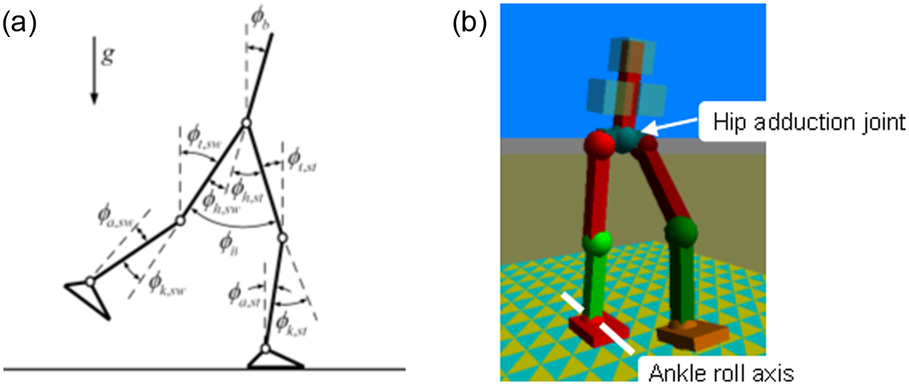
The 2D seven-link and 3D nine-link biped models used in this study. (a) The 2D model incorporates a total of seven degrees of freedom. (b) The 3D walking model is a straightforward extension of the 2D model. In addition to the features of the 2D model, the ankles have a “passively” actuated degree of freedom (simulated springs, including damping), and two links were added to allow symmetric hip adduction.

Table 1.

Parameter values for the seven-link model

	body	thigh	shank	foot
Mass, m [kg]	47.5	7.00	3.26	1.02
Length, l [m]	−	0.430	0.430	0.210, 0.052, 0.068
Center of mass, c [m]	0.316	0.186	0.186	0.057
Moment of inertia, I [kg·m²]	2.966	0.134	0.055	0.005

The body length is not provided because it plays no role in the biped’s dynamics (i.e., the position of the center of mass and the moment of inertia are present in the equations of motion, but not the full body length). The three foot lengths refer to heel-to-toe length, heel-to-instep length, and instep-to-ankle length, respectively.

The 3D model, shown in Figure 1b, includes the same seven links as the 2D model, plus two hip links, used to introduce a pelvic width into the model and to allow independent hip adduction/abduction (hereafter simply “adduction” for brevity) and hip flexion/extension. These two links are mechanically constrained (consistent with the real Flame) such that the left and right legs cannot adduct independently, but must always have the same angle relative to the torso. The imposition of this symmetry simplifies the model, while still allowing sufficient step-width control. There is an additional degree of freedom in the ankles, allowing them to “roll” about the axis indicated in Figure 1b. This degree of freedom is un-actuated, but is under the influence of passive torsional springs. Thus, only a single additional actuator (hip adduction) was added to the 3D model. Both the 2D and the 3D models include encoder sensors that measure the angle and velocity of each joint, an inertial sensor to measure the upper body angle and velocity with respect to gravity, and a binary contact sensor at the heel and toe of each foot. Each of the six joints in the 2D model has a torque-controlled actuator, while the 3D model also has one additional actuator for hip abduction/adduction, and corresponding position and velocity sensors at that joint.

The equations of motion for the 2D model were implemented in C++ for fast execution. The first-order Euler method was used to integrate the equations of motion, with a time step of 0.0002 s. A more accurate solver, such as fourth-order Runge–Kutta could have been used, but would have run at a quarter of the speed, and was found to negligibly affect the behavior of the model. The 3D model was simulated in the Open Dynamics Engine using a 0.001-s time step, congruent with the time step used in Flame’s real-time operating system.

The following notation is used throughout this paper to describe the degrees of freedom of the 2D and 3D models. The 2D model has seven degrees of freedom: one defines the “upper-body” angle with respect to gravity $ϕ_{b}$ , two define the “hip” angles between the upper-body and thigh segments $ϕ_{h, st}$ and $ϕ_{h, sw}$ , two define the “knee” angles between the thigh and shank segments $ϕ_{k, st}$ and $ϕ_{k, sw}$ , and two define the “ankle” angles between the shank and foot segments $ϕ_{a, st}$ and $ϕ_{a, sw}$ . The abbreviations “st” and “sw” indicate whether the angle is associated with the “stance” leg or “swing” leg, respectively. Also note that absolute (with respect to gravity) “thigh” segment angles $ϕ_{t, st}$ and $ϕ_{t, sw}$ and the “inter-leg” angle $ϕ_{il}$ have been defined because they are used for control purposes. The 3D model adds theactuated hip adduction angle $ϕ_{ad}$ , the upper-body yaw and roll angles $ϕ_{b, yaw}$ and $ϕ_{b, roll}$ , and the unactuated ankle roll angles $ϕ_{r, st}$ and $ϕ_{r, sw}$ .

In both the 2D and the 3D models, joint angle limits were enforced using “soft” constraints, effectively by implementing stiff PD controllers with the gains manually tuned to produce good qualitative behavior of the model (typically <1° overshoot). Although enforcement of all constraints occurred frequently in the early stages of controller evolution, only the knee hyperextension constraint was regularly enacted during normal locomotion in the 2D model. In other words, successful walkers gradually learned to operate in the absence of the constraints on joint angle limits, except for knee hyperextension. Table 2 provides the joint angle constraints and associated PD gains for the 2D model. The 3D model shares joint angle constraints with the Flame prototype (Hobbelen et al., 2008).

Table 2.

Joint angle limits and the proportional-derivative (PD) gains used to enforce them

	Min. φ [rad]	Max. φ [rad]	P gain $[N \cdot m / rad]$	D gain $[N \cdot m \cdot s / rad]$
Hip	$- π / 3$	$π / 3$	100	5
Knee	$- π / 2$	0	300	15
Ankle	$- π / 4$	$π / 4$	5	0.25

An important note is that we chose to control the upper-body $ϕ_{b}$ and inter-leg $ϕ_{il}$ angles instead of directly controlling the hip angles $ϕ_{h, st}$ and $ϕ_{h, sw}$ in both the 2D and 3D models. As will be shown, this choice of actuation allows PD control of walking with fixed set points, which is not possible using only the hip angles, as they do not take into account the angle of the upper body with respect to gravity.

2.2 Terrain models

Care was taken to devise simple methods to generate unpredictable, rough terrain with features determined by a few intuitive parameters. The 2D terrain morphology is numerically defined by a series of $(x, y)$ points, regularly spaced in the x-direction in 0.1-m increments. The vertical spacing between adjacent points is computed by generating a traditional “random walk” sequence, and then smoothing it using a 5-point moving average. The vertical step size was chosen to be 0.0176 m, such that the slope of the terrain was limited to the range [−10°, 10°], and the effective step-to-step standard deviation in terrain height was typically ∼5.4% leg length (including the foot), nicely following a normal distribution. A similar technique was used for the 3D terrain, although this technique was slightly more complicated and is described in Appendix A. Two different sets of 3D terrains were used during evolution, one with effective step-to-step standard deviations of ∼0.36% leg-length, and one with linearly increasing standard deviations up to ∼3.6% leg-length. The advantages of this method are that it is simple, efficient, automatically puts an upper limit on the slope magnitude, and stochastically generates empirically interesting features, including relatively flat regions of various slopes, abrupt changes in slope, and higher frequency bumpy regions. Typical samples of the 2D and 3D terrains used in this study are shown in Figure 2.

Figure 2.

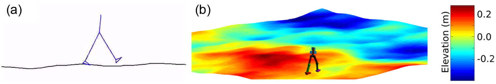
Examples of typical 2D and 3D terrain.

2.3 Models of ground contact

The foot-ground contact of the 2D model was modeled using soft constraints, as described in Haavisto and Hyötyniemi (2004). A stiff spring (k_p,terrain=50,000 N/m) and damper (k_d,terrain=2500 N·s/m) push on a heel or toe whenever penetration with the ground is detected through linear interpolation between the (x,y) terrain points. A traditional Coulomb friction model is also implemented, such that the maximum tangential force $F_{t}$ is proportional to the normal force $F_{n}$ through the static friction coefficient $μ_{s} = 1.2$ . Hence, whenever the spring-damper tangential force exceeds the maximum normal force $F_{t, max} = μ_{s} F_{n}$ , the applied tangential force becomes $F_{t} = μ_{k} F_{n}$ , where $μ_{k} = 0.6$ is the kinetic friction coefficient, and the heel or toe begins to slide.

In the 3D model, collisions were detected between the model and the ground heightfield using the OPCODE collision detection engine (Terdiman, 2003). When collisions between the feet and the ground were detected, temporary constraints were placed at those positions. ODE’s “error-reduction” and “constraint-force-mixing” parameters for those constraints were set in order to produce spring and damper coefficients equivalent to the 2D model.

2.4 Control model

The control approach used here deviates significantly from traditional control theory; the overall methodology more closely resembles work in the field of artificial neural networks (ANNs), and hence terminology from that field will be used (Bishop, 1996). As schematized in Figure 3a, the output of each actuator is computed from a weighted linear sum of sensor states and a bias. Alternatively, the output of the network can be interpreted as a desired angle, and the actuator torque is then calculated via PD control using this as a reference (Figure 3b). Equivalent weight sets can be found for the two forms such that they produce identical results. This “linear reactive” control architecture was used for both the 2D and the 3D models, which we now describe in detail.

Figure 3.

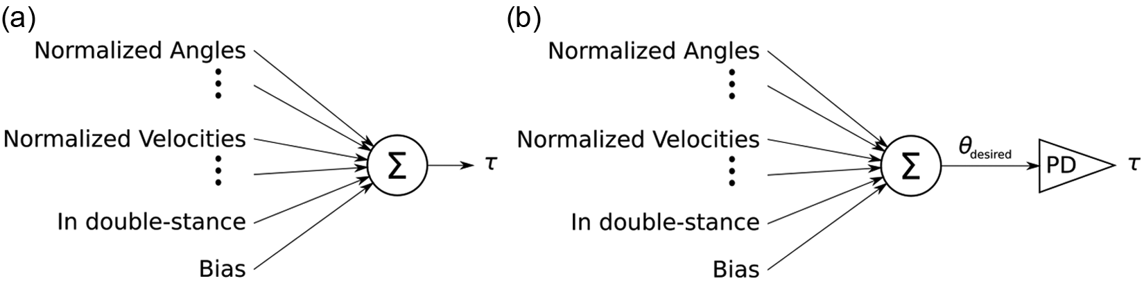
The controller architecture, in which torques are computed as a weighted sum of sensor inputs. Here, each arrow connecting the input to the summing block is weighted by some value, which will be tuned by an evolutionary algorithm (EA). (a) Direct torque output. (b) Desired angle output, in which torque is computed via PD control. In this study, zero was always used as the reference velocity in order to apply damping to the system.

The 2D biped model has six actuators: stance/swing ankle, stance/swing knee, and stance/swing hip. In the “fully connected” configuration, each actuator’s output is computed from 16 inputs. The sixteen network inputs include seven angles ( $ϕ_{b}$ , $ϕ_{t, st}$ , $ϕ_{il}$ , $ϕ_{k, st}$ , $ϕ_{k, sw}$ , $ϕ_{a, st}$ , $ϕ_{a, sw}$ ), their derivatives, the variable in_double_stance (a Boolean that indicates whether both feet are in ground contact), and a bias. A bias term is standard in machine learning algorithms as a way to provide a constant, non-zero input to a function (e.g., the intercept term of a linear regression). The network input vector thus accounts for a full state description of the robot except for its absolute spatial position and velocity, which are not necessary for control of walking. Inputs $ϕ_{b}$ , $ϕ_{k, st}$ , $ϕ_{k, sw}$ , $ϕ_{a, st}$ , $ϕ_{a, sw}$ are direct sensor (inertial and encoder) states, and stance thigh $ϕ_{t, st}$ angle and inter-leg angle $ϕ_{il}$ are computed from sensor states as follows:

ϕ_{t, st} = ϕ_{h, st} - ϕ_{b}

(1)

ϕ_{il} = ϕ_{h, sw} - ϕ_{h, st}

(2)

The 3D biped model has seven actuators: the same six as in 2D, plus hip adduction. In the “fully connected” 3D configuration—which was never used in the present study—the output of each of the seven actuators is computed from all 28 inputs, for a total of 196 weights. Each of the seven actuator networks consisted of 25 state variables, plus the P and D gains for the “angle output” configuration, and one constant bias term. The sensor inputs include the same 16 from the 2D model, plus the roll and yaw of the torso, the hip adduction angle, the stance and swing ankle roll values, and the time derivatives of these five values. This highlights an important benefit of the linear reactive control framework, namely, the simplicity of scaling. The transition from a 2D controller to 3D required only two changes: addition of a network to control the one additional actuator, and addition of these 3D-specific inputs.

A complication arises in the interpretation of the torso roll and yaw angles used as inputs to the network. The signs of these values must be adjusted to be stance-foot dependent. This way, a roll sensor value indicating that the torso is leaning left will result in a different network input (and therefore, a different control action) depending on which is the stance foot. This is implemented simply by multiplying the roll, the yaw, and their velocities by −1 if the left foot is the stance foot. The choice of left or right in this instance is arbitrary, as the signs of the connection weights will be set accordingly by the EA.

Simulations of both 2D and 3D models proceed as follows: at each time step, the sensor state of the model is measured. An affine transformation is used to shift and scale all values to a range of roughly [−1, +1]. A weighted sum of normalized sensor inputs is computed as in Figure 3, and for the 2D model the output is used directly as a torque (as in Figure 3a), while for 3D model it was used indirectly as a desired joint angle for PD control (as in Figure 3b). In practice, either interpretation of the sensor output can be used for both the 2D and 3D case. Further details can be found in Appendix B.

An important detail is identifying which leg is “stance” and which is “swing,” as this determines which network controls which actuator at any given time. The two legs are trivial to identify during the swing phase (one contact sensor is high, the other is low). During the double-stance phase, we defined the “trailing” leg (the leg whose ankle is more caudal in the direction of travel) as the stance leg. This was necessary to ensure that the stance leg had the higher torques required for push-off, and that the inter-leg angle remained relatively unchanged during push-off. A flight phase was not permitted (i.e., considered a “fall” during weight optimization).

2.5 Variations on the control model

Figure 3 and Section 2.4 present the “fully interconnected” version of the 2D and 3D control architecture, in which actuator output is calculated as a linear sum of all of the inputs. The present work focuses on the following four variations of this “linear reactive” control framework in the 2D model, and then explores the use of one variation in the 3D model. Note that the networks vary only with respect to the number and identity of the input connections.

2.5.1 Local proportional-derivative (LPD) configuration (three inputs/actuator)

The LPD configuration makes use of only three inputs per actuator. In the case of direct torque output, the angle and angular velocity of the associated joint and a bias are used to compute the motor torque, which is equivalent to a PD controller with a fixed set point. For example, the swing leg’s knee torque would only be based on a weighted sum of the swing leg knee angle, velocity, and a constant offset. It would not be surprising if such a minimalistic control policy were completely insufficient for generating stable locomotion over rough terrain, but it will be shown that impressively stable and fluid walking behavior can be achieved.

2.5.2 Fully interconnected linear (FIL) configuration (16 inputs/actuator)

The FIL configuration tests the capacity of using all sensor states as inputs to all networks of the model to improve upon the efficiency and stability of LPD control. Intuitively, more sensor information should result in better control.

2.5.3 Sparsely interconnected linear (SIL) networks (between one and 16 inputs/actuator)

To generate the SIL networks for the 2D model, connections of the FIL networks are slowly pruned away until performance starts to decline. This addresses the question of which non-local connections are actually conferring significant performance benefit, and in doing so, may provide insights relevant to controlling bipedal robots as well as insights into the nature of human locomotion. The smaller search spaces compared to the FIL networks should also reduce the optimization time.

An SIL network identified using the 2D data was used for the 3D walking trials. A hip adduction actuator network had to be added, for which the inputs were manually chosen based on their intuitive relevance for lateral control: the torso roll and yaw angles and velocities, as well as the stance ankle (plantarflexion/dorsiflexion) angle and velocity. The values of the weights were then optimized from scratch (i.e., were not biased using the values found from optimizing the 2D model).

2.5.4 Reduced, sparsely interconnected linear (RSIL) networks (between one and 16 inputs/actuator)

Finally, the connections most frequently remaining after pruning SIL networks were used to create “reduced” SIL networks. The methods used to achieve the “reduction” will be explained more fully in Results. The goal in developing RSIL networks was to determine the performance achievable when using a minimal set of connections.

2.6 Gait initiation and gait termination

We used two different methods to initiate stable walking in the simulations. For the 2D simulations, we extended the linear reactive controller of Section 2.4 to enable gait initiation behavior starting from a static stance state. Specifically, we defined an additional set of network weights, the “initiation weights” ${\bar{W}}_{init}$ , wherein each weight is paired with a corresponding one from the locomotion controller set of “walking weights” ${\bar{W}}_{walk}$ . Gait initiation begins with the biped in a static state, with its legs side-by-side (although any statically stable configuration is permissible). Then, from t=0 seconds to t=t_init seconds, the weights linearly scale with time from ${\bar{W}}_{init}$ to ${\bar{W}}_{walk}$ as follows:

\begin{matrix} W_{net} (n, i) = \\ {\begin{matrix} (1 - \frac{t}{t_init}) \cdot W_{init} (n, i) + \frac{t}{t_init} \cdot W_{walk} (n, i) t < & t_init \\ W_{walk} (n, i) & t \geq t_init \end{matrix} \end{matrix} .

(3)

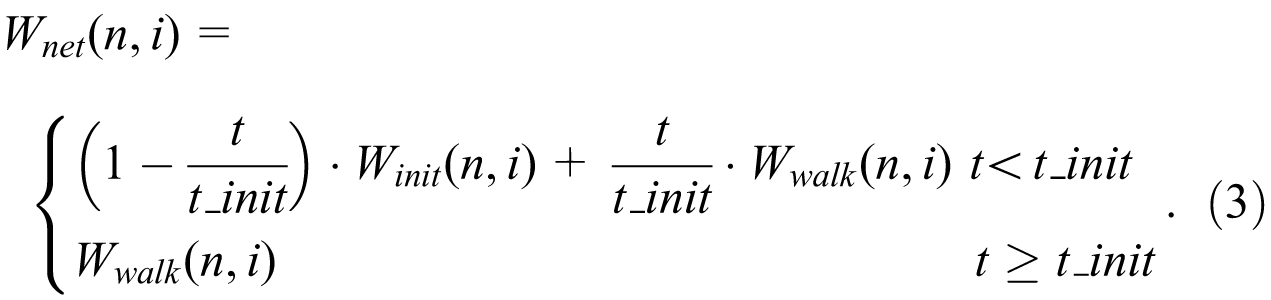
As the network weights linearly scale from the initiation weights to the walking weights, the desired behavior is simply for the biped to take a smooth, stable step forward. Note that a nearly identical procedure can also be used for gait termination, and indeed was found to be effective (results not shown).

The lack of lateral stability in 3D simulations adds considerable complexity to the control of gait initiation; hence we could not obtain reliable gait initiation with Equation 3. Therefore, 3D walking was initiated using a fixed initial state amenable to walking, in which the swing foot was already in the air and the inter-leg angle was increasing. This approach had the disadvantage of restricting the range of possible weight sets to those that are “compatible” with the initial conditions, but did not prevent us from successfully evolving controllers.

2.7 Evolutionary optimization

Because of the large number of parameters that need to be tuned as well as the stochasticity of the terrain model, the majority of standard numerical optimization approaches are poorly suited for the current problem. However, one family of optimization methods, EAs, clearly stand out in these respects. EAs are stochastic, population-based metaheuristic optimization procedures inspired by principles of neo-Darwinian evolution (selection, crossover, and mutation; Eiben and Smith, 2003). They generally scale well with problem size, can handle stochasticity in the fitness function, and have proven effective in optimizing control parameters for numerous locomotion studies (Hasegawa, Arakawa, & Fukuda, 2000; Reil and Husbands, 2002; Vaughan, Di Paolo, & Harvey, 2004). Of the four main historical branches of EAs—genetic algorithms, evolution strategies, evolutionary programming, and genetic programming—the algorithm used here is most similar to evolution strategies, although there are some customizations, as will be explained.

2.7.1 Evolutionary parameters

Having defined the control framework, the remaining critical component to enable successful walking was the optimization of control parameters. We used an EA to optimize the connection weights of all actuator networks. One cannot expect to truly optimize such a large set of parameters for the type of control problem investigated here. We therefore use the word “optimization” only in the sense that it describes the attempt to maximize (or minimize) some quantity, perhaps finding a local optimum.

As described in Section 2.6, the control parameters for 2D walking consist of six sets of gait initiation weights ${\bar{W}}_{init}$ , six sets of walking weights ${\bar{W}}_{walk}$ , and the t_init parameter. Additionally, six evolutionary “learning rate” parameters $\bar{α}$ (one for each network) are included to improve the optimization.

In the 2D LPD network mapping there are three weights associated with each of the six actuators for both the initiation weights $({\bar{W}}_{init})$ and walking weights $({\bar{W}}_{walk})$ , along with the six learning rates, yielding a total of $6 \cdot 3 + 6 \cdot 3 + 6 + 1 = 43$ parameters. The 2D FIL mapping has 16 weights per set, yielding $6 \cdot 16 + 6 \cdot 16 + 6 + 1 = 199$ parameters, and for the 2D SIL and RSIL frameworks the number of weights can vary.

The learning rate parameters $\bar{α}$ are used in the 2D trials to automatically scale the nominal mutation sizes of each of the networks. They serve an analogous function to the “strategy” parameters in the evolution strategies algorithm (Eiben and Smith, 2003). The general idea is that choosing proper mutation sizes can be critical to ensure optimization, given that certain parameters or groups of parameters may require bigger or smaller mutations. For example, the stance ankle controller will generally output larger torques than the swing ankle controller, and hence larger changes in torque output (i.e., bigger mutations) are required to significantly affect the resulting behaviors.

Moreover, optimization results may be improved if mutation sizes are allowed to change during the course of evolution, regardless of their initial values. For example, the initial mutation sizes might need to be large at the start of an evolutionary run to prevent falling into a local minimum, but smaller at the end of the run to allow refinement of the controller. These issues are addressed by defining learning rates for each of the networks, and having evolutionary pressures adapt them alongside the control parameters for effective optimization. The 2D model was used to provide initial estimates of the evolutionary parameters, which were then implemented in the 3D model with minor changes.

2.7.2 Fitness function

We used a fitness function that placed strong emphasis on both stability and efficiency. Fitness was defined as “the distance traveled before falling down or expending a fixed amount of joint torque cost.” In this function, distance traveled is the distance the biped has moved in the x-direction, measured at the hip, and “joint torque cost” is a concept similar to mechanical energy expenditure (Srinivasan, Westervelt & Hansen, 2009).

The joint torque cost is computed using

C_{τ} = \sum_{n = 1}^{N} \int_{0}^{T} | τ_{n} | \cdot d t

(4)

where T is the total time elapsed since the start of the trial and $τ_{n}$ is the torque of the motor for the nth network. Torque cost is used in place of mechanical energy for a number of reasons. First, joint torque cost may be a better reflection of true metabolic expenditure in humans, as well as a better reflection of battery power expenditure in robots (as will be explained in Section 4.3). Also, integrating the product of torque and angular velocity to compute energy has the effect of producing stiff walking behaviors in which joint velocities are kept very low, resulting in small mechanical energy expenditures.

With this fitness function, stability is required for high fitness because falling down will lead to a short distance traveled, and therefore, low fitness. Efficiency is required for high fitness because the more quickly the fixed amount of joint torque cost is expended, the shorter the distance traveled, and the lower the fitness. Thus, maximizing fitness is tantamount to simultaneously optimizing both stability and efficiency.

2.7.3 Evolution procedure

In the 2D model, the EA starts out by generating an initial population (generation g=0) of 150 genotypes (sets of weights) for the LPD network configuration. The walking weights ${\bar{W}}_{walk}$ of the initial population were manually tuned to be equivalent to PD controllers with effective gains of ${\bar{k}}_{p} = [300, 100, 300, 10, 300, 20]$ N·m, ${\bar{k}}_{d} = [15, 0, 15, 0, 0, 1]$ N·m·s, and the set points uniformly distributed between −1 and +1 radians. The gait initiation weights ${\bar{W}}_{init}$ were generated uniformly in the range of [−1, 1], t_init uniformly in the range [0, 2] seconds, and the learning rates were biased around unity. During each EA run, the values of all weight parameters were unconstrained, while the learning rates were constrained to be greater than zero and t_init was constrained to [0, 2]. Each generation involved the following steps:

Selection—The population is ranked by fitness, and those in the top 20% are chosen as parents for the subsequent generation (so-called $(μ, λ)$ selection; Eiben and Smith, 2003).

Crossover and mutation—The best parent is directly copied (elitism). The remaining 149 offspring are generated by either crossover between two random parents (25% probability), mutation of a random parent (25% probability), or by crossover between two random parents followed by mutation (50% probability). The crossover operation is “discrete,” meaning that each parameter is randomly chosen from either parent. The mutation operator simply adds a normally distributed random vector to the genotype vector, with the standard deviations set to 0.05 for the LPD configuration, and 0.005 for the FIL and SIL configurations. Smaller mutations are used in the latter cases due to the larger number of weights.

Fitness evaluation—The fitness of each member of the population is evaluated, with $C_{τ} = 3000$ N·m·s for the LPD runs, and $C_{τ} = 1000$ N·m·s for the FIL and SIL runs. The LPD runs were given three times as much joint torque cost in order to compensate for the reduced efficiency of the LPD controllers. The terrain is randomly regenerated for each fitness evaluation.

Repeat or stop—If the final generation g is reached (g=500 for LPD run and g=3000 for the FIL run) or other stopping condition is met (for the SIL runs), then stop. Otherwise, return to step 1.

In the 3D trials, the procedure remained nearly the same. As previously mentioned, the gait initiation procedure is removed. Elitism was also not used for the 3D optimizations. LPD walkers were uniformly less successful in 3D, as they lacked any mechanism for dynamic step-width control. As a result, only the SIL configuration described in Section 2.5.3 was used for 3D. One set of SIL connections from a 2D run was used for the six actuators shared between 2D and 3D. Connections likely to be important for the hip adduction actuator were chosen for that network: torso roll, torso yaw, hip adduction angle, stance ankle (plantarflexion/dorsiflexion) angle, and the velocity of each of these. All individuals were given $C_{τ} = 1000$ N·m·s of torque cost. The crossover and mutation probabilities were the same, and the mutation standard deviation was the same as in the 2D FIL runs.

Because of the stochastic nature of the fitness evaluations, it is probable that the fittest individual of the final generation is actually not the fittest individual of the overall run. To select the fittest overall individual, the elite individuals of the last 50 generations were evaluated on twenty new terrains. The individual with the highest average fitness was declared the winner. The winner was then evaluated on 1000 newly generated terrains to accurately measure its fitness.

2.7.4 Bootstrapping

Optimizing the FIL weights in 2D followed a procedure very similar to that of the LPD weights in 2D, except for how the initial population was generated. Several attempts were made at evolving a FIL controller by generating the initial weights according to various random distributions, but walking behaviors did not even begin to evolve. This is a common phenomenon in the field of evolutionary robotics called the “bootstrap problem,” wherein completely random parameters lead to controllers that all perform so poorly that learning cannot get started (or the population quickly falls into a highly suboptimal local minimum) (Nolfi and Floreano, 2004).

To address this issue, each winner of the LPD tournaments was used as a bias around which the initial populations of FIL weights were centered (with a standard deviation of 0.05 on all weights to add diversity). Thus, the initial FIL populations started out with successfully walking individuals, and evolution could incrementally ascend gradients in fitness space for gradual improvement. The EA proceeded in the same manner as with the LPD weights, but using smaller mutation sizes of 0.005 in all generations after the first to allow thorough optimization of the additional weights. A total of 50 runs were conducted, and final tournaments were again held to determine the best-performing individual of each run.

The 3D SIL trials also required bootstrapping. A set of hand-chosen LPD weights were incorporated into the parents of generation 0, and all other connection weights were set to zero. These weights encoded elementary walking behavior such as increasing inter-leg angle and locking of the stance knee. Evolution proceeded successfully from this point.

2.7.5 Identifying the important links

Additional analysis was performed to determine which of the network links played important roles in the controller. For example, it seems likely that the network that controls the stance knee torque would not benefit significantly from the input link associated with the swing ankle velocity, but how should this be determined? Our analysis involved continuing each of the 50 original 2D FIL runs, but now pruning a random link (excluding the link associated with the local angle, angular velocity, and the bias) from each member of the population (except the elite) every 10th generation, starting at generation 3001. When the median fitness of the 10 most recent elite individuals became less than 90% that of the median fitness of the elite from the final 50 generations of the original run (generations 2951 to 3000), the removal of links was halted. In other words, links were gradually removed until doing so started to have a significant impact on the fitness of the population. The EA was then run for an additional 200 generations without further pruning to optimize the weights in the context of the reduced but consistent set of connections. Finally, tournaments were held to identify and evaluate the best performing SIL controller resulting from each run. This process produced the SIL configurations.

In order to consolidate the results of the 50 pruning runs and identify which connections played the most important roles, we conducted a threshold analysis. Any connection that remained for at least 80% of the pruning runs was kept, and the rest were removed. The 80% threshold was chosen through trial and error, such that fitness did not degrade significantly compared to the previously evolved SIL controllers, while attempting to remove as many connections as possible. The connection weights of the RSIL controller were then evolved from scratch for 10 runs (while again, as with the FIL controller, biasing the LPD weights) to evaluate its performance.

3 Results

As described in Section 2.5, we focus on four variations of the controller shown in Figure 3: “local proportional-derivative” (LPD); “fully interconnected linear” (FIL); “sparsely interconnected linear” (SIL); and “reduced, sparsely interconnected linear” (RSIL).

These results are first explored in two dimensions (Sections 3.1–3.4) in order to analyze the general principles. Building on the results from the 2D simulations, we then evolved controllers for the 3D model that could also navigate rough terrain under linear reactive control (Section 3.5).

3.1 EA results for 2D walkers

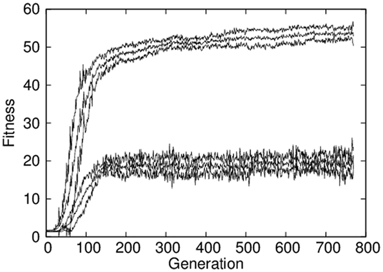
We evolved linear reactive controllers for 2D bipedal walking over terrain with characteristics described in Section 2.2. Successful walking for one particular FIL controller can be seen in the video in Supplemental Online Materials. FIL controllers were found with mechanical cost of transport $C_{mt}$ as low as 0.033 (0.044 average) and fall percentage as low as 2.0% (12.8% average), and similar results were obtained for the SIL and RSIL configurations, as shown below.

The EA results for the 2D model are shown in Figure 4a, which plots fitness as a function of generation, averaged over 50 runs. The first 500 generations are for the LPD learning phase, the next 3000 are for the FIL learning phase, followed by 564 generations for the pruning phase, and finally 200 generations for post-pruning optimization. The pruning phase actually lasted a different number of generations for each run—between 353 and 854—depending on when fitness started to fall significantly. Averaging this portion of the plot involved scaling each set of data from the pruning phase to the average length of 564 generations. In Figure 4a, fitness values for the LPD phase were scaled by a third, because those controllers were allotted three times as much joint torque cost to compensate for their reduced efficiency.

Figure 4.

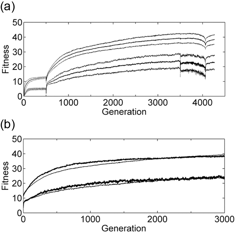
(a) Results of the evolutionary algorithm (EA) optimization, averaged over the 50 runs. The upper three curves represent the maximum fitness±the standard deviation of maximum fitness values, and the bottom three curves represent the mean fitness±the standard deviation of mean fitness values. (b) Results of the 10 reduced, sparsely interconnected linear (RSIL) runs (thick lines) and 50 fully interconnected linear (FIL) runs (thin lines). The upper curves represent the maximum fitness, and the lower curves represent the mean fitness.

Figure 4a shows that fitness values started to increase steadily at the beginning of the FIL phase, due to the increased efficiency afforded by the non-local connections. Both the mean and maximum fitness values increase steadily throughout the 3000 generations and then slowly start to taper off, although they are still increasing at the end of the FIL phase. The high fitness values are sustained for the first 300 or so generations of the pruning phase, and then start to drop increasingly precipitously until the stopping condition is triggered. Notice that the mean fitness values fluctuate much more (i.e., the curve is more “noisy”) during the pruning phase because of the increased fitness variability caused by pruning random connections. During the 200 generations of the post-pruning phase, most of the efficiency is recovered and fitness continues to increase when the evolution is halted.

The results of the RSIL run are shown in Figure 4b (thick lines), with the FIL run (thin lines) also plotted for comparison. As might be expected, the reduced weight set of the RSIL controller (and hence smaller search space) resulted in significantly quicker increase in fitness early on, but the additional weights of the FIL controller ultimately enabled slightly increased efficiency. At generation 3000, the SIL runs nearly plateaued, and the FIL controllers were still improving, again due to the larger search space.

3.2 Pruning results

Because of the stochastic nature of the pruning process, each of the 50 pruning phases (one in each run) ended up removing a different set of connections, although some connections proved to be much more important than others, as shown in Table 3.

Table 3.

Frequency of each connection remaining after pruning

	Net 1 (upper-body)	Net 2 (inter-leg)	Net 3 (stance knee)	Net 4 (swing knee)	Net 5 (stance ankle)	Net 6 (swing ankle)
$θ_{b}$	1	0.20	0.42	0.00	0.82	0.18
$θ_{t, st}$	0.64	0.96	0.36	0.06	0.42	0.30
$θ_{il}$	0.66	1	0.46	0.10	0.36	0.32
$θ_{k, st}$	0.66	0.82	1	0.22	0.92	0.48
$θ_{k, sw}$	0.22	0.80	0.12	1	0.60	0.24
$θ_{a, st}$	0.88	0.92	0.02	0.02	1	0.48
$θ_{a, sw}$	0.50	0.58	0.12	0.00	0.92	1
${\overset{\cdot}{θ}}_{b}$	1	0.46	0.10	0.00	0.44	0.58
${\overset{\cdot}{θ}}_{t, st}$	0.76	0.44	0.12	0.02	0.96	0.28
${\overset{\cdot}{θ}}_{il}$	0.58	1	0.40	0.50	0.82	0.46
${\overset{\cdot}{θ}}_{k, st}$	0.80	0.62	1	0.02	0.90	0.34
${\overset{\cdot}{θ}}_{k, sw}$	0.84	0.12	0.08	1	0.32	0.20
${\overset{\cdot}{θ}}_{a, st}$	0.90	0.44	0.08	0.04	1	0.28
${\overset{\cdot}{θ}}_{a, sw}$	0.16	0.14	0.02	0.04	0.88	1
$DS$	0.38	0.16	0.04	0.00	0.18	0.00
bias	1	1	1	1	1	1

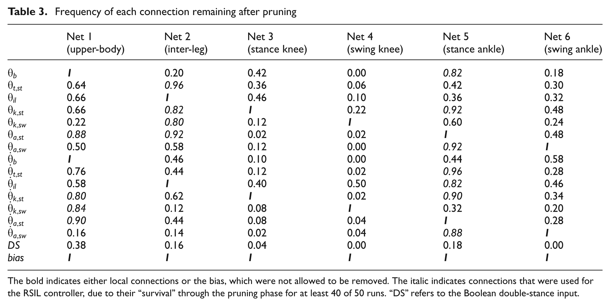
The bold indicates either local connections or the bias, which were not allowed to be removed. The italic indicates connections that were used for the RSIL controller, due to their “survival” through the pruning phase for at least 40 of 50 runs. “DS” refers to the Boolean double-stance input.

Several important observations may immediately be made. The upper-body, inter-leg and stance ankle controllers clearly require the most elaborate control, on average keeping 61%, 51% and 66% of non-local connections, respectively (calculated by averaging all non-bold values in each column). In comparison, the swing knee, stance knee, and swing ankle controllers kept only 8%, 18%, and 32% of non-local connections, respectively. This result is not surprising in light of the observed walking behaviors, as the swing knee trajectory is relatively consistent, the stance knee usually locked, and the swing foot behavior does not need elaborate control to prevent toe-scuffing nor to ensure proper heel-strike at the end of a step.

Another notable result is that all the network input variables (besides DS) proved to be useful for locomotion control, with their network connections frequently surviving the pruning process, but a given connection’s survival depended greatly on the network with which it was associated. For example, the connection from $θ_{k, sw}$ survived 22% of the time for Network 1 (upper-body) and 80% of the time for Network 2 (inter-leg), while the connection from ${\overset{\cdot}{θ}}_{k, sw}$ survived 84% of the time for Network 1 and 12% of the time for Network 2. Thus the position of the swing knee was found to be important for controlling the inter-leg angle, but not for controlling the upper body. In contrast, the velocity of the swing knee was found to be important for the control of the upper-body, but relatively unimportant for the control of the inter-leg angle.

As explained in Section 2.7.5, the connections of the RSIL controller consisted of those that were not pruned for at least 80% (40 of the 50) pruning phases. The result is that all input variables except $θ_{il}$ , ${\overset{\cdot}{θ}}_{b}$ , and DS were used as inputs for at least one of the six networks, but none of them for more than two, again reinforcing that the usefulness of an input variable depends on which joint it is being used to control.

Examination of Table 3 reveals that the control of the stance ankle (network 5) required the most non-local inputs, followed by the upper-body and inter-leg angles (networks 1 and 2). In contrast, the stance and swing knee and the swing ankle did not require any non-local inputs (networks 3, 4, and 6). Summarizing, networks 1, 2 and 5 of the RSIL controller ended up receiving 4, 4, and 7 non-local inputs, respectively, while the other three networks received zero, effectively acting as local PD controllers with fixed set points.

3.3 Controller benchmarks

We consider two fundamental ways to benchmark controller performance: stability and efficiency. Conveniently, the fitness function used in this study provides a measure of both. As mentioned earlier, at the end of each run, a tournament is held, and the winner is tested for 1000 fitness evaluations. We thus consider the percentage of fitness evaluations that result in a fall as the stability metric. For efficiency, it is straightforward to compute the dimensionless specific mechanical cost of transport $C_{mt}$ , defined as the amount of positive mechanical work required to move a unit weight a unit distance (Collins, Ruina, Tedrake, & Wisse, 2005; Srinivasan and Ruina, 2006). We average the $C_{mt}$ values computed over the 1000 runs as a final measure of efficiency.

Table 4 reveals several interesting results. The LPD controller, while not especially efficient, exhibits remarkable stability for such a minimalistic control scheme considering the ruggedness of the terrain, falling in as few as 7.3% of trials. With the full interconnectivity of the FIL controller comes a great improvement in efficiency—with $C_{mt}$ as low as 0.033 (0.044 average) and fall percentage as low as 2.0% (12.8% average). Considering that humans walking on level ground have a $C_{mt}$ of about 0.05 (Collins et al., 2005), this is a very good level of efficiency. It should be noted, however, that since the model is 2D, there is no need to expend energy to ensure lateral stability, as there is with humans. Although the SIL controllers only possessed an average of 39% as many non-local connections overall as the FIL controllers, the reduction in both efficiency and stability is relatively negligible. Indeed, the RSIL controllers, which incorporate only 19% of the non-local connections (15 out of 78), also performed impressively, with similar efficiency and stability.

Table 4.

Performance benchmarks of the various controller types

	$C_{mt}$ (mean/best)	Fall % (mean/best)
LPD	0.218±0.025/0.169	25.2±7.9/7.3
FIL	0.044±0.006/0.033	12.8±7.7/2.0
SIL	0.047±0.009/0.028	19.7±10.8/4.9
RSIL	0.043±0.003/0.038	10.4±4.6/3.6

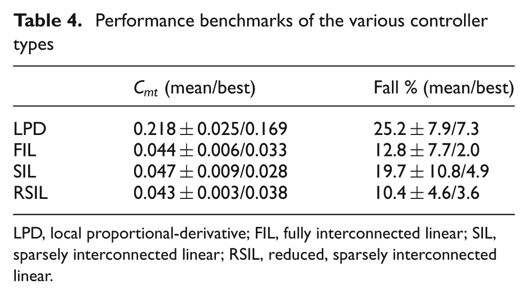
LPD, local proportional-derivative; FIL, fully interconnected linear; SIL, sparsely interconnected linear; RSIL, reduced, sparsely interconnected linear.

3.4 Walking behaviors

With the exception of the LPD framework, all EA runs evolved weight sets that exhibited qualitatively similar-looking walking behaviors. Example stick figures and kinematic plots are shown in Figures 5 and 6, respectively, as well as the Supplementary Video. The figures and video reveal a remarkably human-like gait pattern. Each stride, the upper-body undergoes a smooth rotation around 0°, with the amplitude adjusted to compensate for terrain unevenness. The stance thigh angle increases in a relatively linear manner, while the inter-leg angle increases relatively abruptly for the first half of the stride, and by a much smaller amount for the second half. The stance knee generally remains locked out, and the swing knee smoothly bends from 0° to between 60° and 90° and back to 0° during the first two-thirds of the stride, and remains locked out. The stance ankle angle increases linearly for the first two-thirds of the stride, and then abruptly starts to decrease, exhibiting a push-off behavior. The swing ankle behaves in a reasonable manner, experiencing a small disturbance as the swing knee locks out, and quickly decreases after the swing foot’s heel makes contact with the ground. The LPD-based walking motions appeared similar to those of the other frameworks, but the upper-body tended to lean forward, and the inter-leg angle increased more rapidly, which helps explain the reduced efficiency of LPD control.

Figure 5.

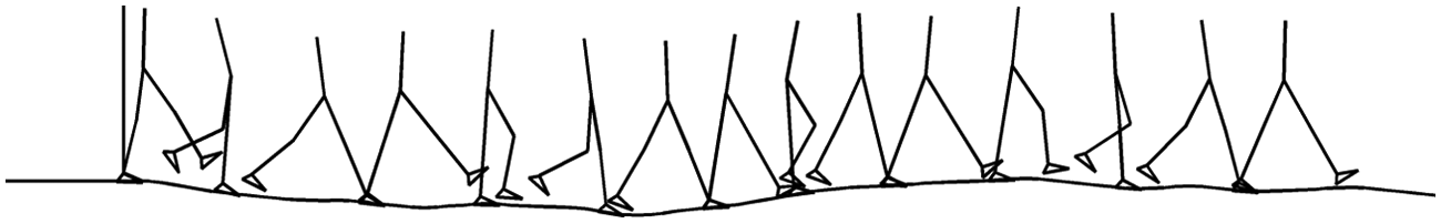
A sequence of walking steps for a particular fully interconnected linear (FIL) controller, starting with gait initiation. The time transpiring between each frame is 0.5 seconds.

Figure 6.

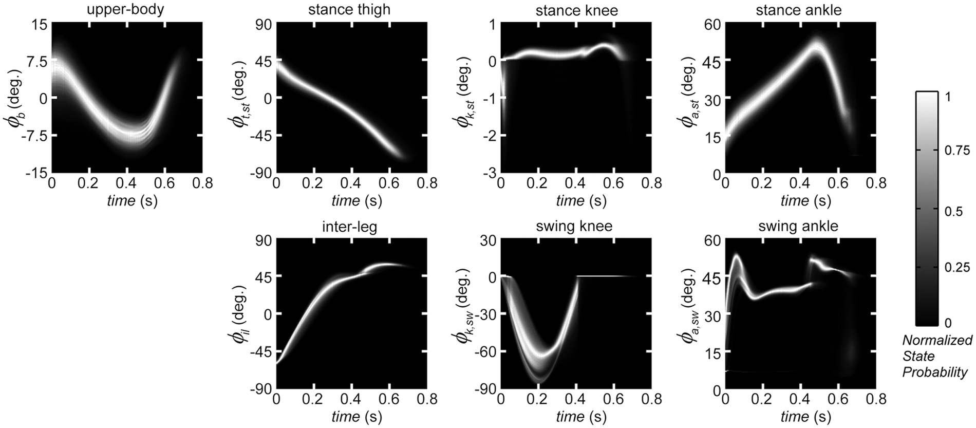
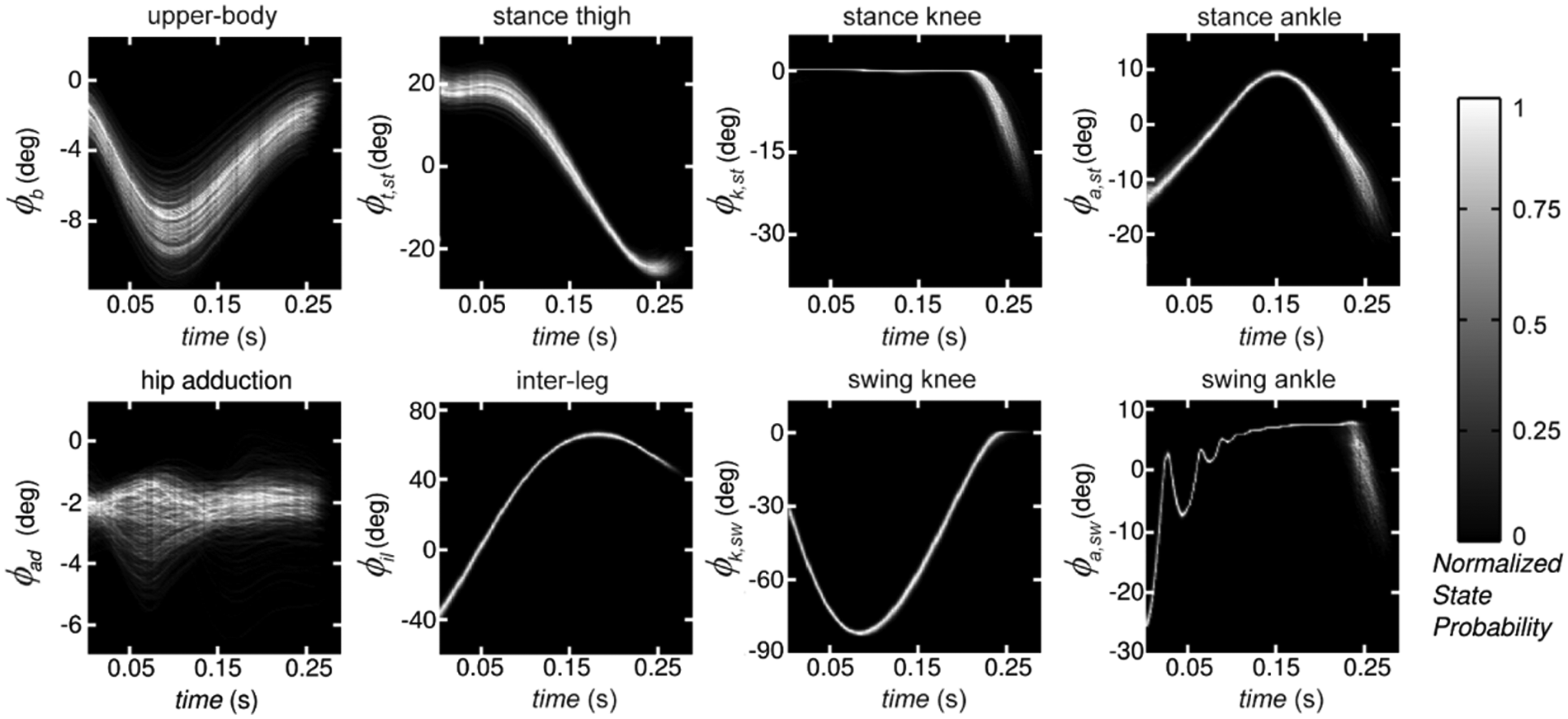
Averaged kinematics over thousands of strides for a typical fully interconnected linear (FIL) controller. The intensity of whiteness indicates how frequently the walker passed through a given state, with each time “slice” normalized relative to the most frequent state within the slice; 5000 successful walking trials (no falls) were used to generate the figure.

In addition to kinematic analysis, we also compared the controllers using intuitive metrics of the walking patterns, including mean speed, mean step length and mean percent double-stance (the percent of each stride during which both feet were on the ground). Specifically, for each of the tournament winners, we conducted 100 successful walking trials (no falls) and averaged the results, shown in Table 5. The standard deviations of the metrics were computed to give a measure of the variability of the behavior between tournament winners for each of the frameworks.

Table 5.

Metrics of walking behaviors

	Walking speed (m/s)	Step length (m)	Pct. double-stance (%)
LPD	1.50±0.14	0.762±0.045	8.29±1.46
FIL	1.44±0.08	0.966±0.031	5.59±1.22
SIL	1.42±0.08	0.941±0.051	5.38±1.47
RSIL	1.41±0.03	0.773±0.063	5.06±2.19

LPD, local proportional-derivative; FIL, fully interconnected linear; SIL, sparsely interconnected linear; RSIL, reduced, sparsely interconnected linear.

Table 5 reveals that both the average walking speeds and step lengths were generally consistent with a human walking at a slightly brisk pace, but the double-stance phase was notably briefer (∼20% is typical for humans) (DeLisa, 1998). The variability (standard deviations) of the various metrics was mostly small but not entirely insignificant, indicating that good walking performance can be achieved at a range of walking speeds and step lengths.

3.5 3D results

3.5.1 The 3D walker on slightly rough terrain

We next conducted experiments in which we generalized the 2D results to a 3D model, demonstrating the efficacy and scalability of the linear reactive controller. We follow the same procedure as the 2D experiments in order to demonstrate control of a 3D walker on slightly rough terrain (step-to-step terrain height standard deviations of about 0.36% leg-length). Slightly rough terrain provides a demonstration of walking on nearly flat ground, and helps prevent dangerous behaviors (sliding, tip-toeing, near-zero swing foot clearance) that can emerge when perfectly flat ground is used. See Appendix A for details on ground roughness. An LPD set of weights was chosen by hand to bootstrap the first generation of SIL controllers, as described in Section 2.7.4, and then the same EA was implemented to optimize the weights with minor differences as noted in Section 2.7.3.

Interestingly, the reduced set of connections based on the 2D SIL results worked extremely well in 3D also. The connections for the six shared actuators were taken directly from a 2D SIL run (identities only, not weight values), and a hip adduction actuator network was then added as described in Section 2.5.3. Stable 3D walking behaviors were readily evolved using this sparse network, with no additional design effort. Six runs were averaged together, and the evolution of fitness is shown in Figure 7.

Figure 7.

Results of the evolutionary algorithm (EA) optimization of a 3D walker, averaged over six runs. The upper three curves represent the maximum fitness±the standard deviation of maximum fitness values, and the bottom three curves represent the mean fitness±the standard deviation of mean fitness values.

Figure 7 shows that, with 1000 N·m·s of torque cost, the best 3D walkers in each generation were able to travel slightly over 50 m. An average walker could cover about 20 m, most of them falling before expending the available torque cost. Evaluation of tournament winners yielded a mean C_mt of 0.376±0.008. By comparison, ZMP-controlled bipeds such as ASIMO have a C_mt around 1.6 (Collins et al., 2005). Thus our 3D walkers are approximately four times more efficient, even though they are trained to walk over rough terrain. The tournament winner fell in 11.7% of trials.

Note that, compared with Figure 4, the evolution proceeds very quickly. Using the reduced set of weights helps to reduce the solution search space, meaning that only a few hundred generations are required for the fitness to approach its final value. This is a favorable result, as it quickly generates very stable walking controllers with minimal design effort for 3D bipedal locomotion, an extremely difficult control task. The similarity in both the procedure and the control framework between 2D and 3D models demonstrates the straightforward scalability of this method.

3.5.2 The 3D walker on rough terrain

Starting with the 3D controllers evolved for slightly rough terrain, the roughness of the terrain was gradually increased ten-fold over 800 generations, from step-to-step terrain height standard deviations of 0.36% leg-length to about 3.55% leg-length. Sample videos are included in Supplemental Online Materials.

Similar to Figure 6, kinematic data for one typical controller was generated by testing on 1000 different rough terrains. The averaged trajectories are plotted in Figure 8.

Figure 8.

Averaged kinematic data for a typical sparsely interconnected linear (SIL) 3D controller generated by testing on 1000 different rough terrains (no falls included).

There is less variability in these trajectories compared to those in Figure 6, possibly because of the higher walking speed (∼3 times faster than the 2D walker). The short step duration leaves little time to diverge from the trajectories shown, so the joints fall into very consistent limit cycles. The upper-body and hip adduction plots are noteworthy for having the most variable trajectories. The hip adduction plot has trajectories distributed over much of the plot area because this joint is used to control step width, which stabilizes lateral falls. This angle is therefore highly dependent on the terrain. The upper-body angle is the second-most diffuse, as it is also adjusted to compensate for unevenness.

The highest terrain roughness used during evolution was a step-to-step height standard deviation of about 3.55% leg length. The fall rate for the best individuals in the tournament on this level of roughness was very high (over 99% failed at some point before exhausting 1000 N·m·s of torque cost), so in order to more effectively evaluate the performance, a tournament was conducted on terrain with standard deviations of about 2.0% leg-length. The winner of this tournament had a mechanical cost of transport of C_mt=0.421±0.005, and a fall rate of about 16.7%.

4 Discussion

4.1 Linear reactive control for robotics

The linear reactive control approach presented in this study was shown to enable stable and efficient simulations of locomotion over rough terrain using both 2D and 3D models. From an algorithmic perspective, the control approach is “simple,” in that it relies only on a linear weighted sum of the sensory inputs, and requires no dynamic memory. From an optimization perspective, the control approach might be called “complex,” in that it requires dozens of weights to be tuned in order to establish a successful control network. Our view is that although the size of the search space is large, the algorithmic simplicity of linear reactive control is novel among bipedal walking controllers considering the level of stability and efficiency achieved.

It is not at all obvious that linear reactive control should be sufficient to enable biped walkers to negotiate rough terrain. Although hand-tuned controllers for the 3D “Cornell biped” and “Denise” have been shown to enable locomotion over flat terrain (Collins et al., 2005), and “Flame” can even handle small step-downs (Hobbelen and Wisse, 2009), walking over rough terrain requires considerably more adaptive behavior. In particular, results from previous studies have seemed to suggest that central pattern generators may be needed to entrain the oscillatory dynamics of the body/environment interaction (Taga, 1995a, 1995b). Importantly, the results of the present work demonstrate that 3D bipedal locomotion over rough terrain can be achieved with a control architecture consisting of little more than a weighted linear sum of sensor states. Although the present approach does not by itself afford any theoretical stability guarantees, the trajectories it generates are amenable to theoretic analysis in future studies.

The present work does not demonstrate that linear reactive control is the best controller for bipedal locomotion; it is indeed likely that a nonlinear controller could allow for at least marginally higher fitness behavior. The present work does, however, demonstrate that linear reactive control is a very good solution, especially given its very simple structure, which we consider to be a virtue (all things being equal, simple solutions are preferable). Furthermore, by maximizing the performance of linear control for bipedal locomotion, we can help to establish what benefits are being afforded by nonlinear control approaches.

The simulation results presented here make linear reactive control a favorable candidate for application to a robotic testbed. The problem, however, is that its reliance on numerical optimization to tune the network weights makes it challenging to implement in hardware: it is clearly infeasible to perform thousands of fitness trials in hardware, yet discrepancies between simulation and hardware will preclude direct transfer of simulation results. In a recent study, we investigated an approach to address this problem: various forms of noise and uncertainty, as well as a realistic actuation model, were introduced into the 3D model simulation (Locascio et al., in press). By randomly varying the biped’s dynamic parameters and terrain properties for each fitness evaluation, the weights must evolve such that the controller is robust to these deviations. Although additional measures are likely to be needed before effective hardware transfer can take place, we anticipate that this may be a useful approach to aid in crossing the “reality gap” (Jakobi, Husbands & Harvey, 1995; Zagal and Ruiz-del-Solar, 2007).

4.2 Extension from the 2D to the 3D model

A significant advantage of the approach used in this study is that it was relatively easy to scale up control of the 2D model to the 3D model. The 2D seven-link model was an invaluable tool for developing the control framework and efficient evolutionary parameters. However, this model bypasses some complex control issues—most importantly, lateral stability—that must be addressed for the case of 3D humanoid walking. It was therefore necessary to show that a linear reactive controller was truly a viable option for unsupported 3D walkers.

The expansion from 2D to 3D required the addition of one actuator control network for hip adduction, and the inclusion of up to ten more sensor inputs to each network, if a fully connected controller is desired. These changes were easy to implement as natural extensions of the 2D model, increasing the appeal of the linear reactive controller design. The most important non-trivial change required for the 3D controller was the interpretation of the “roll” and “yaw” values that were used as inputs to the hip adduction network. 3D walking, even on flat terrain, carries the risk of toppling laterally, in the direction transverse to the direction of travel. The 3D walker prevents lateral falling through hip adduction, i.e., widening or narrowing the step width. To address the symmetric nature of walking and enable this behavior, the signs of the roll and yaw angles and velocities had to be flipped whenever the left leg was the stance leg.

Aside from this lateral stability issue, the controller used in the 2D model was directly applicable to a 3D model with the addition of appropriate sensors and actuator networks. It is particularly noteworthy that the 2D SIL connections were directly applicable to the 3D model, perhaps implying a high degree of decoupling between forward and lateral control aspects of biped walking.

4.3 Bottom-up design using the fitness function

A significant advantage of the evolutionary optimization approach used in this study is the ease with which it allows characteristics of the controller to be adjusted, as well as its potential to be used for the design of controllers for different locomotion behaviors (e.g., running, jumping, turning, traversing steps, and gait initiation). However, it must be emphasized that the controller “design” is not carried out in the traditional top-down sense wherein the controller is synthesized through rigorous mathematical modeling and control systems engineering. Instead, the fitness function must be carefully formulated in such a way that the desired (high fitness) behavior emerges in a bottom-up sense as the EA optimizes the network weights.

In the current study, the fitness function was designed to not only ensure that the controller is stable and efficient, but also to reward improvement in an incremental way, thereby discouraging the optimization from falling into local minima. In the early stages of each EA run, all the selection pressure was on stability because the walker would fall before exhausting its joint torque cost $C_{τ}$ , much like a toddler focuses on standing upright and taking small steps forward before walking efficiently. Once individuals in the population were able to walk far enough to completely use the torque cost, efficiency became an important factor in the optimization. Increasing the value of $C_{τ}$ increases the relative importance of stability compared to efficiency, and vice-versa. Optimization also takes longer when $C_{τ}$ is increased because the biped may walk farther on any given fitness evaluation.

Another interesting aspect of the fitness function was its use of joint torque cost instead of mechanical energy expenditure. If mechanical energy expenditure were used, Equation 4 would simply be modified by multiplying the $| τ_{n} |$ term by ${\overset{\cdot}{ϕ}}_{jo int} (n)$ , where ${\bar{ϕ}}_{joint} = [ϕ_{h, st}, ϕ_{h, sw}, ϕ_{k, st}, ϕ_{k, sw}, ϕ_{a, st}, ϕ_{a, sw}]$ for the 2D model. We experimented with using mechanical energy expenditure, but found that led to gait patterns with overly stiff joints, e.g., locking out the swing knee and keeping the stance ankle relatively stiff, which is not surprising given that keeping ${\overset{\cdot}{ϕ}}_{joint} (n)$ small conserves energy. Moreover, joint torque cost may be a better reflection of true metabolic expenditure in humans, as well as a better reflection of battery power expenditure in robots. For example, consider a control strategy that involves fully extending the stance leg and “locking” the knee with a strong torque on the stance knee motor. Although it is clear that applying a strong torque implies metabolic exertion (in humans) or use of battery power (in robots), it accounts for no mechanical energy expenditure in this scenario, since the knee joint angle velocity would be zero. The joint torque cost metric addresses this issue by integrating only the absolute torque magnitude over time.

Finally, the particular controllers evolved in the present work are likely to owe part of their success to the fact that both 2D and 3D simulations were based on physical systems (a human and robot, respectively) specifically designed to exploit principles of passive dynamic walking (Hobbelen et al., 2008). For these systems, much of the locomotor computation is inherent in the physical interaction between the robot and the environment, leading to a large basin of attraction and hence aiding in optimization from start to finish. If a linear reactive approach were used to control other types of bipeds—ones that had been designed in the absence of passive dynamic principles—it is likely that the optimization would be more difficult and lead to less anthropomorphic walking patterns.

5 Conclusion

The linear reactive control approach presented in this study enables locomotion over rough terrain with remarkable stability, efficiency and human-like movement, especially considering the overall simplicity of the architecture. By using an EA to tune the weights, properties of the resulting gaits can be altered in a straightforward manner. Future studies may focus on implementing the approach in hardware, and also explore how different fitness functions can be used to enable the evolution of diverse behaviors such as speed control, jogging, running, turning and traversing stairs.

Footnotes

Appendix A: 3D terrain profile generation

In order to generate terrains for the 3D model, the random walk procedure had to be altered to produce surfaces. This was done using a constrained 2D random walk to build an m-by-n matrix of height values.

Starting on column 1 and proceeding to column n, the first row of nodes is produced using a standard 1D random walk with unity step size. Row 2 starts at column n and proceeds toward column 1. The entry at (2,n) is also a random-walk step from the entry at (1,n). The entry at (2,n−1) is based on the values at (1,n−1) and (2,n). If the two values are the same, we take another random-walk step. If they differ by more than 1, then an additional step away from those values is prevented. This keeps two values in the same column from diverging wildly. At the end of row 2 (back at column 1), we again proceed in row 3 from column 1 to column n, and continue the procedure.

Another matrix, this one of transposed dimensions n-by-m, is then produced in the same way. It is transposed and added to the first layer, and then each element in the resulting matrix is divided by two. This composition of layers cancels out any bias that may arise in the directions in which the layers were produced.

The surface is then smoothed by averaging using 2D windows with a side length of f nodes. This is effectively a low-pass filter determining the frequencies present in the surface. A higher f value results in more averaging, removing more high frequencies. In this study, we used f=5, and node spacings equal to those of the 2D terrain (0.1 m). Finally, the value of each point is multiplied by the scale factor, r, to determine the amplitudes. A perfectly flat terrain can be generated using r=0.0, but this could allow unsafe behaviors to evolve, such as near-zero swing foot heights. Instead, our “slightly rough terrain” uses r=0.002, which corresponds to step-to-step height standard deviations of about 0.36% leg-length. The highest roughness used during evolution used r=0.02, which results in a standard deviation of about 3.55% leg-length. The tournament in Section 3.5.2 used r=0.01, which results in a standard deviation of about 2.0% leg-length.

Additionally, it should be noted that the first 2 m of these terrains were perfectly flat to avoid a bootstrapping problem in which a difficult starting point on the terrain immediately caused falls. The terrain for the 2D model started perfectly flat up to the tip of the toes, but was rough immediately thereafter.

Appendix B: mathematical implementation of control architecture

Expressed mathematically, the output (motor torque) $τ_{n}$ of network n is computed as:

(5)

τ_{n} = \sum_{i = 1}^{m (n)} W_{net} (n, i) \cdot x (i)

$W_{net} (n, i)$ is the ith weight of network n, $x (i)$ is the signal coming from input node i, and $m (n)$ is the number of inputs for network n. There is one small but critical modification to Equation 5 for network 1, making it

(6)

τ_{1} = \sum_{i = 1}^{m (1)} W_{net} (1, i) \cdot x (i) - τ_{2}

This causes control of the upper-body to be effectively isolated from the activity of the swing hip’s actuator, enabling stable locomotion using the LPD control framework, which would not be possible using LPD control directly on $ϕ_{h, sw}$ and $ϕ_{h, st}$ . As is common with neural networks, all of the raw sensor states s are shifted and scaled to the range [−1, 1] with an affine transform:

(7)

x (i) = σ_{scale} (i) \cdot s (i) + σ_{shift} (i)

where $σ_{scale} (i)$ and $σ_{shift} (i)$ are the scaling and shifting parameters for sensor state i, respectively. For each of the 50 runs, these parameters were determined based on the minimum and maximum state values measured during a single fitness evaluation (in which a fall did not occur).

Acknowledgements

We thank Martijn Wisse for providing a copy of the Flame robot, associated CAD drawings, and other assistance.

Funding

This work was supported by the Director’s Research and Development Fund program of the Jet Propulsion Laboratory (California Institute of Technology), NSF awards IOS-0818414 and IOS-0846088 to MJZH, and the Graduate Student Research Program of the Jet Propulsion Laboratory (award number 10401 to MAL).

About the Authors

Joseph H Solomon is currently an adjunct assistant professor in the department of biomedical engineering at Northwestern University, Evanston, IL. He received a B.S. degree in aeronautical and astronautical engineering from the University of Illinois at Urbana-Champaign in 2001, an M.S. degree in mechanical engineering from the University of Illinois at Chicago in 2003, and a Ph.D. degree in mechanical engineering from Northwestern University in 2008. His research interests include evolutionary algorithms, neural networks, artificial general intelligence, biomimetic sensing, and bipedal locomotion.

Mark A Locascio received a B.S. degree in engineering from Harvey Mudd College (Claremont, CA) in 2005. He completed an M.S. degree in mechanical engineering from Northwestern University (Evanston, IL) in 2009, and received his Ph.D. degree in mechanical engineering from Northwestern University in 2012. He was a NASA GSRP fellow from 2010 to 2012. His research interests include evolutionary robotics, machine learning, control, and numerical methods.

Mitra J Z Hartmann is an associate professor at Northwestern University with a 50/50 joint appointment between the departments of biomedical engineering and mechanical engineering. She received a B.S. degree in applied and engineering physics from Cornell University, and a Ph.D. degree in integrative neuroscience from the California Institute of Technology. From 2000–2003, she was a postdoctoral scholar at the Jet Propulsion Laboratory in Pasadena, California, where she worked in the bio-inspired technology and systems group. Dr. Hartmann’s research interests involve understanding the mechanics and neuroscience of active sensing behaviors.

References

Bishop

C. M.

(1996). Neural networks for pattern recognition. Oxford University Press USA.

Braitenberg

(1984). Vehicles: Experiments in synthetic psychology. Cambridge, MA, MIT Press.

Byl

Tedrake

(2009). Metastable walking machines. International Journal of Robotics Research 28(8), 1040–1064.

Chevallereau

Abba

Aoustin

Plestan

Westervelt

E. R.

Canduas-de-Wit

Grizzle

J. W.

(2003). RABBIT: A testbed for advanced control theory. IEEE Control Systems Magazine 23(5), 57–79.

Chiel

H. J.

Beer

R. D.

(1997). The brain has a body: adaptive behavior emerges from interactions of nervous system, body and environment. Trends in Neurosciences 20(12), 553–557.

Chiel

H. J.

Ting

L. H.

Ekeberg

Hartmann

M.J.Z.

(2009). The brain in its body: Motor control and sensing in a biomechanical context. Journal of Neuroscience 29(41), 12807–12814.

Collins

S. H.

Ruina

(2005). A bipedal walking robot with efficient and human-like gait. Proceedings of the 2005 International Conference on Robotics and Automation, Barcelona.

Collins

S. H.

Ruina

Tedrake

Wisse

(2005). Efficient bipedal robots based on passive-dynamic walkers. Science 307, 1082–1085.

DeLisa

J. A.

(1998). Gait analysis in the science of rehabilitation. Darby, PA: Diane Publishing Co.

10.

Eiben

Smith

(2003). Introduction to evolutionary computing. Heilderberg: Springer.

11.

Garcia

Chatterjee

Ruina

Coleman

(1998). The simplest walking model: Stability, complexity, and scaling. Journal of Biomechanical Engineering 120(2), 281–288.

12.

Geyer

Herr

H. M.

(2010). A muscle-reflex model that encodes principles of legged mechanics produces human walking dynamics and muscle activities. IEEE Transactions on Neural Systems and Rehabilitation Engineering 18(3), 263–273.

13.

Haavisto

Hyötyniemi

(2004). Simulation tool of a biped walking robot model. Helsinki University of Technology, Control Engineering Laboratory.

14.

Hasegawa

Arakawa

Fukuda

(2000). Trajectory generation for biped locomotion robot. Mechatronics 10(1–2), 67–89.

15.

Hobbelen

D. G. E.

Wisse

(2008a). Ankle actuation for limit cycle walkers. The International Journal of Robotics Research 27(6), 709–735.

16.

Hobbelen

D. G. E.

Wisse

(2008b). Controlling the walking speed in limit cycle walking. The International Journal of Robotics Research 27(9), 989–1005.

17.

Hobbelen

D. G. E.

Wisse

(2008b). Swing leg retraction for limit cycle walkers improves disturbance rejection. IEEE Transactions on Robotics 24(2), 377–389.

18.

Hobbelen

D. G. E.

Wisse

(2009). Active lateral foot placement for 3D stabilization of a limit cycle walker prototype. International Journal of Humanoid Robotics 6(1), 93–116.

19.

Hobbelen

D. G. E.

de Boer

Wisse

(2008). System overview of bipedal robots Flame and TUlip: Tailor-made for limit cycle walking. IEEE/RSJ International Conference on Intelligent Robots and Systems. Nice, pp. 2486–2491.

20.

Jakobi

Husbands

Harvey

(1995). Noise and the reality gap: The use of simulation in evolutionary robotics. In Moran

Moreno

Merelo

J. J.

Chacon

(Eds.), Advances in artificial life, volume 929, pp. 704–720. Berlin: Springer-Verlag.

21.

Kuo

A. D.

(2002). Energetics of actively powered locomotion using the simplest walking model. Journal of Biomechanical Engineering 124, 113–120.

22.

Locascio

M. A.

Solomon

J. H.

Hartmann

M.J.Z.

(in press). Linear reactive control of bipedal walking in the presence of noise and uncertainty. Adaptive Behavior. Published online before print August 31, 2012, doi: 10.1177/1059712312453059.

23.

Manoonpong

Geng

Kulvicius

Porr

Wörgötter

(2007). Adaptive, fast walking in a biped robot under neuronal control and learning. PLoS Computational Biology 3(7), 1–15.

24.

McGeer

(1990). Passive dynamic walking. The International Journal of Robotics Research 9(2), 62–82.

25.

Mondada

Floreano

(1995). Evolution of neural control structures: Some experiments on mobile robots. Robotics and Autonomous Systems 16, 183–195.

26.

Nolfi

Floreano

(2004). Evolutionary robotics: The biology, intelligence, and technology of self-organizing machines. Cambridge, MA: The MIT Press.

27.

Ono

Takahashi

Shimada

(2001). Self-excited walking of a biped mechanism. The International Journal of Robotics Research 20(12), 953–966.

28.

Paul

(2005). Sensorimotor control of biped locomotion. Adaptive Behavior 13(1), 67–80.

29.

Reil

Husbands

(2002). Evolution of central pattern generators for bipedal walking in a real-time physics environment. IEEE Transactions on Evolutionary Computation 6(2), 159–168.

30.

Sims

(1994). Evolving virtual creatures. Proceedings of the 21st annual conference on Computer graphics and interactive techniques, New York.

31.

Smith

(2009). Open Dynamics Engine. Retrieved January 8, 2010, from www.ode.org.

32.

Solomon

J. H.

Wisse

Hartmann

M.J.Z.

(2010). Fully interconnected, linear control for limit cycle walking. Adaptive Behavior 18(7), 492–506.

33.

Srinivasan

Ruina

(2006). Computer optimization of a minimal biped model discovers walking and running. Nature 439(5), 72–75.

34.

Srinivasan

Westervelt

E. R.

Hansen

A. H.

(2009). A low-dimensional sagittal-plane forward-dynamic model for asymmetric gait and Its application to study the gait of transtibial prosthesis users. Journal of Biomechanical Engineering 131(3), 031003.

35.

Strogatz

S. H.

(2000). Nonlinear dynamics and chaos. Cambridge, MA: Westview Press.

36.

Taga

(1995a). A model of the neuro-musculo-skeletal system for human locomotion. I. Emergence of basic gait. Biological Cybernetics 73(2), 97–111.

37.

Taga

(1995b). A model of the neuro-musculo-skeletal system for human locomotion. II. Real-time adaptability under various constraints. Biological Cybernetics 73(2), 113–121.

38.

Taga

Miyake

Yamaguchi

Shimizu

(1993). Generation and coordination of bipedal locomotion through global entrainment. Proceedings of the International Symposium on Autonomous Decentralized Systems, Kawasaki.

39.

Taga

Yamaguchi

Shimizu

(1991). Self-organized control of bipedal locomotion by neural oscillators in unpredictable environment. Biological Cybernetics 65, 147–159.

40.

Terdiman

(2003). OPCODE. 1.3. from http://www.codercorner.com/Opcode.htm.

41.

Vaughan

E. D.

Di Paolo

E. A.

Harvey

(2004). The evolution of control and adaptation in a 3D powered passive dynamic walker. Proceedings of the Ninth International Conference on the Simulation and Synthesis of Living Systems, Boston, MA.

42.

Vukobratović

Borovac

(2004). Zero-moment point—Thirty years of its life. International Journal of Humanoid Robotics 1(1), 157–173.

43.

Winter

D. A.

(1991). Biomechanics and motor control of human gait: Normal, elderly and pathological. Waterloo, ON: University of Waterloo Press.

44.

Wisse

(2008). Deliverable 1.2, Hardware Specifications of EU FP6 Project ESBiRRo, TU Delft.

45.

Wisse

Schwab

A. L.

(2005). First steps in passive dynamic walking. Proceedings of the International Conference on Climbing and Walking Robots, London.

46.

Zagal

J. C.

Ruiz-del-Solar

(2007). Combining simulation and reality in evolutionary robotics. Journal of Intelligent & Robotic Systems 50(1), 19–39.

Supplementary Material

Please find the following supplemental material available below.

For Open Access articles published under a Creative Commons License, all supplemental material carries the same license as the article it is associated with.

For non-Open Access articles published, all supplemental material carries a non-exclusive license, and permission requests for re-use of supplemental material or any part of supplemental material shall be sent directly to the copyright owner as specified in the copyright notice associated with the article.

0.00 MB

39.35 MB