Evolution of reflexive signals using a realistic vocal tract model

Abstract

We introduce a model of the evolution of reflexive primate signals that incorporates a realistic vocal tract model for generating the signals. Signaler neural networks receive signal types as inputs and produce vocal tract muscle activations as outputs. These muscle activations are input to a model of the primate vocal tract, generating real sounds. Receiver neural networks receive spectrograms of these sounds as inputs and produce signal type classifications as outputs. Incorporating a realistic vocal tract has a substantial effect on the types of signals that can evolve. Compared to a model with abstract signals, the realistic model signals are more similar and have more correlated elements. The realistic, embodied model also exhibits more variability in rate of adaptation, usually adapting more slowly. This may be explained by the more jagged fitness landscapes in the realistic model. The realistic signals also tend to be quiet. Environmental noise results in louder signals but makes the evolutionary process even slower and less robust. These results indicate that signal evolution with a more realistic genotype–phenotype mapping can differ substantially from evolution with abstract signals. Including realistic signal generation mechanisms may enable computational models to provide greater insights into natural signal evolution.

Keywords

Embodiment evolution motor control neural network vocal signals computational model

1 Introduction

1.1 Reflexive vocal signals in primates

Non-human primates produce a variety of vocal signals that indicate an animal’s current state with regard to emotion, arousal, social interaction, and so on. Some of the functions served by these vocal calls include alarm, protest, aggression, play, social contact, separation, social bonding, and food preference (Arnold, Pohlner, & Zuberbühler, 2008; Benz, 1993; Biben, Symmes, & Masataka, 1986; Elowson, Tannenbaum, & Snowdon, 1991; Ploog, 1992; Seyfarth, Cheney, & Marler, 1980a,b; Talmage-Riggs, Winter, Ploog, & Mayer, 1972; Winter, Ploog, & Latta, 1966). The ability to appropriately use these vocalizations is clearly related to an animal’s fitness. For example, experimental deafening of squirrel monkeys can lead to at least a temporary increase in violent encounters with other monkeys and can lead to a downgrade in the deafened monkey’s status in the dominance hierarchy (Talmage-Riggs, Winter, Ploog, & Mayer, 1972).

Similarities across different primate species’ vocal systems have been observed (Masataka, 1983a; Snowdon & Pola, 1978) and the acoustic distinctiveness of call types has been argued to be demonstrated by the high reliability across human listeners in coding the vocalizations (Talmage-Riggs et al., 1972). Primate vocalizations, apart from human speech, are predominantly phonation-based, that is, based on production of sound at the larynx (Lieberman, 1968; Owren & Goldstein, 2008; Owren & Rendall, 2001), though there are some exceptions such as lip smacking (Ghazanfar, Takahashi, Mathur, & Fitch, 2012). For example, Goeldi’s monkeys produce two types of alarm calls, with the frequency range being the primary acoustic feature distinguishing the two types (Masataka, 1983a). Similarly, fundamental frequency within a signal appears to be a main distinguishing factor for how Japanese macaques respond to alarm calls (Masataka, 1983b). Adult pygmy marmosets produce two types of trills, used for different purposes, having similar fundamental frequency and apparently differing primarily in duration (Snowdon & Pola, 1978). Duration has also been found to be an acoustic feature that can distinguish vervet monkeys’ snake alarm calls from eagle alarm calls, with the repeating portions of the snake alarm calls being on average longer than those of the eagle calls (although differences in upper vocal tract filtering appear to also play a role in distinguishing these signals from each other) (Owren & Bernacki, 1988). Besides duration, vervet alarm calls tend to differ in pitch, temporal patterning of phonation, and whether they contain ingressive portions (Seyfarth, Cheney, & Marler, 1980a,b). Squirrel monkey calls also have been described as varying in a variety of predominantly phonatory features, including amplitude, duration, fundamental frequency, fundamental frequency contour, and temporal patterning of phonation (Winter, Ploog, & Latta, 1966). Finally, in further support of the laryngeal basis of many non-human primate calls, it has been found that a discriminant analysis based on fundamental-frequency-related features can be used for within-species discrimination of which food types have elicited tamarins’ vocalizations (Benz, 1993). Thus, it appears to be the case that across primate species, fundamental frequency, fundamental frequency contour, duration, amplitude, and other phonation-related acoustic variables form the primary basis for within-species differentiation of vocalizations that serve different functions.

The required laryngeal and respiratory motor patterning is controlled by neural circuitry in the brainstem (Jürgens, 2002). Auditory feedback appears to play only a minimal role; deafening of squirrel monkeys appears not to change the structure of their calls or which calls are produced under which eliciting situations. Deafening does affect call amplitude as well as the monkeys’ social interactions therefore affecting the frequency of different call types (Talmage-Riggs et al., 1972). The brainstem circuits responsible for the acoustic forms of the vocalizations appear to be largely innate, depending very little on learning, at least compared to human speech (Fischer & Hammerschmidt, 2010; Herzog & Hopf, 1984; Owren & Rendall, 2001; Winter, Handley, Ploog, & Schott, 1973). For example, it has been shown that infant vervet monkeys produce vocal calls, including screams and “whrrs”, that are acoustically similar to their adult counterparts (Seyfarth & Cheney, 1986), and human infants produce cries from birth. These features make it reasonable to call these vocal productions “vocal reflexes” (Talmage-Riggs et al., 1972). (Note that there are other calls, such as vervet grunts, that do show some significant acoustic changes over the course of infant development, though even the grunts produced at birth share a number of acoustic features with adult grunts; Seyfarth & Cheney, 1986.) The minimal role of the forebrain in patterning the vocalization and minimal reliance on learning sets the motor control for reflexive signals apart from that of human speech (Jürgens, 2002). Accordingly it is likely that the neural networks responsible for these reflexive calls are comparable to the reflex circuits and central pattern generators in the vertebrate spinal cord and brainstem, such as those involved in locomotion, breathing, and feeding (Barlow, Lund, Estep, & Kolta, 2009; Bass & Remage-Healey, 2008; Delvolvé, Branchereau, Dubuc, & Cabelguen, 1999; Grillner, 1982; Grillner & Wallen, 1985; Ijspeert, 2008; MacKay-Lyons, 2002; Miller, 1972; Pearson, 1995; Wheatley, Jovanović, Stein, & Lawson, 1994). As such, variations in these vocal productions are likely due to evolutionary processes rather than individual or social learning. On the perception side, responses to these signals appear to be at least partly innate. Squirrel monkeys reared in social isolation show appropriate responses to alarm calls typically made in response to bird predators as opposed to land predators and as opposed to a control, non-alarm sound (Herzog & Hopf, 1984). This being said, on the perception side learning does appear to play a more key role than it does in production (Masataka, 1983b).

Reflexive vocal signals are of particular interest because they represent the only, or at least the primary, means of vocal communication in non-human primates and appear to be preserved to some extent in humans, in the form of cries, shrieks, and laughter (Bryant & Aktipis, 2014; Jürgens, 1992; Lieberman, Harris, Wolff, & Russell, 1971; Oller, 2000; Oller et al., 2013), which are also innate, brainstem-based, and universal within the species. Furthermore, there is evidence suggesting that human speech, which relies heavily on neocortical involvement, may build upon the limbic system and brainstem circuitry responsible for producing reflexive signals, and it has been proposed that these non-human primate vocal signals are precursors to prosody in human speech (Jürgens, 2002; Ploog, 1992; Schulz, Varga, Jeffires, Ludlow, & Braun, 2005).

1.2 Previous models of the evolution of realistic acoustic signals

A number of computational models have addressed the evolution of signaling and receiving agents (Wagner, Reggia, Uriagereka, & Wilkinson, 2003), showing how signaling systems can evolve under a variety of conditions. Much of this work has modeled the signalers and receivers as neural networks with connection weights being genetically encoded. Most of the time the models are designed so that signals are arbitrary vectors (e.g. Cangelosi & Parisi, 1998; Krakauer & Johnstone, 1995; Levin, 1995; MacLennan & Burghardt, 1994; Nowak & Krakauer, 1999; Smith, 2002; Wagner et al., 2003; Werner & Dyer, 1992) rather than realistic signals such as gestures or vocalizations. Similarly, receiving agents are rarely required to process realistic signals.

There are a handful of exceptions that do make progress toward using more realistic signals. One example is a model by Di Paolo (2000) that used a genetic algorithm to evolve an acoustic communication system between two agents who moved about in a two-dimensional space and whose fitness depended on the ability to maintain proximity to each other. Each agent’s genome encoded parameters such as individual connection weights, neuronal biases, and decay rates in a neural network that generated and perceived simple acoustic signals. The signals took the form of a single frequency that varied continuously in amplitude over time. Across space, the signal amplitude dropped off with the squared distance from the sound source. The sound amplitude also attenuated when it passed through an agent’s body. These two physical properties created a shadowing effect. The use of acoustic signals had consequences for the types of strategies that the agents evolved, such as turn-taking patterns, which presumably were adaptive because they reduced interference between the two agents’ signals, and signals that tended to correlate with the agents’ angular movements, which was possible because of the shadowing properties of sound in the embodied simulation. By taking into account the physical properties of sound, in particular its change in amplitude as a function of distance and interference from a physical body, the work demonstrated how the physical embodiment of a signal can strongly affect the features of a communication system. This evidence that qualitatively different results can be obtained when the physical embodiment of a signal is incorporated into a model helps motivate the approach taken here, which focuses on how physical generation of acoustic signals by a primate vocal tract can affect the evolution of a communication system. In a neural network model by Bocchi, Lapi, and Ballerini (2010), signalers’ upper vocal tract (i.e. the portions of the vocal tract located above the larynx) configurations for each of five vowel signals were genetically encoded. Each signaler was paired with a receiver who learned, via a supervised neural network, to identify the signaler’s vowels. In other words, signal production was purely genetically encoded and signal perception was learned from scratch at each generation. The model successfully evolved accurate communication, even in the face of noise at the production or at the signal level. The work thus demonstrates the feasibility of evolving a control system for a realistic vocal tract model. However, its focus is on speech signals, specifically vowel sounds, and given this goal, its genetic encoding of signal production is unrealistic since the mapping from linguistic meaning to vocal tract configurations in human speech appears to be learned, rather than genetically fixed (De Saussure, 1983; Hockett, 1960; Oller, 2000; see Chater, Reali, & Christiansen, 2009, for a related computational argument regarding the evolution of language generally). Our goal here is to model the evolution of reflexive signals, a biologically simpler and evolutionarily broader class of vocal signals that includes most if not all non-human primate vocalizations as well as human screams, cries, and laughs. Given this goal, the focus should be on phonation-based patterns, modeling patterns of sound production at the larynx rather than patterns of filtering of a periodic sound source by the upper vocal tract (the latter is appropriate for modeling differences among vowel types in a speech system but not for differentiating among reflexive human and non-human primate vocalizations).

Incorporation of a realistic vocal tract model for sound production is much more common in work focused on speech sound learning and the cultural evolution of speech sound systems (De Boer, 2000, 2001; Heintz, Beckman, Fosler-Lussier, & Ménard, 2009; Howard & Messum, 2011; Kanda, Ogata, Komatani, & Okuno, 2008; Kröger, Kannampuzha, & Kaufmann, 2014; Kröger, Kannampuzha, & Neuschaefer-Rube, 2009; Miura, Yoshikawa, & Asada, 2012; Moulin-Frier, Nguyen, & Oudeyer, 2014; Nam, Goldstein, Giulivi, Levitt, & Whalen, 2013; Oudeyer, 2005, 2006; Warlaumont, 2013; Warlaumont, Westermann, Buder, & Oller, 2013; Westermann & Miranda, 2004; Yoshikawa, Asada, Hosoda, & Koga, 2003). One question of interest has been whether the “articulatory/energetic cost for vocalizations” (Oudeyer, 2005) and the perceptual distinctiveness of various sounds to the human auditory system will affect vocal learning and the cultural evolution of speech sound systems. For example, a study by Oudeyer (2005) focused on the emergence of a syllable inventory among a group of agents via inter-generational learning. More-difficult-to-generate sounds were harder for the agents to remember. Difficulty was a function of how much the vocal tract articulators had to move away from a fixed frame of neutral jaw oscillation (MacNeilage, 1998). Oudeyer’s model also took into account the particular features of how sound is processed by the human auditory system, so that there was pressure to converge on perceptually distinguishable sounds. In other words, both perceptual and motor features of the human body affected the speech sound systems upon which the agents ultimately converged. After a period of cultural evolution, the model had syllable inventories with properties similar to those observed in human languages. Relatedly, work by Nam, Goldstein, Giulivi, Levitt, and Whalen (2013) demonstrated, using a realistic upper vocal tract model, that the relative frequencies of various consonant–vowel combinations in infant babbling and adult speech may be due primarily to the physiological requirements of the consonant and vowel gestures: consonants and vowels that involve similar vocal tract configurations are more likely to co-occur. These studies thus support the idea that the physiology of the vocal tract, and the particularities of the articulatory-acoustic mapping, matter to the emergence of vocal signals. However, they focus on cultural speech sound evolution, which is likely to have relied much more on learning processes than the evolution of reflexive signals (at least as far as production is concerned) and also involves upper vocal tract (e.g. lip and tongue) movements to a greater extent than reflexive vocal signals, which rely primarily on control of thelarynx.

With regard to modeling reflexive signal perception, work by Ryan, Phelps, and Rand (2001) has incorporated a high degree of realism. They focused on the evolution of perception by female túngara frogs of male frogs’ mating signals. They evolved the connection weights of a simple recurrent neural network using a genetic algorithm where fitness depended on the ability to accurately detect which calls came from members of the same species and which belonged to other species. The inputs to the neural networks were spectrograms of realistic synthetic frog calls which were synthesized by manipulating seven acoustic parameters. These synthesized signals had previously been shown to elicit appropriate responses from real female frogs. The computational model accounted well for patterns observed in real frogs’ responses to synthesized vocalizations and supported the idea that the evolutionary history of being selected based on ability to perceive ancestors’ mating calls had effects on the way the species currently classifies signals. Thus, the use of realistic vocal signals in the model enabled more direct comparison with real animals’ behaviors and led to novel insights into real animals’ communication systems. Note, however, that the focus was exclusively on signal perception; evolution of the males’ call productions was not addressed. Our approach aims to extend this work by focusing not only on the perception of realistic vocal signals but also on their production.

1.3 Overview of the present study

It is important to move toward development of models of reflexive signal evolution that incorporate realistic signaling channels. The speed and form of evolution of signalers and perceivers is likely to be affected by constraints imposed both by the individuals’ physiology and by physical (e.g. acoustic) factors (Chiel & Beer, 1997). For example, physiological and physical constraints may make evolution of signaling more or less robust, or may affect the number of signals that can evolve. As was observed for Ryan et al.’s túngara frog model, we can expect that incorporating more realism will eventually lead to an improved ability to relate models of reflexive signals to real animal signals. We also expect that such work will eventually benefit the development of robots that communicate vocally (Parisi, 1997; Wagner et al., 2003). Creating a more realistic model of the evolution of neural control of reflexive vocalizations by the vocal tract will also pave the way for models of vocal learning to take into account the existing neural circuitry that is phylogenetically older than the circuitry used for speech-related vocal learning.

In this paper we present a study comparing the genetic evolution of communicative signals when the signals are made with a simulated primate vocal tract compared to when they are purely abstract vectors. The long-term goal is to move toward a computational model of how reflexive vocal signals might have evolved in the primate lineage. As far as we know this is the first computational model of reflexive vocal signal evolution to include a realistic mammalian vocal tract, focusing on phonatory components. It is also unique in that it explicitly compares how evolution progresses in simulations where signals are made realistic in this way versus where signals are abstract vectors.

Since the focus of this initial study is to introduce a realistic vocal sound generation apparatus into the modeling process, we simplify many other aspects of communication evolution. For example, we separate producers and receivers into distinct populations, and we assume that fitness is based on communication success, rather than letting the value of communication emerge from more natural interactions between agents and their environments, as these have already been the focus of a number of previous computational models (e.g. Di Paolo, 2000; Marocco & Nolfi, 2007; Quinn, Smith, Mayley, & Husbands, 2003; Werner & Dyer, 1992).

The simulation and analysis code are available at https://github.com/AnneSWarlaumont/NNVocEvo.

2 Methods

This study compares two types of models. In one of the models, signals are purely abstract vectors. We will call this the abstract model. In the other type of model, signals are created by simulation of the human vocal tract, so the sounds are more realistic with respect to how primate vocal signals are produced and perceived. We will call this the realistic model. The vocalization synthesis introduces a nonlinear transformation between signaler output and receiver input. These differences are highlighted in Figure 1.

Figure 1.

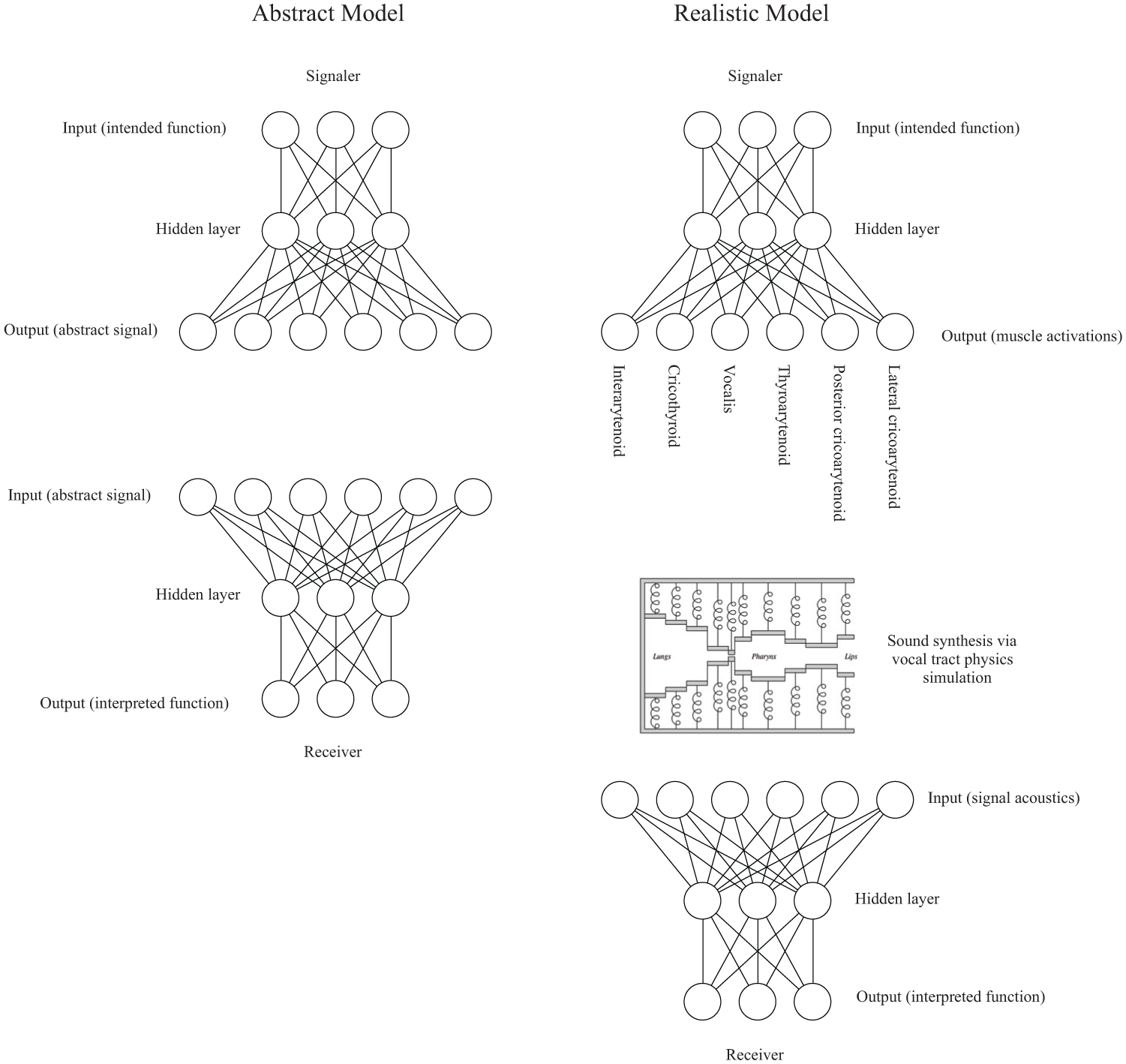
The left side shows how communication between a signaler and receiver takes place in the abstract model. One of the signaler’s intended function nodes is activated. That activity propagates through weighted connections to a hidden neuron layer and then to an output layer. The output layer activations constitute the abstract signal. These activations are directly given to the receiver as input node activations. The receiver’s input activity propagates through weighted connections to the hidden layer and then through weighted connections to the output layer. The most active of the receiver’s output nodes is the signal function as interpreted by the receiver. If this matches the signaler’s intended function, it is considered a successful signaling episode. The right side of the figure shows how communication between a signaler and receiver takes place in the realistic model. Instead of signaler outputs making up the signal itself, signaler outputs determine the activation levels for the six laryngeal muscles of the articulatory synthesizer. Vocal tract simulation is used to generate a synthesized vocalization. That synthesized vocalization is converted into a spectrographic representation, which is what is given as input to the receiver. The schematic illustration of the vocal tract model is copied with permission from Figure 2.1 of Boersma (1998). The original caption for that part of the figure is: “Simplified mid-sagittal view of our model of the speech apparatus (not drawn to scale). The model features a sequence of 89 straight tubes with walls consisting of masses and springs. The leftmost of these tubes is closed at the diaphragm, the rightmost tubes form the openings between the lips (and between the nostrils, which are not shown) and are open to the atmosphere, where fluctuations in the airflow are radiated as sound. The glottis is represented by two tubes (shown as one here), which are treated exactly the same way as all other tubes. The speech muscles can alter the rest positions and the tensions of the springs. Some of the masses are connected with springs to their nearest neighbors. Not shown are: the coupling springs that connect masses to their neighbors; the springs and masses in the z-direction (perpendicular to the paper); the nasal tract.”

Twenty repetitions of each model were run for 500 generations for a total of 40 simulations. The population size of each simulation was held constant at 100 signalers and 100 receivers. Each signaler is a three-layer feedforward neural network that takes one of three intended functions as input and produces a series of activations as output. In the abstract model, these output activations serve as the signal. In the realistic model, the output activations are interpreted as laryngeal muscle values that determine the behavior of the vocal tract simulator. The vocal tract simulation translates the muscle activations into acoustic output. Abstract model receivers take the signalers’ output activations directly as input. Realistic model receivers on the other hand take spectral information about the synthesized vocalization sounds as input. Receivers transform their input into guesses about which of the three possible functions was the signaler’s intended function. A genetic algorithm evolves the signaler and receiver neural network connection weights. Fitness is based on accuracy of matching between the producers’ inputs and the receivers’ most active outputs. Each of these components is described in more detail in the following subsections.

2.1 Generation of realistic and abstract signals

For the realistic model, we used the articulatory synthesizer described in detail in Boersma (1998) and available in Praat (Boersma & Weenink, 2010) (Figure 1). The synthesizer is intended to be a biologically realistic model of the human vocal tract and treats it as an air-filled tube bounded by walls of damped mass–spring systems. Muscle activation levels affect the parameters of the vocal tract walls, including resting positions, lengths, spring constants and damping constants. The pressure and airflow within the tube is calculated based on fluid dynamics conservation laws. The time-varying air pressure at the mouth is recorded as the sound output of the simulator and is saved as a .wav file. We chose this particular synthesizer because it includes a detailed representation of the larynx based on an established laryngeal model (Ishizaka & Flanagan, 1972), and it was readily and freely available (although there are a number of other articulatory synthesizers, many focus primarily on the upper vocal tract, i.e. the sections above the larynx, without realistically representing the laryngeal region). Note that while much of the laryngeal model is based on features of Ishizaka and Flanagan’s model, there are a number of additional complexities (see Section 2.7 of Boersma, 1998, for a detailed description).

Each vocal tract simulation and hence each realistic model signal lasted 0.5 s. The Lungs parameter, which controls the volume of air in the lungs, was set to 1 at time 0 s and decreased linearly to 0 at time 0.5 s. Depending on the state of the laryngeal muscles, which have nonlinear effects on vocal fold vibration, these lung settings will in some cases produce voiced sound and in other cases produce no sound at all or only a whisper-like breathiness. Laryngeal muscle activations were held constant throughout the 0.5 s time period. The following six laryngeal muscle activations were set to the levels specified by the signaler network’s output neuron activations: interarytenoid, cricothyroid, vocalis, thyroarytenoid, posterior cricoarytenoid, and lateral cricoarytenoid. These are all the laryngeal muscles included in the synthesizer. Activation of these muscles modifies the equilibrium positions and the tensions of the walls of the laryngeal portion of the vocal tract tube (Boersma, 1998). For simplicity in this initial study, non-laryngeal muscles, such as those affecting the tongue, lips, and jaw, were not activated. Our focus on laryngeal muscles was motivated by the fact that the reflexive primate vocal signals that are the focus of this study are primarily phonation-based, meaning that the signals’ characteristic acoustics are rooted in the way sound is produced at the larynx (Lieberman, 1968; Owren & Goldstein, 2008).

After running the vocalization synthesizer, the resulting sound waveform was transformed into a mel-scale power spectrogram with two time bins and three frequency bins ranging from 20 to 2000 Hz and centered at 433, 846.1, and 1306.3 Hz, using Ellis’s toolbox for MATLAB (Ellis, 2007). Although humans can hear up to about 20,000 Hz, since we wanted to use only a small number of elements to describe the spectrogram, we opted to focus on the lower frequency portions of the signal, which carry the most power in human vocalization. The spectrogram was then normalized by dividing each pixel’s power by 5 × 10¹¹, which, based on pilot explorations, scaled the values down to a range that was roughly between 0 and 1.

For simulations that used abstract, non-embodied signals, the signaler network’s six outputs were made to range from 0 to 1 by adding 1 to each value then dividing by 2. The resulting set of values served as the signal itself.

2.2 Signaler neural network

Each individual signaler was a three-layer feedforward neural network. There were three input nodes, equal to the number of signal functions. Signal functions can also be thought of as meanings, though we avoid the use of the term “meaning” in this paper as we do not wish to imply that reflexive primate vocal signals are referential (Oller & Griebel, 2014). Signal functions were represented in a localist manner with [1 0 0], [0 1 0], and [0 0 1] representing the first, second, and third signal functions respectively.

The input nodes were connected to a three-node hidden layer, which was in turn connected to a six-node output layer. Input node activations were multiplied by their connection weights to the hidden layer nodes, summed, and input to a hyperbolic tangent transfer function to obtain the hidden node activations. Hidden node activations were then multiplied by their weights to the output layer. Output nodes had a linear transfer function with a slope of 1 and an intercept of 0 that saturated at values of −1 and 1 (i.e. each output node’s weighted inputs were added together and the output was set to be the value of this sum except that if the sum was less than −1 the output was set to −1 and if the sum was greater than 1 the output was set to 1).

Neural network connection weights were determined by the individual’s genes (see Section 2.5 below) and did not change over the lifespan of an individual.

2.3 Receiver neural network

Each receiver also consisted of a three-layer feedforward neural network. There were six input nodes, equal to the number of elements in a signal. These input nodes were connected to three hidden nodes, which were connected to three output nodes, one for each signal function. Hidden layer nodes had a hyperbolic tangent transfer function. Output nodes had a linear transfer function with a slope of 1 and an intercept of 0 that saturated at values of 0 and 1. The first neuron of the output layer represents the receiver’s vote for the first function, the second its vote for the second function, and the third its vote for the third function. We took the function associated with the maximally activated output neuron to be the receiver’s judgment about the signal’s function. If there was a tie for maximum between any of the meanings, the first meaning was arbitrarily judged the winner. As with the signaler networks, each receiver network’s connection weights were set according to the individual’s genes and did not change over the individual’s lifespan.

2.4 Fitness function

Each signaler’s neural network (and vocal tract simulator, where applicable) was run three times, once for each input signal. Each receiver network was then run with each of the 100 signalers’ output signals as an input. In other words, each receiver experienced 300 inputs.

For each pair of signaler, s, and receiver, r, a communicative success score, C_sr, was obtained:

C_{sr} = \sum_{n = 1}^{3} {\begin{matrix} 1 & if \underset{m}{\arg \max} i_{s, n, m} = \underset{m}{\arg \max} o_{r, n, m} \\ 0 & otherwise \end{matrix}

(1)

where n is a particular signal, i_s,n,m is the input at function node m for signal n to the signaler and o_r,n,m is the output from the receiver at function node m for that same signal. C_sr is thus a measure of how correctly the receiver’s classifications matched the original inputs that were given to the producer.

Using these communicative success scores, each signaler’s fitness was proportional to

F (s) = \frac{\sum_{r} C_{sr}}{100} + 0.01

(2)

which is the mean communicative success for signaler s over all receivers plus a small amount to ensure at least a small chance of each individual reproducing. Each receiver’s fitness was proportional to

F (r) = \frac{\sum_{s} C_{sr}}{100} + 0.01

(3)

the mean communicative success for receiver r over all signalers, plus a small amount to ensure every individual a small chance of reproducing.

While some have argued against the assumption that cooperative success in communication of information is the driving evolutionary force behind the evolution of primate vocal signals (Noble, de Ruiter, & Arnold, 2010; Owren & Rendall, 2001), it does appear to be the case that even for competing individuals, at least in some circumstances successful communication of information about one animal’s state to the other is beneficial for both animals (Oller & Griebel, 2014; Talmage-Riggs et al., 1972). The focus of the present study is the impact of vocal tract embodiment on the evolution of signal form, rather than on the evolution of communication in general, which has been addressed by previous models. Therefore, we assume some mechanism whereby successful communication leads to increased fitness for both producer and receiver, while acknowledging that the real-life circumstances under which successful communication is beneficial to signaler, receiver, or both, are considerably more complex.

An individual’s fitness determined its likelihood of mating and reproducing, as described in the following section.

2.5 Genetic algorithm

Each evolutionary simulation incorporated a genetic algorithm (Mitchell, 1998) with genes specifying the signalers’ and receivers’ neural network connection weights. This is similar to a number of previous models of signal evolution (Di Paolo, 2000; Levin, 1995; Marocco & Nolfi, 2007; Nolfi, 2005; Quinn et al., 2003; Smith, 2002; Wagner et al., 2003; Werner & Dyer, 1992). At the start of each simulation, each gene (i.e. each neural connection weight) was assigned a random value between −1 and 1. There were two populations of individuals, one of signalers and one of receivers, and each population had 100 individuals per generation. Each evolutionary simulation was run for 500 generations. Mating was done separately for the signaler and receiver populations and likelihood of mating was proportional to each individual’s mean communicative success.

The population size remained the same throughout, and at each generation the current set of signalers was completely replaced by 100 new offspring. The parents of these offspring were chosen randomly such that an individual signaler’s relative likelihood of reproducing was proportional to F(s). Sampling was done with replacement, so the same individual could produce multiple children. When copying a parent’s genes to its child, each gene was mutated with probability .05. Given the size of the networks, this means that on average about one weight per individual was likely to be mutated when the individual reproduced. If a gene was chosen to be mutated, a random value between −5/7 and 5/7 was added to that gene’s value. The mutation rate and range were chosen somewhat arbitrarily, based on pilot explorations. There was no crossover. The same procedure, except using F(r) instead of F(s), was used for obtaining receiver offspring.

3 Results

3.1 Communicative success of the populations

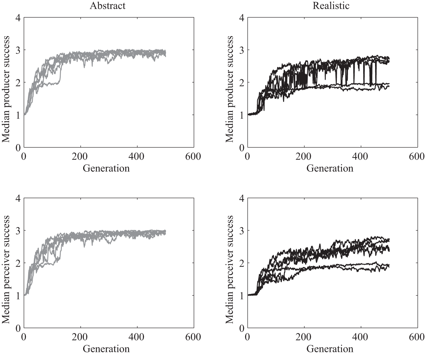
In both versions, the communicative success of the model increased as a function of generation (Figures 2 and 3). A communicative success of 3 corresponds to success on all three signals, a communicative success of 2 corresponds to success on two out of three signals, and so on. For all of the abstract-signal simulations, by about 100 generations median communicative success for both signalers and receivers was about 2.5 or greater. For the realistic-signal (embodied) simulations, some of the simulations rose quickly to that same level of performance, while others lagged behind the abstract-signal simulations, taking longer to rise to median communicative success of 2.5. Note that in simulations in which there is no selection, that is, in which agents reproduce at random, no successful signaling system evolves, since there is no selection pressure for the receivers’ and the producers’ genomes to be coordinated.

Figure 2.

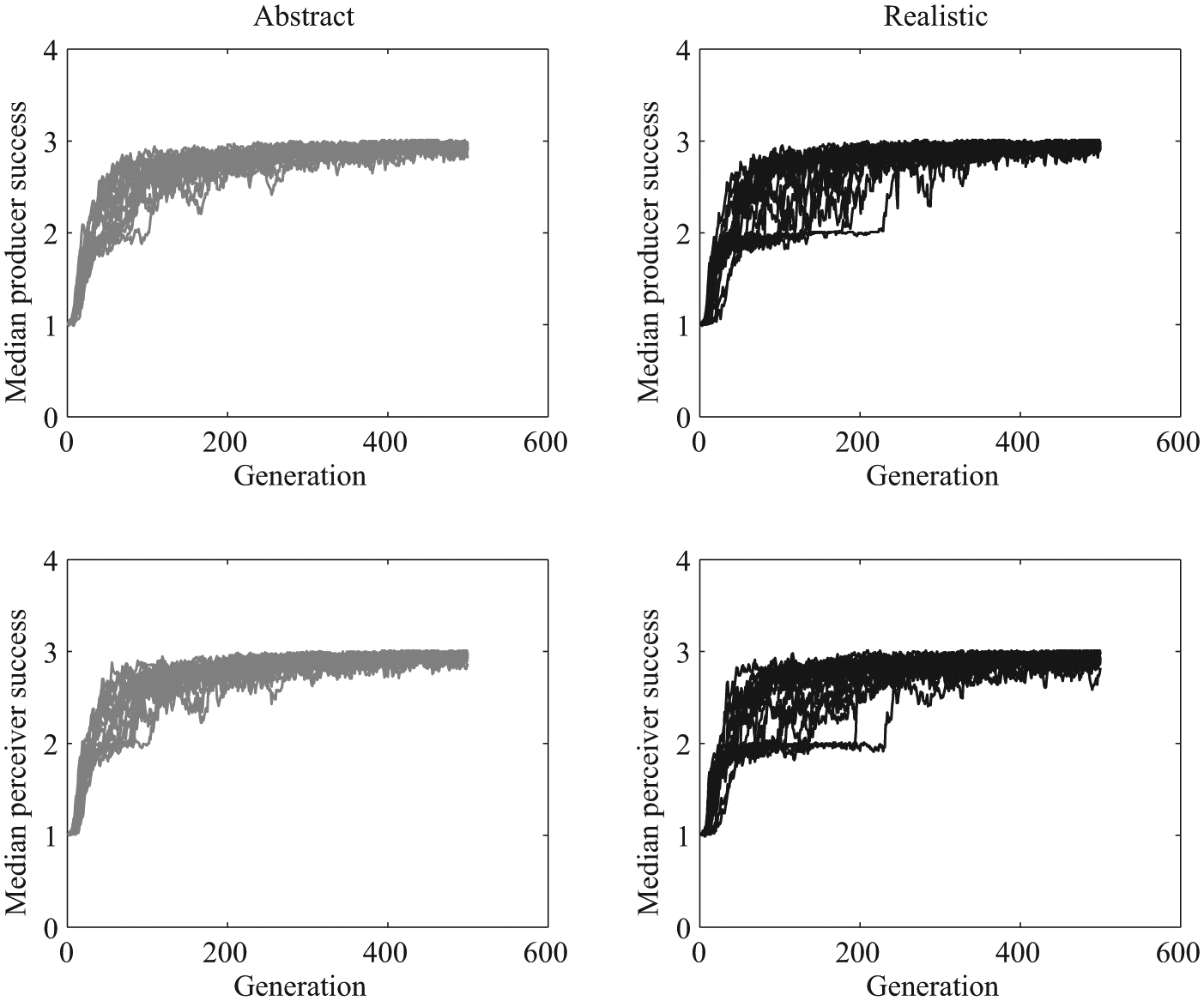
Communicative success as a function of generation. The top left panel shows each abstract simulation’s median signaler communicative success. The bottom left panel shows each abstract simulation’s median receiver communicative success. The right two panels show the signaler and receiver communicative success scores for the realistic model.

Figure 3.

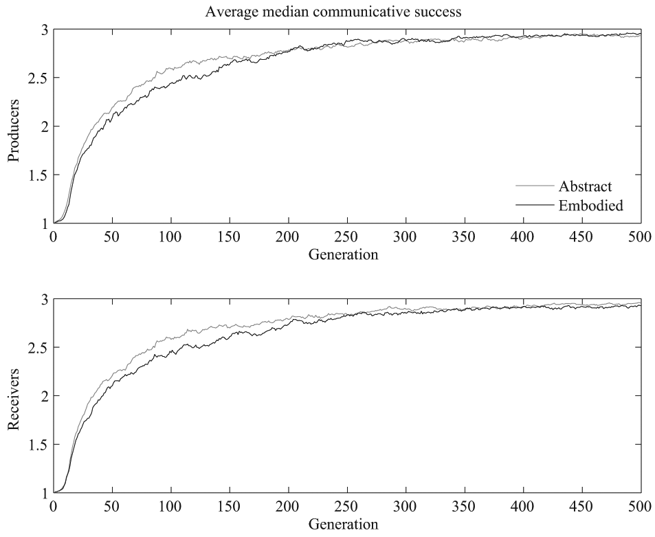
Average median communicative success across the 20 simulations of each model version. The top plot shows the average median communicative success for the producers and the bottom shows the same for the receivers.

We ran a linear mixed effects model over the median communicative success for generations 50 to 100 with simulation as a random effect and model type, generation, and interaction between model type and generation as fixed effects. Communicative success and generation were standardized prior to running the analyses. The generations were restricted to the 50–100 range in order to focus on the time point of maximal growth in communicative success, which was where differences across the two versions emerged, and in order to focus on a region of the data where trends were relatively linear and residuals approximately normally distributed. There was a statistically significant effect of generation, with communicative success increasing as generation increased, with β = 2.72 and p <.001 for the producers and β = 2.74 and p <.001 for the receivers. There was also a statistically significant effect of model version, such that overall communicative success during this time period was lower for the realistic simulations, β = −0.82 and p =.002 for the producers and β = −0.93 and p <.001 for the receivers. Additionally, there was a statistically significant interaction term for both the median producer communicative success, β = −0.43, p =.001, and the median receiver communicative success, β = −0.53, p <.001, such that the realistic simulations’ communicative success tended to increase more slowly than the abstract simulations’. Section 3.7 discusses the idea that the nonlinear transformation from producer output to perceiver input due to the vocal apparatus alters the fitness function, creating more local minima and making for this more varied and on average slower convergence.

The variability across simulations can be seen in Figure 4, which shows the standard deviation of the median communicative success across simulations for the producers and the perceivers in the realistic and abstract models. Both models have a peak in variability across simulations early on, when the greatest adaptation is taking place, and this variability tapers off as the communicative success gradually reaches its maximum value. It can also be seen that the realistic model has greater variability across simulations for both producer and perceiver communicative success during the period from around generation 75 to around generation 250. An F test comparing the variances of the two model versions’ producer communicative success values at generation 100 supports this observation that variability is greater for the realistic version, F (19, 19) = 0.27 and p = .007 for the producers and F (19, 19) = 0.34 and p = .02 for the receivers.

Figure 4.

Standard deviation of the median communicative success across the 20 simulations, which indicates variability across different evolutionary trajectories. The top plot shows the variability in the average producer communicative success across different simulations and the bottom shows the variability in the average receiver communicative success across different simulations.

In summary, it appears that robust signaling and receiving evolved at a more consistent, relatively fast rate in the abstract signal version than in the realistic signal version, in which communication sometimes evolved quickly and sometimes quite a bit more slowly.

3.2 The evolved signals

3.2.1 Comparison between realistic and abstract model signals

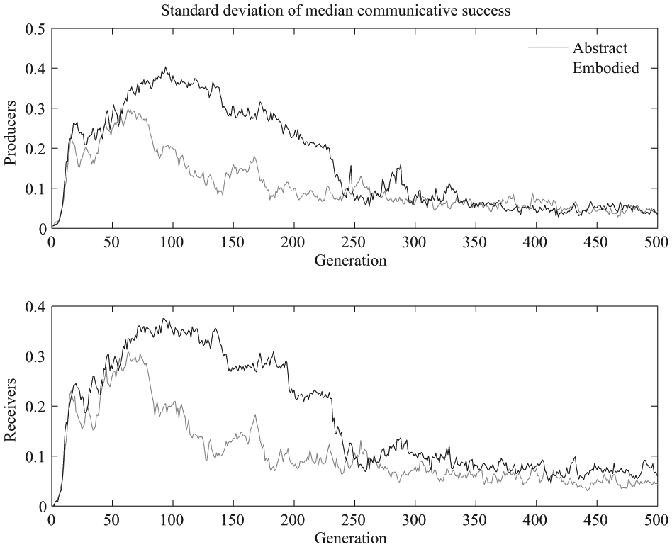
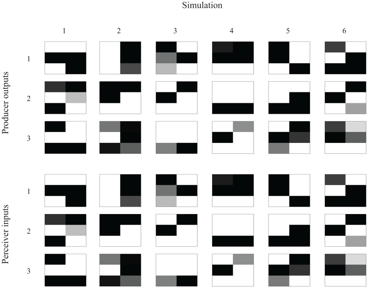
Figure 5 shows examples of the signaler outputs and the receiver inputs after 500 generations for the abstract model. The examples are from the first six of the abstract model simulations and are from the 50th most fit producer (i.e. the median producer) within each simulation. Note that for the abstract-signal model, signaler outputs and receiver inputs are the same by design.

Figure 5.

Examples of abstract model signals at generation 500. Top: the outputs produced by the median fitness producer in response to the three intended function inputs for the first six simulations of the abstract version (to save space, the other 14 simulations are not shown). Functions are in rows and simulations are in columns. Bottom: the signals, that is, the inputs given to the receivers, corresponding to each of the producer outputs shown above. Note that since these are from the abstract version of the model, the top and the bottom portions of this figure are exactly the same (compare to Figure 6). Although each signal is depicted as a three-row, two-column matrix, as far as the model was concerned the signals’ six vector elements did not have any spatial organization. Darker pixels indicate higher values.

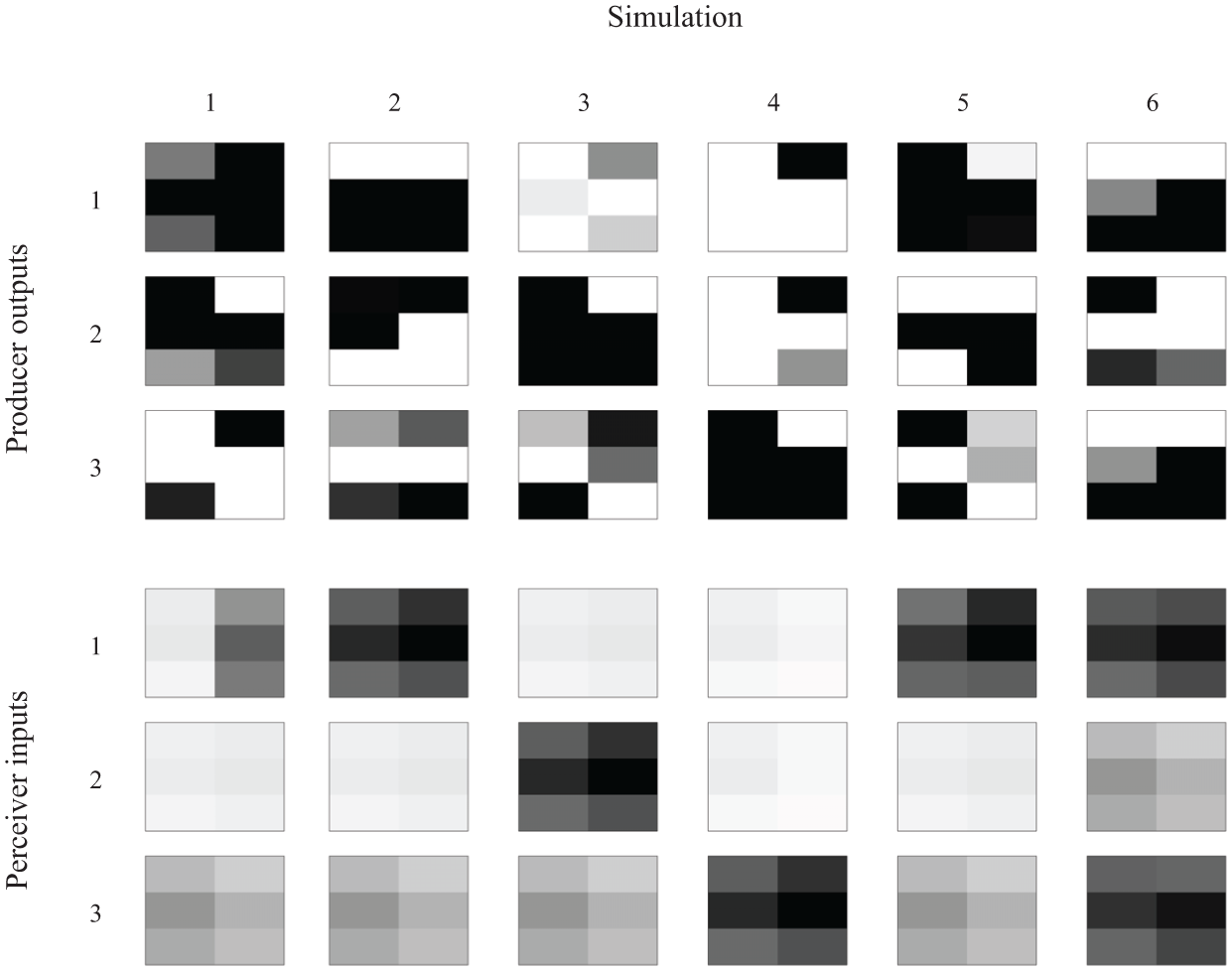
Figure 6 shows realistic model signaler outputs, which correspond to muscle activations, and receiver inputs, which correspond to the spectrograms of the sound wave resulting from those vocal tract muscle activations. Recall that these spectrograms were low-resolution mel-scaled spectrograms of actual synthesized sounds. The sounds themselves are shown in raw and in higher-resolution spectrogram forms in Figure 7. The audio files corresponding to each of the sounds in Figure 6 can be downloaded from http://dx.doi.org/10.6084/m9.figshare.1195957.

Figure 6.

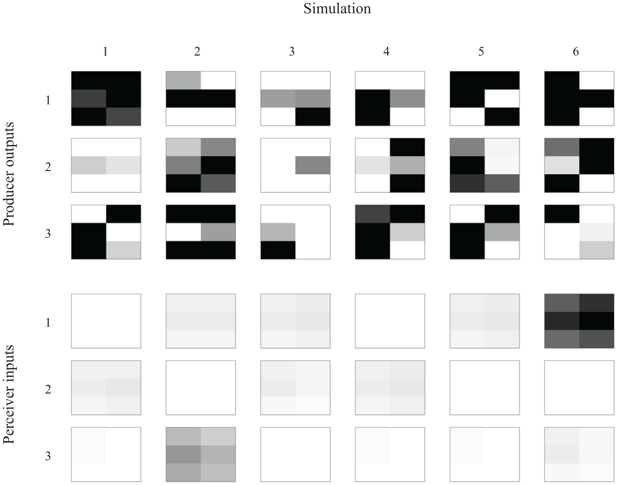
Examples of realistic model signals at generation 500. Top: the outputs produced by the median fitness producer in response to the three intended function inputs for the first six simulations of the realistic version (to save space, the other 14 simulations are not shown). Functions are in rows and simulations are in columns. Bottom: the signals, that is, the inputs given to the receivers, corresponding to each of the producer outputs shown above. In the realistic model, the producer outputs were treated as laryngeal muscle activations. These were fed into the vocal tract simulation and an acoustic signal was synthesized. This acoustic signal was then converted to a very low-resolution (two time bins and three frequency bins) spectrogram and these spectrograms were given to the receivers as input. Therefore, in the top plots the spatial matrix depiction does not have any significance while in the bottom plots the spatial layout does have meaning: the rows correspond to different frequency bins within the 20–2000 Hz range and the columns correspond to time bins within the 0.0–0.5 s range. In the bottom plots, the acoustic powers have been exponentially scaled by a power of 1/4 to make the differences between the quiet sounds more visible (future simulations might try using the log of the acoustic powers to avoid this issue). Darker pixels indicate higher values. Audio files are available at http://dx.doi.org/10.6084/m9.figshare.1195957.

Figure 7.

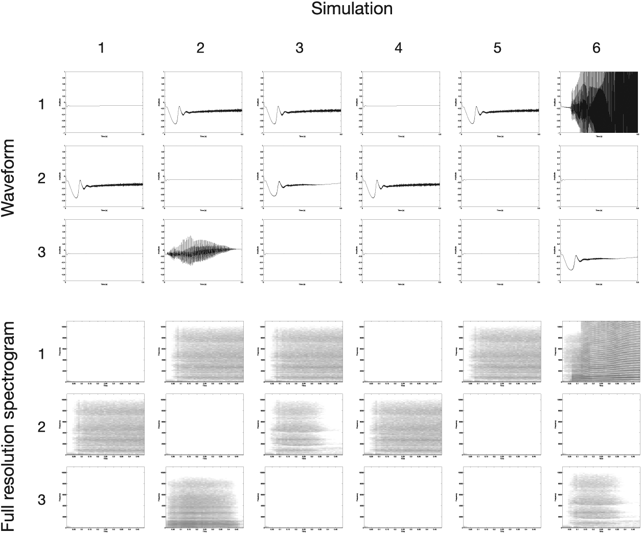
Examples of the audio signals generated by the realistic model, prior to conversion into the low-resolution spectrograms that were given as input to the receivers (see the bottom part of Figure 6). The signals are the same as those shown in Figure 6. The top half of the figure shows each signal’s raw waveform. The bottom half shows high-resolution spectrograms (not mel-scaled). In the spectrograms, darker colors indicate higher values.

When abstract signals were used, the evolved signal vectors ended up having element values that were often either all minimal (0) or maximal (1). Which vector elements were minimal or maximal for a given signal appeared to be arbitrary although within a simulation the vectors representing the three different signals were always rather different, as one would expect.

In the embodied, realistic-signal version of the model, the evolved muscle activations associated with each signal tended to have rather extreme values, as was the case in the abstract-signal version. We will discuss some possible reasons for this in the following section. The acoustics of the vocalizations resulting from these muscle activations, on the other hand, reveal that the signals that had to be categorized by the perceivers were quite different from those in the abstract-signal version (see the bottom panels of Figures 5 and 6). Most signals were very quiet and quite similar to one another, although a few of the evolved signals were louder (e.g. signal 3 in simulation 2 and signal 1 in simulation 6). Additionally, there was interdependence among elements of the signal vectors, such that when a pixel of the vocalization spectrogram was darker, nearby pixels also tended to be darker. Thus, compared to the abstract signals, there were striking differences in the signals created by transforming muscle activations to acoustic spectrograms via the vocal tract model, and this had effects on the types of signals on which the populations converged.

One way to relate the differences in the types of signals used by the realistic model to the differences observed in their performance (see Section 3.1) is to calculate the within- and between-meaning distances between signals produced by the population at the end of the simulation (i.e. at generation 500). The average pairwise distance within a simulation between the signals (i.e. the vectors that were input to the receivers) that were produced in response to different meanings was 1.77 for the abstract simulations and 0.14 for the realistic simulations. This difference was statistically significant, t(22.59) = 26.39, p <.001. The average pairwise distance between signals within a meaning category was 0.55 for the abstract simulations and 0.05 for the realistic simulations, which also was statistically significant, t(23.69) = 13.11, p <.001. We also compared the average ratio of within-simulation average within-meaning distance to within-simulation average between-meaning distance. A smaller ratio is an indication that signals corresponding to different meanings are easier to distinguish from each other within that simulation. This ratio was 0.32 for the abstract simulations and 0.68 for the realistic simulations, a difference that was also statistically significant, t(21.87) = −4.41, p <.001. The higher within- to between-meaning distance ratio and lower across-signal differences in general may be a reason for the extra challenge faced by the realistic version, reflected in the realistic model’s slower-on-average growth in communicative success over the course of the evolutionary simulations.

We also ran a cluster analysis on all the signals (i.e. the receiver inputs) produced within a simulation at generation 500. We used the mclust function from the mclust R package (Fraley, Raftery, Murphy, & Scrucca, 2012) and compared the number of clusters it estimated within a simulation for the realistic model to the number of clusters estimated for the abstract model. Mclust treats the data as a Gaussian mixture model and uses the Bayesian information criterion (BIC) to optimize the number of clusters. The maximum number of clusters was set to the default of 20. On average, 9.3 clusters were identified among the realistic model signals and on average 14.35 clusters were identified among the abstract model signals. This difference was statistically significant, t(35.49) = 2.21, p = .03. The smaller number of clusters found for the realistic model are another indication that there is reduced variation within a simulation in the types of signals that are produced when a realistic sound production mechanism is used.

3.3 Signals and genes before versus after evolution

Figures 8 and 9 show examples of the producer outputs and receiver inputs at generation 1, prior to any evolutionary adaptation taking place, when neural connection weights were random. The producer outputs tended to have less extreme values at generation 1 compared to generation 500 (Figures 5 and 6). Since the abstract model’s receiver inputs were the same as its producer outputs, the tendency toward extreme values as evolution progressed also applied to the receiver inputs in that version.

Figure 8.

Examples of individual abstract model signals at generation 1 (i.e. before any evolutionary change). Top: the outputs produced by the median fitness (i.e. the 50th most communicatively successful) producer in response to the three intended function inputs for the first six simulations of the abstract version. Bottom: the signals, that is, the inputs given to the receivers, corresponding to each of the producer outputs shown above. Compare to Figure 5. Darker pixels indicate higher values.

Figure 9.

Examples of realistic model signals at generation 1 (i.e. before any evolutionary change). Top: the outputs produced by the median fitness producer in response to the three intended function inputs for the first six simulations of the realistic version. Bottom: the signals, that is, the inputs given to the receivers, corresponding to each of the producer outputs shown above. Compare to Figure 6. Darker pixels indicate higher values.

The realistic model signals that were input to the receivers showed a different and interesting pattern. Prior to any adaptation taking place, the realistic model signals were fairly evenly split between high-amplitude, low-amplitude, and silent sounds (Figure 9). After 500 generations, the signals were predominantly silent and low-amplitude, with fewer high-amplitude sounds. This might reflect difference in the robustness of the system for generating quiet versus loud signals, with louder signals being more specific in terms of the parameters needed to produce them, and therefore more evolutionarily fragile. It is possible that additional pressures, such as a noisy environment, larger signal repertoires, or considerations of what types of signals are naturally most salient to mammalian auditory systems (Owren & Rendall, 2001) might be needed for loud signals to be maintained over the generations.

3.4 Adding environmental noise

To follow up on the issue of realistic model signals getting quieter over the course of evolution, we ran two sets of six realistic and abstract model simulations in which noise was added to each signal just prior to inputting it to each receiver. The noise consisted of six values (one corresponding to each perceiver input) drawn at random from a uniform distribution between 0 and 0.01. This did indeed result in the realistic model signals consistently having louder signal at generation 500 (See Figures 10 and 11). Interestingly, although the range of sounds produced by the realistic model was still restricted to a few types (bottom part of Figure 11), it appears that these signals could be generated via a variety of muscle activation patterns (top part of Figure 11). The addition of the noise also caused the realistic model’s communicative success to increase more slowly for both models and to have more variable and overall lower communicative success at generation 500. This was not the case for the abstract model (Figure 12). Overall, the experiment shows that the addition of noise can indeed result in added selection pressure for loud sounds to be included in the repertoire. The audio files corresponding to each of the sounds in Figure 11 can be downloaded from http://dx.doi.org/10.6084/m9.figshare.1373913.

Figure 10.

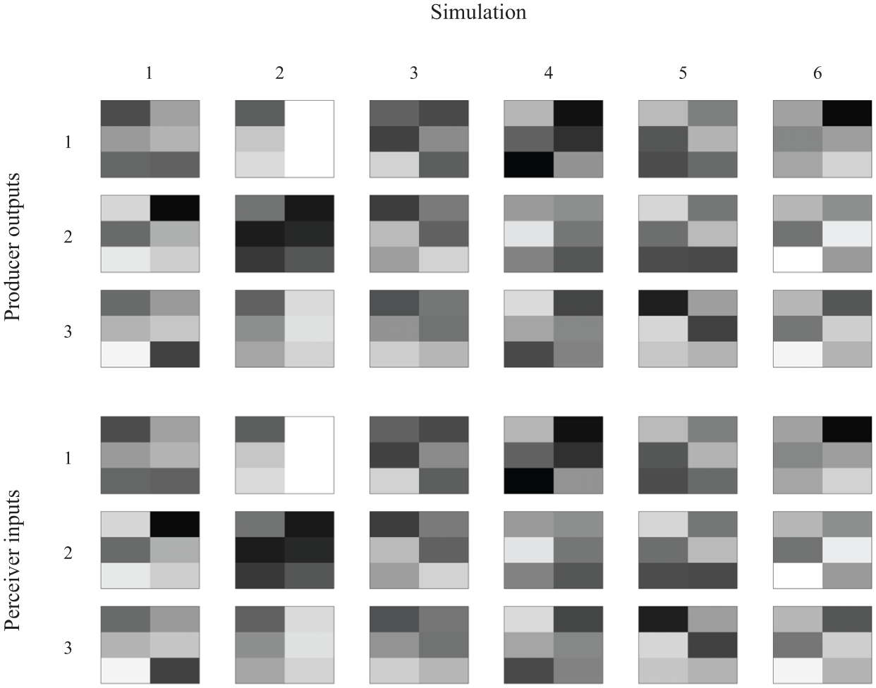
Examples of abstract model signals evolved in a noisy environment at generation 500. Top: the outputs produced by the median fitness producer in response to the three intended function inputs for the first six simulations of the realistic version. Bottom: the signals, that is, the inputs given to the receivers, corresponding to each of the producer outputs shown above. Darker pixels indicate higher values.

Figure 11.

Examples of realistic model signals evolved in a noisy environment at generation 500. Top: the outputs produced by the median fitness producer in response to the three intended function inputs for the first six simulations of the realistic version. Bottom: the signals, that is, the inputs given to the receivers, corresponding to each of the producer outputs shown above. Note the larger number of loud signals compared to Figure 6. Darker pixels indicate higher values. The corresponding audio files are available at http://dx.doi.org/10.6084/m9.figshare.1373913.

Figure 12.

Communicative success as a function of generation in simulations in which random noise was added before inputting signals to the receivers. The top left panel shows each abstract simulation’s median signaler communicative success. The bottom left panel shows each abstract simulation’s median receiver communicative success. The right two panels show the signaler and receiver communicative success scores for the realistic model. Compare to Figure 2.

3.5 Gene changes over time

The increase in extremity of weights over evolutionary time is a reflection of genetic drift over time. As evolution proceeds, the genomes tend to drift toward more and more extreme gene values, as shown in Figure 13. A follow-up experiment to test this idea confirmed that if weights are restricted to the initial range of possible values, the genomes and the producer outputs no longer show the same drift toward more extreme values over time. This is naturally reflected in the producers’ outputs. Five abstract and five realistic model simulations where weights were restricted to always remain between −1 and 1 showed very similar patterns to those reported above, when weights were unbounded. One difference was that the realistic model simulations showed greater variability in their pattern of change in communicative success over generations and showed on average slower increase in communicative success. The realistic model’s acoustic signals were similar to those reported above as were the abstract signals except that the abstract signals were not as extreme in value. Note also that in simulations in which there is no selection, there is still a tendency to drift toward more extreme gene values, although there is no increase in communicative success.

Figure 13.

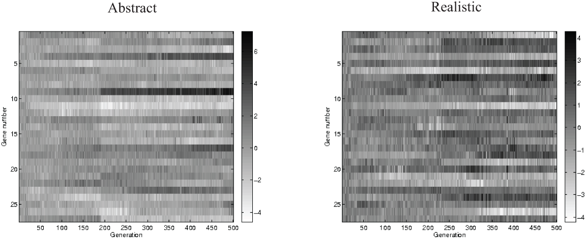
Left: the median individual’s genes plotted as a function of generation for the first simulation of the abstract model version. Right: the median individuals’ genes plotted as a function of generation for the first simulation of the realistic model version.

3.6 Muscle activations and sound loudness

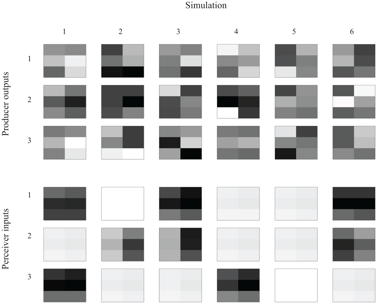
Figure 14 shows example muscle activities of each producer’s three signals for simulation 1 of the realistic version of the model without the added noise. Muscle values for signals that were relatively loud can be compared to muscle values for signals that are relatively quiet. Sounds were classified as loud versus quiet using an amplitude threshold defined as the sum of the mel frequency spectrogram (prior to reducing its resolution) being at least 0.01. Note that the muscle activations are essentially random at the beginning of the simulation, before any adaptation has taken place. Looking at the full set of muscle activations it is apparent that positive interarytenoid activation is essential for producing a relatively loud sound, but also that whether a sound is voiced does not solely depend on interarytenoid activation and is also dependent on the particular combinations of other muscles’ activities; there are sounds for which interarytenoid is positively activated but the sounds are quiet. The generation 500 muscle activities also illustrate that, in some cases, over the course of evolution the muscle activities tend to take on rather extreme values (for example, signal 1’s posterior and lateral cricoarytenoid values).

Figure 14.

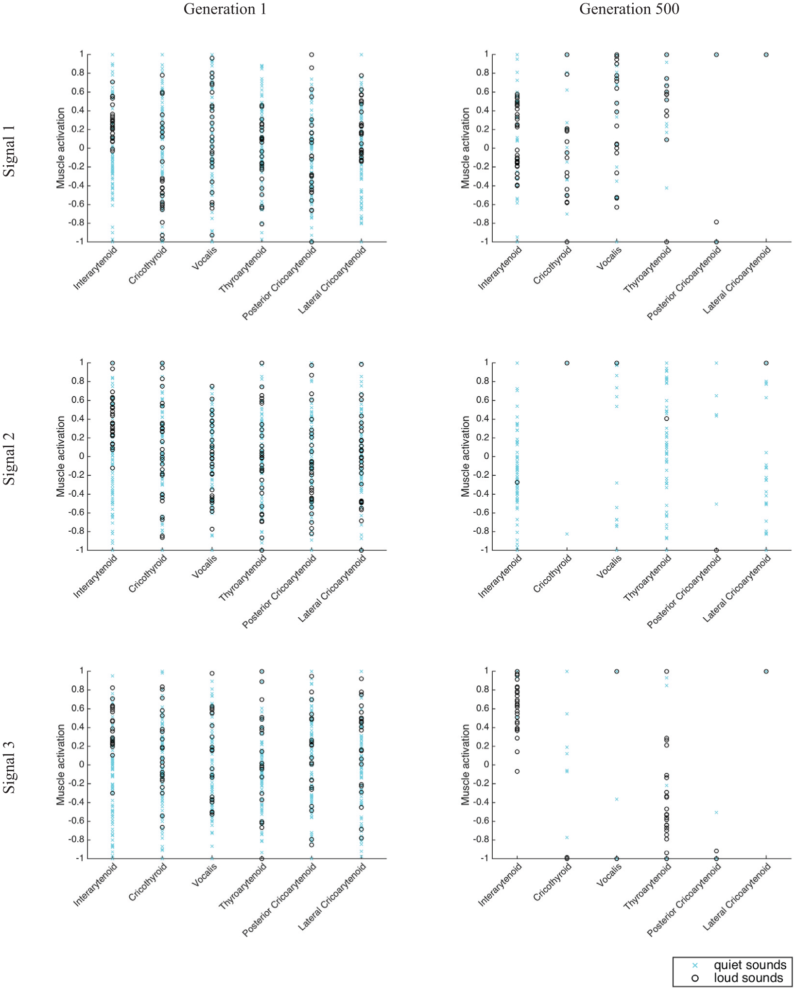
Muscle activities for each producer’s three signals for simulation 1 of the realistic version of the model with added noise. Signals from generation 1 are in the left column and signals from generation 500 are in the right column. The three signals are each displayed in different rows so that their muscle activities can be viewed as a group and compared to each other. Within each panel, each of the six muscles has its own column. Each point corresponds to the degree of activation of the given muscle for the given signal number for each of the 100 producers at the specified generation. Cyan × indicate the muscle values for sounds that are very quiet whereas black ∘ indicate the muscle values for sounds that exceeded an amplitude threshold defined as the sum of the mel frequency spectrogram being at least 0.01.

3.7 Fitness landscapes

In this section we explore the idea that the slower convergence of the realistic model is due to differences in the smoothness of the fitness landscapes across model versions (Levinthal, 1997). Since each individual has 27 genes that encode that individual’s neural network weights, the fitness landscape resides in a 27-dimensional space. It would be difficult to visualize and interpret the complete 27-dimensional fitness landscape. Instead, we systematically altered each gene individually while leaving others at their original values, then assessed the effect this alteration had on the individual’s performance. We chose to focus on the median-performing individual at generation 500. In the production case this corresponds to the individuals whose signals are shown in Figures 5 and 6. We tested four different changes to gene values: −5/7, −2.5/7, 2.5/7, and 5/7. These values were chosen to match the range of mutations actually used in the simulations, which were random increments or decrements between −5/7 and 5/7 (see Section 2.5).

Figure 15 shows the results of these tests, providing an approximation of the fitness landscapes across simulations. Darker colors in the figure indicate increases in fitness (which is proportional to communicative success) and lighter colors indicate decreases in fitness. Medium gray indicates no change in fitness. The first observation we can make is that as the genes are changed, no change and decrease in fitness (i.e. communicative success) are far more common than increase in fitness. This reflects the fact that the simulations had by generation 500 evolved to at least locally maximal communicative success.

Figure 15.

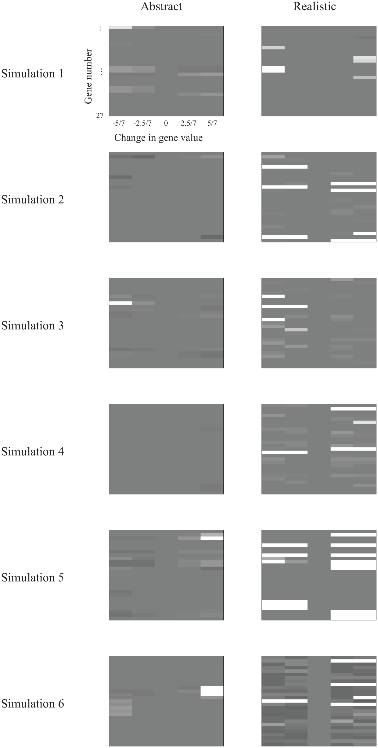
Producer fitness landscapes for the abstract (left) and realistic (right) versions of the model. See text for details on how the landscapes were created. Black indicates a fitness increase of 0.5 and white indicates a fitness decrease of 0.5. Medium gray indicates no fitness change. The middle column of each fitness landscape shows this no-change baseline. For brevity, only the first six of the 20 simulations of each version are shown.

The other observation that can be made about Figure 15 is that the realistic version of the model, shown on the right side of the figure, showed more raggedness in the fitness landscapes. In other words, small changes in individual genes were more likely to lead to substantial differences in fitness for the realistic version of the model than for the abstract version. Using a realistic signaling apparatus, that is, a humanoid vocal tract model, made for rougher fitness landscapes, at least in the space surrounding the end state solution. The introduction of a body increases the complexity of the communication evolution problem. This should have implications for the neural circuitry required to support a system of multiple distinct and stable vocal signal types.

4 Discussion

We compared two versions of a computational model of vocal signal evolution, one that used abstract signals, similar to previous models, and one in which signals were synthesized through simulation of a human vocal tract. Both model versions converged to a near optimum state where the individual successfully communicated all three signals. There were differences, however, in the number of generations it took to converge to this near-optimal state, in the signals that ended up being converged upon, and in the ruggedness of the fitness landscapes. On average, the embodied, realistic-signal model improved in performance more slowly than the abstract model. The realistic version also exhibited more variable rates of adaptation across simulations.

The realistic model evolved signals that had characteristics very different to those of the abstract signals. First of all, the signal elements input to the receivers were not independent from one another. When one spectrogram pixel increased in amplitude, the others tended to as well. In contrast, the values of the elements of the abstract model signals could vary more independently from each other. Second, and related to the first point, the realistic model’s three signals tended to be more similar to each other, as measured in terms of both intra- and inter-signal variability. Third, the ratio of intra- to inter-signal variability was higher for the realistic model, which indicates a lower degree of signal separation in the realistic model and illustrates the challenges faced by the realistic version compared to the abstract version, possibly explaining why the realistic version on average took more time to adapt. Estimations of the fitness landscapes showed rougher landscapes for the realistic model version, further supporting the idea that the constraint of evolving signals using a realistic vocal tract makes the adaptation process as well as the resulting signals less robust. The slower average rate of convergence is also consistent with this idea.

These results suggest that computational neural network models of vocal signal evolution remain capable of evolving multiple distinct signals when subjected to physiological and physical constraints imposed by the primate vocal tract and the acoustic modality. At the same time, embodiment in a more physiologically realistic signaling system can affect both the rate and outcome of signal evolution, and the physiological and physical constraints create, at least in the present case, a fitness landscape that is more rugged than the fitness landscape for a model with purely abstract signals. This reflects the fact that the process of phonation, on which most primate vocal signals rely, involves a complex and nonlinear relationship between motor actions and resulting sound, as was observed upon examining the realistic model’s muscle activations in comparison to the signals’ acoustic amplitude (Fletcher, 1996). The signalers and receivers can be seen as evolving interpersonal synergies (Riley, Richardson, Shockley, & Ramenzoni, 2011) in which the degrees of freedom of the two groups of individuals become coupled in ways that respect the nonlinearities of the motor and sensory systems and of the mechanics and acoustics of the vocal tract. The differences we observed between the realistic version and the abstract version justify increased attention to physiological and modality-specific factors in models of communication evolution (see Turvey, 1990, for a more general argument in favor of considering the relationship between the motor system and the physical world when studying motor control).

An obvious advantage of using a realistic vocal tract is that all the resulting signals are similar to sounds that humans do indeed produce. The actual sounds that the realistic model converged upon were only semi-realistic in terms of representing the types of reflexive signals humans can make. Within a simulation, one of the model’s signals was always a silent sound (Figures 6 and 7). Another signal was usually a breathy sound. The third signal tended to either be a slight variant of the first two sounds or was a much louder sound, similar to a moan. Interestingly, the tendency for two of the signals to often be close variants of each other may be quite realistic, as it is known that non-human primate vocal calls exhibit continuous gradations (Oller & Griebel, 2014; Price, 2013). The present study thus indicates that continuously varying call types could potentially result from genetic adaptation of neural control of the vocal tract even when the functions being served by the signals are completely distinct and independent. When noise was added, the range of types of signals in the repertoire did not change, but the signals were more likely to include at least one or two of these louder moaning sounds. However, when noise was added, the number of signals that the realistic model successfully evolved was sometimes lower than when there was no noise; this was not the case for the abstract model with noise simulations (see Nowak & Krakauer, 1999, for more on how noise can reduce the number of signals in a repertoire). The fact that the addition of environmental noise adds sensitivity to the realistic model’s evolution further exemplifies the potential interactions that may occur between bodies, neural circuitry, and environment. The abstract modeling approach cannot account for these realistic interactions.

The model was simplified to have a maximum of three signals and to involve only static manipulations of laryngeal muscles with no change over time in muscle activation, and with all lung and upper vocal tract muscles remaining constant across all sounds. These simplifications certainly restricted the extent to which the model could possibly converge on a full primate-like repertoire of vocal calls. Future work could presumably improve on this limitation by lifting these restrictions. One feature of primate vocalizations that is not addressed by our model is their sequential organization, including both within-signal temporal variation and variation in sequencing of signals (Arnold & Zuberbühler, 2006; Simmons & McRae, 2014). Recurrent neural network architectures may allow future work to address the emergence of primate-like signals that involve temporal sequences (Di Paolo, 2000; Ryan et al., 2001; Seys & Beer, 2004; Werner & Dyer, 1992).

Future work should explore additional variations on these models, for example varying the population size, number of signals to be communicated, perceptual encoding of the signals (such as log-transforming the energies in the spectrograms, changing the frequency ranges represented, and changing the resolution of the spectrograms), and genetic algorithm parameters. Alternative neural network architectures and genetic encodings should also be explored. Different modes of genetic encoding of neural network properties, such as aspects of neuronal development, will be particularly important in future work since direct encoding of neural weights within the genome is not biologically realistic and is also unlikely to scale up to larger neural network models (Cangelosi, Parisi, & Nolfi, 1994; Stanley & Miikkulainen, 2003; Werner & Dyer, 1992).

The finding that realistic physiological and physical constraints affected the kinds of signals that evolved is consistent with the idea that differences in the vocal and auditory apparatus across species are partly responsible for differences in their evolved signals. This is supported by Negus’s findings (as cited in Ploog, 1992) that human larynges are more specialized for phonation than those of canids, which are more specialized for phonation than those of animals like horses. Computational modeling of different vocal tract configurations also provides support for the importance of variations in vocal tract shape (De Boer, 2010, 2012). The evolution of the vocal tract and the evolution of neural circuitry for controlling that vocal tract should in the future be addressed in combination, as has been done in some other domains of evolutionary simulation (Chiel & Beer, 1997; Sims, 1995). A related issue worth exploring is how communicative vocal signals may have evolved from non-communicative functions of the vocal tract (Davis & MacNeilage, 1995; Goldstein, Byrd, & Saltzman, 2006; MacNeilage, 1998; Nolfi, 2005). For example, the larynx plays a role both in breath control and in phonation, with the former being phylogenetically older. The present work supports the role of the embodied production mechanism in shaping the evolution of neural controllers and perceivers; an important next step is to study the evolution of neural controllers serving different functions, for example one communicative and one related to breathing or feeding, but making use of the same bodily structures.

As noted Section 1, the majority of work on human vocal adaption has focused on vocal learning, specifically on learning to produce and perceive speech sounds. One future goal is to combine modeling of the evolution of vocal signals with modeling of vocal learning (see also Ackley & Littman, 1992; Batali, 1994; MacLennan & Burghardt, 1994; Nolfi, 2005; Nolfi & Floreano, 1999; Smith, 2002; Werner & Dyer, 1992). There is evidence that while reflexive primate vocalizations share many acoustic features across infant and adult productions, in some cases learning shapes the form of the calls over the course of development (Seyfarth & Cheney, 1986). Furthermore, it has been proposed that motor control for speech production draws on neural networks in the limbic system and brainstem that are used to generate reflexive vocalizations as well as other reflexes involving vocal tract structures (Barlow et al., 2009; Barlow, Farley, & Andreatta, 1999; Deacon, 1989; Ghazanfar & Takahashi, 2014; Ghazanfar et al., 2012; Grillner, 1982; Jürgens, 2002; Schulz et al., 2005). It therefore makes good sense to build models of reflexive signal production as well as of speech production that incorporate more ancient evolved vocal networks as well as the capability to learn to utilize them in the service of producing novel sounds. Building models of the evolution of neural circuits that produce reflexive signals such as cries, laughs, screams, moans, and lip smacks is a prerequisite for this more comprehensive modeling of human vocalization that takes into account both reflexive signals and speech. The present work represents an initial step in this direction. Including learning on the part of the perceivers is also important (Nolfi, 2005), especially in the case of vocal signaling given that while the vocal productions of non-human primates are relatively fixed, their capacity for perceptual learning of responses to communicative signals appears much greater (Owren & Rendall, 2001).

Finally, producing and perceiving communicative signals using biologically realistic effectors and sensors is only one aspect of embodiment (Chiel & Beer, 1997; Pezzulo et al., 2011). Many other features of the world and body are relevant to the evolution of communication systems. For example, having to act with a physical body comprised of arms, legs, and so on, and having to interact with the world, including other agents, using vision, touch, and other modalities, are aspects of embodiment that have been considered in previous models of the evolution of communication abilities (Cangelosi & Parisi, 2001; Parisi, 1997; Steels & Vogt, 1997). These other aspects of embodiment are also important in understanding the conditions under which human communication may have evolved and under which it develops. Furthermore, other parts of the body and the environment can affect the way in which sounds are perceived and produced, for example by attenuating the amplitude of sounds in ways that can affect the signaling systems which evolve (Di Paolo, 2000). The energetic cost of signal production might also be an important factor (Levin, 1995; Oudeyer, 2005). Additionally, the functions served by a signal have been previously shown to co-evolve in interesting ways with the form of a signal (Di Paolo, 2000; Marocco & Nolfi, 2007; Quinn et al., 2003); how this will be affected by the use of biologically realistic sound production mechanisms is a topic for future study. Ultimately, it would be worthwhile to create models of embodied communication emergence that take into consideration the many facets of embodiment and their interaction with one another, including the physical generation of sound by the body (Nolfi, 2005).

Footnotes

Funding

Early stages of this work were supported by a United States Department of Energy Computational Science Graduate Fellowship (DE-FG02-97ER25308).

About the Authors

Anne S Warlaumont is currently an assistant professor of cognitive and information sciences at the University of California, Merced, CA. In 2012 she received her PhD in communication sciences and disorders with a certificate in cognitive science from the University of Memphis. In 2006 she received her BA in psychology with a cognitive science concentration from Cornell University. Her research focuses on the development and evolution of human vocal communication, building artificial neural networks that control simulated vocal tracts and analyzing naturalistic audio recordings of human infants.

Andrew M Olney presently serves as associate professor in both the institute for intelligent systems and department of psychology and as director of the institute for intelligent systems at the University of Memphis. Olney received a BA in linguistics with cognitive science from University College London in 1998, an MS in evolutionary and adaptive systems from the University of Sussex in 2001, and a PhD in computer science from the University of Memphis in 2006. His primary research interests are in natural language interfaces. Specific interests include vector space models, dialogue systems, unsupervised grammar induction, robotics, and intelligent tutoring systems.

References

Ackley

Littman

(1992). Interactions between learning and evolution. In Langton

C. G.

Taylor

Farmer

J. D.

Rasmussen

(Eds.), Artificial life II (pp. 487–509). Redwood City, CA: Addison-Wesley Publishing Company.

Arnold

Pohlner

Zuberbühler

(2008). A forest monkey’s alarm call series to predator models. Behavioral Ecology and Sociobiology, 62(4), 549–559.

Arnold

Zuberbühler

(2006). Language evolution: Semantic combinations in primate calls. Nature, 441(7091), 303–303.

Barlow

S. M.

Farley

G. R.

Andreatta

R. D.

(1999). Neural systems in speech physiology. In Barlow

S. M.

Andreatta

R. D.

(Eds.), Handbook of clinical speech physiology (pp. 101–163). San Diego, CA: Singular Publishing Group.

Barlow

S. M.

Lund

J. P.

Estep

Kolta

(2009). Central pattern generators for orofacial movements and speech. In Brudzynski

S. M.

(Ed.), Handbook of mammalian vocalization: An integrative neuroscience approach (pp. 351–369). New York, NY: Academic Press.

Bass

A. H.

Remage-Healey

(2008). Central pattern generators for social vocalization: Androgen-dependent neurophysiological mechanisms. Hormones and Behavior, 53(5), 659–672.

Batali

(1994). Innate biases and critical periods: Combining evolution and learning in the acquisition of syntax. In Brooks

Maes

(Eds.), Artificial life IV (pp. 160–171). Cambridge, MA: MIT Press.

Benz

J. J.

(1993). Food-elicited vocalizations in golden lion tamarins: Design features for representational communication. Animal Behaviour, 45(3), 443–455.

Biben

Symmes

Masataka

(1986). Temporal and structural analysis of affiliative vocal exchanges in squirrel monkeys (Saimiri sciureus). Behaviour, 98(1), 259–273.

10.

Bocchi

Lapi

Ballerini

(2010). Evolution of communicating individuals. In Chio

Cagnoni

Cotta

Ebner

Ekárt

Esparcia-Alcazar

A. I.

Yannakakis

… G. N.

(Eds.), Applications of evolutionary computation (Vol. 6024, pp. 328–335). Berlin, Germany: Springer Berlin Heidelberg.

11.

Boersma

(1998). Functional phonology: Formalizing the interactions between articulatory and perceptual drives. The Hague, The Netherlands: Holland Academic Graphics.

12.

Boersma

Weenink

(2010). Praat: Doing phonetics by computer (version 5.1.31). Computer software. Retrieved from http://www.fon.hum.uva.nl/praat/

13.

Bryant

G. A.

Aktipis

C. A.

(2014). The animal nature of spontaneous human laughter. Evolution and Human Behavior, 35(4), 327–335.

14.

Cangelosi

Parisi

(1998). The emergence of a ‘language’ in an evolving population of neural networks. Connection Science, 10(2), 83–97.

15.

Cangelosi

Parisi

(2001). How nouns and verbs differentially affect the behavior of artificial organisms. In Moore

J. D.

Stenning

(Eds.), Proceedings of the 23rd annual conference of the cognitive science society (pp. 170–175).

16.

Cangelosi

Parisi

Nolfi

(1994). Cell division and migration in a ‘genotype’ for neural networks. Network: Computation in Neural Systems, 5(4), 497–515.

17.

Chater

Reali

Christiansen

M. H.

(2009). Restrictions on biological adaptation in language evolution. Proceedings of the National Academy of Sciences of the United States of America, 106(4), 1015–1020.

18.

Chiel

H. J.

Beer

R. D.

(1997). The brain has a body: Adaptive behavior emerges from interactions of nervous system, body and environment. Trends in Neurosciences, 20(12), 553–557.

19.

Davis

B. L.

MacNeilage

P. F.

(1995). The articulatory basis of babbling. Journal of Speech and Hearing Research, 38(6), 1199–1211.

20.

Deacon

T. W.

(1989). The neural circuitry underlying primate calls and human language. Human Evolution, 4(5), 367–401.

21.

De Boer

(2000). Self-organization in vowel systems. Journal of Phonetics, 28(4), 441–465.

22.

De Boer

(2001). The origins of vowel systems. Oxford, UK: Oxford University Press.

23.

De Boer

(2010). Modelling vocal anatomy’s significant effect on speech. Journal of Evolutionary Psychology, 8(4), 351–366.

24.

De Boer

(2012). Loss of air sacs improved hominin speech abilities. Journal of Human Evolution, 62(1), 1–6.

25.

Delvolvé

Branchereau

Dubuc

Cabelguen

J.-M.

(1999). Fictive rhythmic motor patterns induced by NMDA in an in vitro brain stem-spinal cord preparation from an adult urodele. Journal of Neurophysiology, 82(2), 1074–1077.

26.

De Saussure

(1983). Course in general linguistics ( Harris

, Trans.) Chicago, USA: Open Court.

27.

Di Paolo

E. A.

(2000). Behavioral coordination, structural congruence and entrainment in a simulation of acoustically coupled agents. Adaptive Behavior, 8(1), 27–48.

28.

Ellis

D. P. W.

(2007). PLP and RASTA (and MFCC, and inversion) in MATLAB. Computer software. Retrieved from http://labrosa.ee.columbia.edu/matlab/rastamat/

29.

Elowson

A. M.

Tannenbaum

P. L.

Snowdon

C. T.

(1991). Food-associated calls correlate with food preferences in cotton-top tamarins. Animal Behaviour, 42(6), 931–937.

30.

Fischer

Hammerschmidt

(2010). Information and influence in animal communication. In Smith

A. D. M.

Schouwstra

Boer

B. de

Smith

(Eds.), The evolution of language (pp. 129–136). Singapore: World Scientific Publishing.

31.

Fletcher

N. H.

(1996). Nonlinearity, complexity, and control in vocal systems. In Davis

P. J.

Fletcher

N. H.

(Eds.), Vocal fold physiology: Controlling complexity and chaos (pp. 3–16). San Diego, CA: Singular Publishing Group.

32.

Fraley

Raftery

A. E.

Murphy

T. B.

Scrucca

(2012). Mclust version 4 for r: Normal mixture modeling for model-based clustering, classification, and density estimation (Technical Report number597). Department of Statistics, University of Washington, WA.

33.

Ghazanfar

A. A.

Takahashi

D. Y.

(2014). Facial expressions and the evolution of the speech rhythm. Journal of Cognitive Neuroscience, 26(6), 1196–1207.

34.

Ghazanfar

A. A.

Takahashi

D. Y.

Mathur

Fitch

W. T.

(2012). Cineradiography of monkey lip-smacking reveals putative precursors of speech dynamics. Current Biology, 22(13), 1176–1182.

35.

Goldstein

Byrd

Saltzman

(2006). The role of vocal tract gestural action units in understanding the evolution of phonology. In Arbib

M. A.

(Ed.), Action to language via the mirror neuron system (pp. 215–249). Cambridge, UK: Cambridge University Press.

36.

Grillner

(1982). Possible analogies in the control of innate motor acts and the production of sound in speech. In Grillner

Lindblom

Lubker

Persson

(Eds.), Speech motor control (pp. 217–229). Oxford, UK: Pergamon Press.

37.

Grillner

Wallen

(1985). Central pattern generators for locomotion, with special reference to vertebrates. Annual Review of Neuroscience, 8(1), 233–261.

38.

Heintz

Beckman

Fosler-Lussier

Ménard

(2009). Evaluating parameters for mapping adult vowels to imitative babbling. In Proceedings of the 10th annual conference of the international speech communication association (INTERSPEECH). Brighton, UK.

39.

Herzog

Hopf

(1984). Behavioral responses to species-specific warning calls in infant squirrel monkeys reared in social isolation. American Journal of Primatology, 7(2), 99–106.

40.

Hockett

C. F.

(1960). The origin of speech. Scientific American, 203, 89–96.

41.

Howard

I. S.

Messum

(2011). Modeling the development of pronunciation in infant speech acquisition. Motor Control, 15(1), 85–117.

42.

Ijspeert

A. J.

(2008). Central pattern generators for locomotion control in animals and robots: A review. Neural Networks, 21(4), 642–653.

43.

Ishizaka

Flanagan

J. L.

(1972). Synthesis of voiced sounds from a two-mass model of the vocal cords. Bell System Technical Journal, 51(6), 1233–1268.

44.

Jürgens

(1992). On the neurobiology of vocal communication. In Papoušek

Jürgens

Papoušek

(Eds.), Nonverbal vocal communication: Comparative and developmental approaches (pp. 31–42). Cambridge, UK: Cambridge University Press.

45.

Jürgens

(2002). Neural pathways underlying vocal control. Neuroscience and Biobehavioral Reviews, 26(2), 235–258.

46.

Kanda

Ogata

Komatani

Okuno

H. G.

(2008). Vowel imitation using vocal tract model and recurrent neural network. In Ishikawa

Doya

Miyamoto

Yamakawa

(Eds.), Lecture notes in computer science: Neural information processing (Vol. 4985, pp. 222–232). Berlin, Germany: Springer.

47.

Krakauer

D. C.

Johnstone

R. A.

(1995). The evolution of exploitation and honesty in animal communication: A model using artificial neural networks. Philosophical Transactions of the Royal Society B: Biological Sciences, 348(1325), 355–361.

48.

Kröger

B. J.

Kannampuzha

Kaufmann

(2014). Associative learning and self-organization as basic principles for simulating speech acquisition, speech production, and speech perception. EPJ Nonlinear Biomedical Physics, 2(1), 2.

49.

Kröger

B. J.

Kannampuzha

Neuschaefer-Rube

(2009). Towards a neurocomputational model of speech production and perception. Speech Communication, 51, 793–809.

50.

Levin

(1995). The evolution of understanding: A genetic algorithm model of the evolution of communication. Biosystems, 36(3), 167–178.

51.

Levinthal

D. A.

(1997). Adaptation on rugged landscapes. Management Science, 43(7), 934–950.

52.

Lieberman

(1968). Primate vocalizations and human linguistic ability. The Journal of the Acoustical Society of America, 44(6), 1574–1584.

53.

Lieberman

Harris

K. S.

Wolff

Russell

L. H.

(1971). Newborn infant cry and nonhuman primate vocalization. Journal of Speech and Hearing Research, 14(4), 718–727.

54.

MacKay-Lyons

(2002). Central pattern generation of locomotion: A review of the evidence. Physical Therapy, 82(1), 69–83.

55.

MacLennan

B. J.

Burghardt

G. M.

(1994). Synthetic ethology and the evolution of cooperative communication. Adaptive Behavior, 2(2), 161–188.

56.

MacNeilage

(1998). The frame/content theory of evolution of speech production. Behavioral and Brain Sciences, 21(4), 499–511.

57.

Marocco

Nolfi

(2007). Emergence of communication in embodied agents evolved for the ability to solve a collective navigation problem. Connection Science, 19(1), 53–74.

58.

Masataka

(1983a). Categorical responses to natural and synthesized alarm calls in Goeldi’s monkeys (Callimico goeldii). Primates, 24(1), 40–51.

59.

Masataka

(1983b). Psycholinguistic analyses of alarm calls of Japanese monkeys (Macaca fuscata fuscata). American Journal of Primatology, 5(2), 111–125.

60.

Miller

A. J.

(1972). Characteristics of the swallowing reflex induced by peripheral nerve and brain stem stimulation. Experimental Neurology, 34(2), 210–222.

61.

Mitchell

(1998). An introduction to genetic algorithms. Cambridge, MA: MIT Press.

62.

Miura

Yoshikawa

Asada

(2012). Vowel acquisition based on an auto-mirroring bias with a less imitative caregiver. Advanced Robotics, 26(1–2), 23–44.

63.

Moulin-Frier

Nguyen

S. M.

Oudeyer

P.-Y.

(2014). Self-organization of early vocal development in infants and machines: The role of intrinsic motivation. Frontiers in Cognitive Science, 4, 1006.

64.

Nam

Goldstein

L. M.

Giulivi

Levitt

A. G.

Whalen

(2013). Computational simulation of CV combination preferences in babbling. Journal of Phonetics, 41(2), 63–77.

65.

Noble

de Ruiter

J. P.

Arnold

(2010). From monkey alarm calls to human language: How simulations can fill the gap. Adaptive Behavior, 18(1), 66–82.

66.

Nolfi

(2005). Emergence of communication in embodied agents: Co-adapting communicative and non-communicative behaviours. Connection Science, 17(3–4), 231–248.

67.

Nolfi

Floreano

(1999). Learning and evolution. Autonomous Robots, 7(1), 89–113.

68.

Nowak

M. A.

Krakauer

D. C.

(1999). The evolution of language. Proceedings of the National Academy of Sciences of the United States of America, 96(14), 8028–8033.

69.

Oller

D. K.

(2000). The emergence of the speech capacity. Mahwah, NJ: Lawrence Erlbaum Associates.

70.

Oller

D. K.

Buder

E. H.

Ramsdell

H. L.

Warlaumont

A. S.

Chorna

Bakeman

(2013). Functional flexibility of infant vocalization and the emergence of language. Proceedings of the National Academy of Sciences of the United States of America, 110(16), 6318–6323.

71.

Oller

D. K.

Griebel

(2014). On quantitative comparative research in communication and language evolution. Biological Theory, 9(3), 296–308.

72.

Oudeyer

P.-Y.

(2005). How phonological structures can be culturally selected for learnability. Adaptive Behavior, 13(4), 269–280.

73.

Oudeyer

P.-Y.

(2006). Self-organization in the evolution of speech. Oxford, UK: Oxford University Press.

74.

Owren

M. J.

Bernacki

R. H.

(1988). The acoustic features of vervet monkey alarm calls. The Journal of the Acoustical Society of America, 83(5), 1927–1935.

75.

Owren

M. J.

Goldstein

M. H.

(2008). Scaffolds for babbling: Innateness and learning in the emergence of contexually flexible vocal production in human infants. In Oller

D. K.

Griebel

(Eds.), Evolution of communicative flexibility: Complexity, creativity, and adaptability in human and animal communication (pp. 169–192). Cambridge, MA: MIT Press.

76.

Owren

M. J.

Rendall

(2001). Sound on the rebound: Bringing form and function back to the forefront in understanding nonhuman primate vocal signaling. Evolutionary Anthropology: Issues, News, and Reviews, 10(2), 58–71.

77.

Parisi

(1997). An artificial life approach to language. Brain and Language, 59(1), 121–146.

78.

Pearson

K. G.

(1995). Proprioceptive regulation of locomotion. Current Opinion in Neurobiology, 5(6), 786–791.

79.

Pezzulo

Barsalou

L. W.

Cangelosi

Fischer

M. H.

McRae

Spivey

M. J.

(2011). The mechanics of embodiment: A dialog on embodiment and computational modeling. Frontiers in Psychology, 2, 5.

80.

Ploog

D. W.

(1992). The evolution of vocal communication. In Papoušek

Jürgens

Papoušek

(Eds.), Nonverbal vocal communication: Comparative and developmental approaches (pp. 6–30). Cambridge, UK: Cambridge University Press.

81.

Price

(2013). Vocal communication within the genus chlorocebus: Insights into mechanisms of call production and call perception. PhD Dissertation, Georg-August-Universität Göttingen, Göttingen, Germany.

82.

Quinn

Smith

Mayley

Husbands

(2003). Evolving controllers for a homogeneous system of physical robots: Structured cooperation with minimal sensors. Philosophical Transactions of the Royal Society A: Mathematical, Physical and Engineering Sciences, 361(1811), 2321–2343.

83.

Riley

M. A.

Richardson

M. J.

Shockley

Ramenzoni

V. C.

(2011). Interpersonal synergies. Frontiers in Psychology, 2, 38.

84.

Ryan

M. J.

Phelps

S. M.

Rand

A. S.

(2001). How evolutionary history shapes recognition mechanisms. Trends in Cognitive Sciences, 5(4), 143–148.

85.

Schulz

G. M.

Varga

Jeffires

Ludlow

C. L.

Braun

A. R.

(2005). Functional neuroanatomy of human vocalization: An h215o PET study. Cerebral Cortex, 15(12), 1847–1835.

86.

Seyfarth

R. M.

Cheney

D. L.

(1986). Vocal development in vervet monkeys. Animal Behaviour, 34(6), 1640–1658.

87.

Seyfarth

R. M.

Cheney

D. L.

Marler

(1980a). Monkey responses to three different alarm calls: Evidence of predator classification and semantic communication. Science, 210(4471), 801–803.

88.

Seyfarth

R. M.

Cheney

D. L.

Marler

(1980b). Vervet monkey alarm calls: Semantic communication in a free-ranging primate. Animal Behaviour, 28(4), 1070–1094.

89.

Seys

C. W.

Beer

R. D.

(2004). Evolving walking: The anatomy of an evolutionary search. In Schaal

Ijspeert

Billard

Vijayakumar

Hallam

Meyer

J.-A.

(Eds.), Animals to animats 8: Proceedings of the eighth international conference on simulation of adaptive behavior (pp. 357–363). Los Angeles, CA.

90.

Simmons

B. A.

McRae

T. R.

(2014). Hidden Markov models of eastern gray squirrel (Sciurus carolinensis) alarm calls. Adaptive Behavior, 22(3), 180–188.

91.

Sims

(1995). Evolving 3D morphology and behavior by competition. Artificial Life, 1(4), 353–372.

92.

Smith

(2002). Natural selection and cultural selection in the evolution of communication. Adaptive Behavior, 10(1), 25–45.

93.

Snowdon

C. T.

Pola

Y. V.

(1978). Interspecific and intraspecific responses to synthesized pygmy marmoset vocalizations. Animal Behaviour, 26, 192–206.

94.

Stanley

K. O.

Miikkulainen

(2003). A taxonomy for artificial embryogeny. Artificial Life, 9(2), 93–130.

95.

Steels

Vogt

(1997). Grounding adaptive language games in robotic agents. In Husband

Harvey

(Eds.), Proceedings of the 4th European conference on artificial life. Cambridge, MA: MIT Press.

96.

Talmage-Riggs

Winter

Ploog

Mayer

(1972). Effect of deafening on the vocal behavior of the squirrel monkey. Folia Primatologica, 17(5–6), 404–420.

97.

Turvey

M. T.

(1990). Coordination. American Psychologist, 45(8), 938–953.

98.

Wagner

Reggia

J. A.

Uriagereka

Wilkinson

G. S.

(2003). Progress in the simulation of emergent communication and language. Adaptive Behavior, 11(1), 37–69.

99.

Warlaumont

A. S.

(2013). Salience-based reinforcement of a spiking neural network leads to increased syllable production. In Proceedings of the 2013 IEEE international conference on development and learning and epigenetic robotics (ICDL).

100.

Warlaumont

A. S.

Westermann

Buder

E. H.

Oller

D. K.

(2013). Prespeech motor learning in a neural network using reinforcement. Neural Networks, 38, 64–75.

101.

Werner

G. M.

Dyer

M. G.

(1992). Evolution of communication in artificial organisms. In Langton

Taylor

Farmer

Rasmussen

(Eds.), Artificial life II. Redwood City, CA: Addison-Wesley Publishing Company.

102.

Westermann

Miranda

E. R.

(2004). A new model of sensorimotor coupling in the development of speech. Brain and Language, 89(2), 393–400.

103.

Wheatley

Jovanović

Stein

R. B.

Lawson

(1994). The activity of interneurons during locomotion in the in vitro necturus spinal cord. Journal of Neurophysiology, 71(6), 2025–2032.

104.

Winter

Handley

Ploog

Schott

(1973). Ontogeny of squirrel monkey calls under normal conditions and under acoustic isolation. Behaviour, 47(3), 230–239.

105.

Winter

Ploog

Latta

(1966). Vocal repertoire of the squirrel monkey (Saimiri sciureus), its analysis and significance. Experimental Brain Research, 1(4), 359–384.

106.

Yoshikawa

Asada

Hosoda

Koga

(2003). A constructivist approach to infants’ vowel acquisition through mother-infant interaction. Connection Science, 15(4), 245–258.