
Abstract
Distributed and hierarchical models of control are nowadays popular in computational modeling and robotics. In the artificial neural network literature, complex behaviors can be produced by composing elementary building blocks or motor primitives, possibly organized in a layered structure. However, it is still unknown how the brain learns and encodes multiple motor primitives, and how it rapidly reassembles, sequences and switches them by exerting cognitive control. In this paper we advance a novel proposal, a hierarchical programmable neural network architecture, based on the notion of programmability and an interpreter-programmer computational scheme. In this approach, complex (and novel) behaviors can be acquired by embedding multiple modules (motor primitives) in a single, multi-purpose neural network. This is supported by recent theories of brain functioning in which skilled behaviors can be generated by combining functional different primitives embedded in “reusable” areas of “recycled” neurons. Such neuronal substrate supports flexible cognitive control, too. Modules are seen as interpreters of behaviors having controlling input parameters, or programs that encode structures of networks to be interpreted. Flexible cognitive control can be exerted by a programmer module feeding the interpreters with appropriate input parameters, without modifying connectivity. Our results in a multiple T -maze robotic scenario show how this computational framework provides a robust, scalable and flexible scheme that can be iterated at different hierarchical layers permitting to learn, encode and control multiple qualitatively different behaviors.
Keywords
1 Introduction
Converging evidences in literature indicate that the capabilities of human and artificial agents to learn and control complex skilled behaviors are grounded on some mechanisms of compositionality of primitives. According to this view, almost all behaviors (including complex actions such as playing table tennis) can essentially be generated by combining simpler motor acts (primitives) which are picked out from a predetermined set of primitives by following rules. One can isolate three principles involved in the definition/comprehension of this mechanism as discussed in the following.
Despite progress in understanding and defining the capabilities of human and artificial agents to learn and control complex skilled behaviors, still many aspects remain unclear, such as for instance how multiple motor primitives are encoded in the (same areas of the) brain, what neural substrate permits their learning without catastrophic forgetting, what the organizing principle of control hierarchies is, how cognitive control is exerted, or how parts of the brain can control other parts of the brain and permit to rapidly (i.e. without re-learning) change behavior and follow rule-like regularities. The novel hypothesis gaining ground on the neural realization of motor primitives envisages neural circuits capable of changing their behaviors rapidly and reversibly, thus without modifying their structure or modifying (re-learning) synaptic connectivity (Bargmann, 2012). Building on this, a control theory of ANN modules was developed that could express different dynamical behaviors by switching among them by means of a set of controlling input parameters (Donnarumma, Prevete, Chersi, & Pezzulo, 2015b; Donnarumma, Prevete, & Trautteur, 2010, 2012; Eliasmith, 2005; Eliasmith & Anderson, 2004; Montone, Donnarumma, & Prevete, 2011). In particular, in Donnarumma et al. (2015b, 2012) this type of control is interpreted in terms of the concept of programming as it is defined in the context of computer science.
In this paper, we take a computational perspective and propose a novel view on hierarchical organization and control in the brain including all three properties discussed previously. Our starting point is the approach proposed in Donnarumma et al. (2015b, 2012), on the basis of which we propose a Hierarchical Programmable Neural Network Architecture (HPNNA). In particular, we expected that learning and switching among behavior codes is a “simpler” task if compared with learning behavior dynamics as a whole. To this aim, here, we extensively test the learning ability of this architecture with respect to standard neural network approaches, and deeply investigate the possibility to obtain multiple programmable levels in a hierarchical fashion. HPNNA is based on fixed-weight Continuous Time Recurrent Neural Networks (CTRNNs), which are plausible (though highly simplified) computational models of biological neuronal networks. In keeping with the neural evidence reviewed so far, we assume that multiple primitives could be encoded in the same neural structures, with higher neural levels exerting control over behavior by biasing the selection among these primitives. Compared to existing theoretical and computational proposals, our work elaborates on the concept of programmability of neural networks, which entails two novel proposals: a novel way to encode multiple motor primitives in multi-purpose and reusable neural networks, and a novel control scheme for exerting cognitive control. We test our approach in a Robotic scenario: a multiple T -maze with eight possible different goals. Firstly, our experimental scenario starts with a comparison of the learning capability of standard non-programmable approach versus the HPNNA in an idealization of eight different sub-tasks. Then we test the overall HPNNA, implementing on the lower layer an interpreter of motor primitives, receiving commands from a higher level interpreter layer capable of sequencing the low-level primitives in order to achieve the proper task. The proposed computational scheme is compared with a non-organized architecture (NOA), i.e. a neural network without a structure explicitly subsuming neither program nor a hierarchical organization, and results in a robust, scalable and flexible scheme able to successfully decompose the desired task. Because of these features, ours results in an appealing proposal to explain brain function and hierarchical control organization. Furthermore, this computational scheme provides many advantages from a learning perspective, including the possibility to learn novel primitives incrementally without disrupting the existing functionalities, to flexibly reassemble and off-line learning novel behavioral sequences using feedback signals generated by the existing motor primitives and to build modular networks (interpreters) splitting the task space into more manageable (learnable) parts.
2 Hierarchical programmable neural network architecture
Our proposed architecture takes as its starting point the programmable neural network (PNN) architecture introduced by Donnarumma et al. (2012). This neural model is endowed with a programming capability. The term programmability is not intended in a metaphorical sense but in a precise computational sense, as a generalization of the concept of programming to dynamical systems (Trautteur & Tamburrini, 2007). Following this work, a system can be considered endowed with programmability if three conditions are satisfied:
there exists an effective encoding of the structure of the single systems into patterns of input, output, and internal variables;
the codes provided by such encoding can be applied to specific systems of the class, interpreters, realizing the behavior of the coded system;
the codes can be processed by the systems of the class on a par with the input, output, and internal variables.
Ensuring those requirements, a PNN realizes a virtual machine resulting in an interpreter of a finite set of neural networks, or in other words it can simulate a well-defined (finite) set of neural networks. In other words, a PNN realizes a neural sub-system fully controllable (programmable) behavior without changing connectivity and efficacies associated with the synaptic connections. Moreover, a distributed representation scheme is also ensured, as multiple motor primitives can be embedded in the same (fixed-structured) neural population.
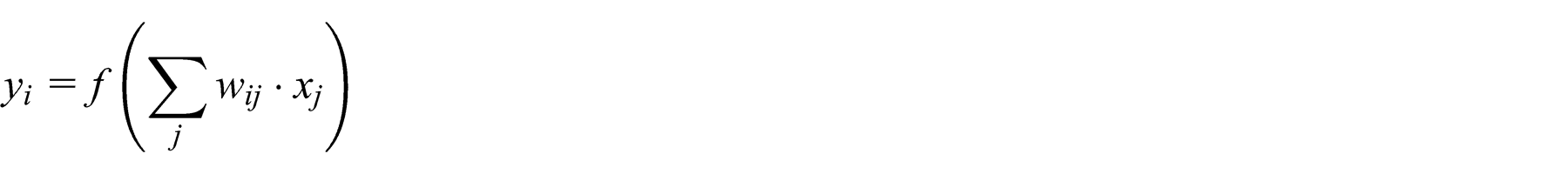
At a computational level, this can be achieved by the presence of multiplicative sub-networks that enable a first (programmer) network to provide input values to a second (interpreter) network through auxiliary input lines. More in detail, the dynamic behavior of an artificial neural network can be defined as an output yi based on the sums of the products between connection weights wij and neuron output signals xj
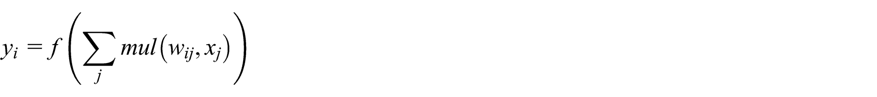
From a mathematical point of view, one can “pull out” the multiplication operation wij ·xj by means of a multiplication (mul) sub-network that can compute the result of the multiplication between the output and the weight, inputs to the mul sub-network
This procedure (called w-substitution in Donnarumma et al. (2012)) is at the basis of the construction of a PNN with a line of auxiliary inputs capable of modulating its behavior “as if” the synaptic efficacies were varied (see Figure 1). As a consequence, a PNN gets the results of receiving two kinds of input lines: auxiliary (or programming) input lines and standard data input lines. The newly introduced programming inputs are meant to be fed with a code, or program, describing the network to be “simulated”.
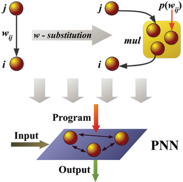
The “pulling out” of the multiplication (on top) performed by means of the w-substitution procedure. Distinct mul networks “break” weights in order to effectively implement a PNN that acts as an interpreter of neural programs.
In principle, a PNN architecture can be implemented using several kinds of recurrent neural networks. Here we introduce an implementation of PNN using Continuous Time Recurrent Neural Networks (CTRNNs), which are generally considered to be biologically plausible networks of neurons and are described by equation (1) (Beer, 1995; Hopfield & Tank, 1986)
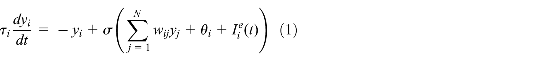
where i ∈ {1, …, N} and N is the total number of the neurons in the network. Thus, for each neuron i:
τi is the membrane time constant;
yi is the mean firing rate;
θi is the threshold (or bias);
σ(x) is the standard logistic activation function, i.e.
wij is the synaptic efficacy (weight) of the connection coming from the neuron j or external sources xj to the neuron i.
The equation (1) has a solution of
Following Donnarumma et al. (2015b, 2012) it is possible to build a PNN, in the CTRNN framework, that is able to simulate (behaving like an interpreter) the behavior of the encoded CTRNN networks on the data coming from the standard input lines when varying the programming input line.
To this aim, the first step is to build a mul network in the CTRNN framework. A mul can be written as
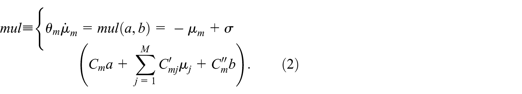
with m ∈ {1, …, M}. Equation (2) describes a network of M neurons receiving two inputs, a and b; the m-th neuron has time constant thetam
, mean firing rate μm
,

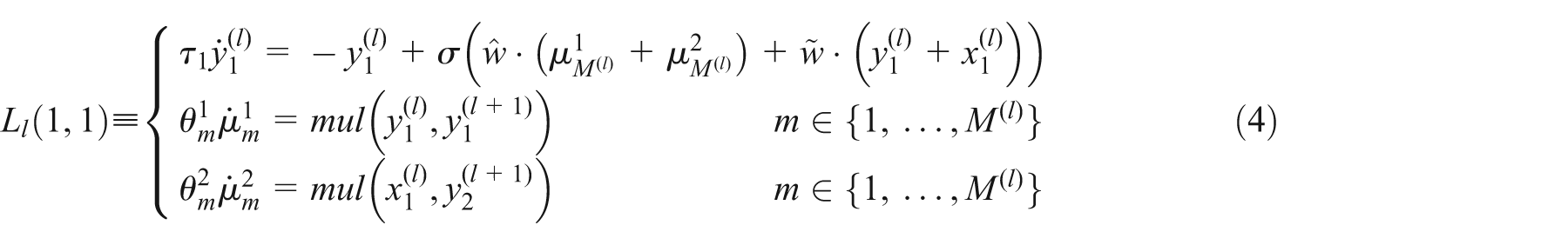
A depiction of the system of equations (4) is given in Figure 2. The Layer is a PNN composed of a slow neuron of activity
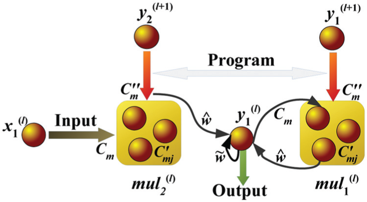
Depiction of a Layer Ll
(1, 1) described in the system of equations (4). The Layer is a PNN composed of one slow neuron
Equation (4) can be straightforwardly generalized to accomplish N (l) slow neurons and Q (l) input sources
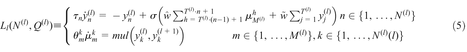
where
we set
the condition on the time constants
The output of a PNN can be redirected as an input of a new PNN, i.e. this computational scheme can easily be iterated at multiple hierarchical layers, with the result that a network playing the role of programmer relative to a lower-level interpreter can also play the role of an interpreter relative to a higher-level programmer, providing a homogeneous hierarchical organizing principle that extends over an indefinite number of layers (see Figure 3).
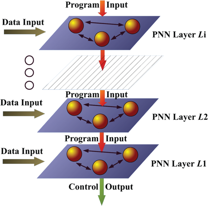
Hierarchical multi-layer architecture of the programmable neural network (PNN) architecture. In the proposed scheme, the upper layers send programs to the lower ones that act, in their turn, as a neural interpreter.
Notice that for an ideal mul, the solution of Ll (N (l), Q (l)) restricted to the slow neurons

when varying the programming inputs

In other words, a PNN system performs a substitution of variables which lets the programming inputs vary the system in the same way the changing of weights does in an “ordinary” CTRNN. When an approximated mul is given, however, it is a difficult task to formally establish an ε bound for large networks (Donnarumma, Murano, & Prevete, 2015a), thus the fine-tuning of the system relies on experimental considerations and can be improved in a way to satisfy Condition (3): (a) by increasing the “speed” of the mul networks tuning the setting of time constants in order to improve the approximation
Finally, we stress that in our modelization, all the connections of the layers are fixed connections and thus, the dynamic behaviors they exhibit are completely due only to the change of their input, i.e. data input
3 Experiments
We present a Hierarchical Programming Neural Network Architecture (HPNNA) built for a robotic scenario. We considered an agent learning eight different tasks corresponding to eight different goals in a T -maze environment (see Figure 6), starting from a fixed start location. The HPNNA is composed of two interpreters of networks (PNNs): a (higher) level L 2 and a (lower) level L 1 (see Figure 4).
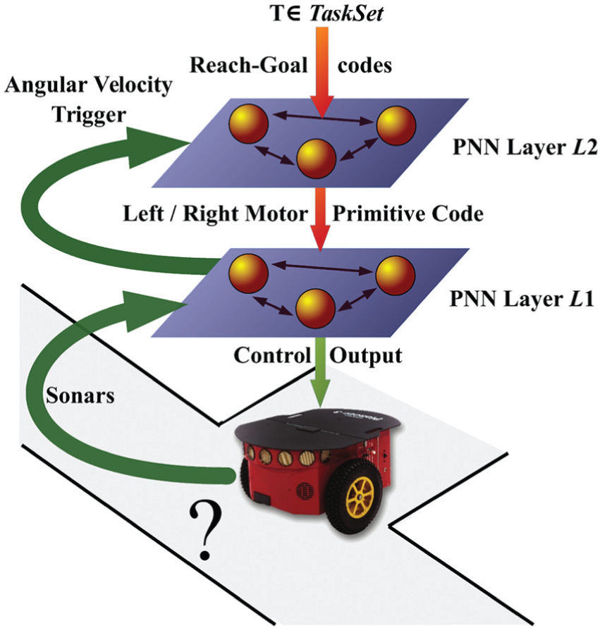
The hierarchical programmable neural network architecture built for the robotic scenario. Two layers of interpreters (PNNs) are present: a (higher) level L 2 and a (lower) level L 1. L 2 receives reach-goal codes on the programming input lines and trigger signals on the data input lines. L 1 receives motor-primitive codes, from L 2, on the program input lines and sensor data on the data input lines and outputs the control signals which govern the robot in the environment.
L 2 receives reach-goal codes on the programming input lines T and trigger inputs on the data input lines from L 1. L 1 receives motor-primitive codes, from L 2, on the programming input lines and sensor data on the data input lines and outputs the control signals that govern the agent in the environment. L 1 can be programmed to implement different motor primitives when its programming input lines are fed with suitable codes. The trigger signal encodes the completion of a motor primitive. L 2 can be programmed to implement different sequences of motor-primitive codes when its programming input lines are fed with suitable codes.
The programming input learning is achieved by a two-step learning strategy which can be described as follows;
In the first step we sought 23 reach-goal codes for the programming input lines of L 2. The learning ensures that when L 2 is fed with one of these codes, the agent is able to perform a sequence of three consecutive motor primitive programs constituting the reach-goal program. The switch between the motor primitive programs occurs when L 2 detects a T-intersection by means of the trigger signal coming from L 1.
In the second step we sought two different lower level programs, Right-Wall Follower (Pr ) and Left-Wall Follower (Pl ), which encode the basic motor primitives of our control architecture. The agent exhibits two different behaviors in the environment according to two different codes Pr and Pl . When L 1 is fed with the programming input Pr or Pl the robot follows the wall to its right or its left, respectively.
In Subsection 3.1 we show the first learning step, preparing a synthetic dataset, in which the stimuli and the programs are simplified in order to study the different learning properties of the proposed architecture versus a non-programmable one. The second step is presented in Subsection 3.2 where the primitives are actually learned in a simulated robotic environment and then the overall architecture is tested in the multiple T-maze simulated robotic scenario.
3.1 Learning motor primitives composition - HPNNA versus NOA
The task of this section is the learning phase of the L 2 PNN module. The aim of the learning is to endow L 2 with the capability of driving the agent in a multiple T-maze environment by sequencing specific motor primitives (see Figure 5).
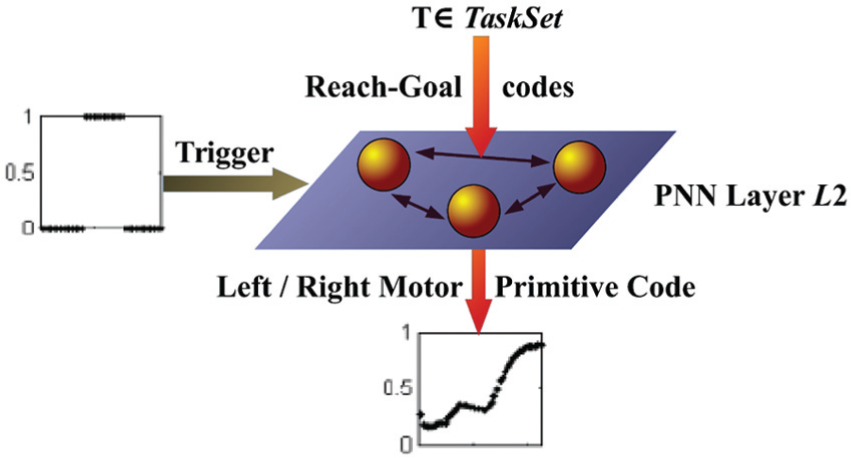
General presentation of sought L 2 module. Its output controls the activation of the proper motor primitive Pl or Pr . It has two inputs, a reach-goal code on which the coded task is presented, and a Trigger input, carrying the information on when the proper primitive should be enacted.
Following from Yamauchi and Beer (1994), we sought a network capable of changing its state when an external trigger is given. Let us suppose we have a network that selects the two programs Pr and Pl by means of the output of one of its neurons. A high value of this neuron selects the program Pr while a low value selects the program Pl .
In order to test how able the proposed architecture is to learn different programs, in this section we prepare a synthetic dataset in order to capture the stylized different tasks in a multiple T-maze code. We compare our HPNNA versus a traditional non-organized architecture (NOA, see below) showing how learning multiple behaviors is computationally more difficult with respect to learning multiple behavior codes. In this experimental scenario we imagined an agent exploring a multiple T-maze (see Figure 6). In the considered mazes each corridor has the same length δ. This δ parameter is an environment variable we varied during the experiments.
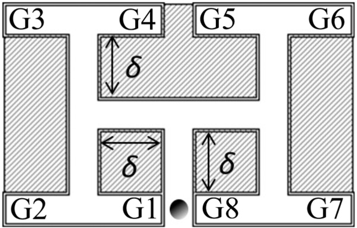
The multiple T-maze scenario used in the experiments. The starting position of the agent is indicated by a gray circle at the bottom of the maze. Each corridor of the maze has the same length δ. G 1, …, G 8 are the eight possible goal positions corresponding to the given task T 1,…,T 8.
Accordingly with our strategy, the control module of HPNNA, sequencing primitives, L 2 has two kinds of input lines:
the data input line is fed with the external trigger;
the programming input line encodes the different sequences that constitute our high level program.
Thus, given the fixed structure interpreter L 2, we learn the structure of a neural network memorizing the input codes to be sent to L 2, testing our HPNNA approach. As a comparison a similar learning is performed on a CTRNN layer that it is not structured as in equation (5) but follows the ordinary CTRNN equation (1); we refer to this module as a non-organized architecture (NOA).
By means of layer L 2, the agent is supposed to control two different low-level primitives:
Left-Wall Follower denoted with Pl , i.e. the behavior “follow the wall on the left”;
Right-Wall Follower denoted with Pr , i.e. the behavior “follow the wall on the right”.
We assume to learn a control module of an agent, with two inputs, a task-input T and a trigger-input ID , plus a motor-output U calling the two primitives, Pl or Pr . The agent is supposed to move inside the maze perceiving it with sensors able to detect walls. When it reaches a T-cross, the trigger-input is activated and the agent consequently moves in order to regain the wall performing respectively a left-turn or a right-turn depending on the input task the agent receives.
Each of the eight tasks T 1, …, T 8 corresponds to the successful reaching of one of the goals G 1, …, G 8 in the maze (see Figure 7). Each task of the agent can be decomposed into a sequence of three low-level primitives [P 1 P 2 P 3] with Pi = Pr or Pl . Each sequence is recalled by the corresponding task-input T sent to L 2, i.e.
A depiction of the eight goal-reach tasks T 1, …, T 8 defined for the experimental scenario. They are composed of a series of three motor primitives and correspond to the reaching of the corresponding goals G 1, …, G 8 in the maze.
Therefore each program corresponds to a high level representation of the possible agent’s behaviors. Ideally, at the end of the learning phase, by selecting a task-input Ti , the agent is asked to assume the behavior that allows it to reach the corresponding goal Gi in the maze. It is important to stress that this program formalization does not point at any specific trajectory, but at a sequencing of low-level primitives.
In this test, the trigger-input ID (t) ∈ {0, 1} is the idealization of a time varying input signal: it is high (ID = 1) when the agent is turning (i.e. the agent is at the end of the corridor) and low (ID = 0) when the agent moves forward along the corridors of the maze. In other words, the trigger tells the controlling unit when the robot turns left or right and, therefore, when it is necessary to select the next primitive from the program sequence “stored” in Ti .
In this first experiment we assume the agent moves at constant velocity vA . Consequently, the duration ΔTlow of the low trigger-input can be considered proportional to the length δ of any of the corridors, while the duration ΔThigh of the high trigger-input is considered proportional to the time spent in the turning at each T-cross and is assumed constant across maze dimensions.
Given these conditions, it is possible to define a parameter λ

which corresponds to the size of a chosen labyrinth, with respect to the trigger inputs to the controlling unit.
We build two different synthetic datasets,
By means of the parameter λ this information is implicitly stored in the trigger-input signal. The corresponding Target output O(t) is consequently created in order to create datasets of input-output couples. The aim of learning is to replicate this target on the network output U(t) at each time step. A number of ten target sequences for programs has been created for each maze. A reference sequence is about 40 time steps t = (1/5) ·τ, where τ is the time constant unit used for the neural network modules. This means that dataset
3.1.1 Learning a control module by differential evolution
We adopt a learning algorithm based on an evolutionary approach, Differential Evolution (DE) Algorithm (De Falco, Della Cioppa, Donnarumma, Maisto, Prevete, & Tarantino, 2008; Price, Storn, & Lampinen, 2005). DE is an evolutionary population based algorithm proved to be very efficient in the continuous domain, fitting the case of learning of parameters of neural networks (De Falco et al., 2008). DE addresses a generic optimization problem with m real parameters by starting with a randomly initialized population consisting of n individuals, each made up of m real values. The population is updated from one generation to the next by means of many different transformation schemes commonly named as strategies (Price et al., 2005). In all of these strategies DE generates new individuals by adding to an individual a number of weighted difference vectors between couples of population individuals.
In this experiment the HPNNA learning is assigned an architecture based on equation (5), which is a fixed structure neural network (no synaptic connections are learned for this module), and an input module, that is a neural network that has to “memorize” the different codes allowing the different task. The aim of the learning is to find the programming inputs able to let HPNNA solve the task. The NOA architecture is a full-connected CTRNN of equation (1), without any particular internal structure. In this case, the aim of the learning is to find suitable CTRNN weights able to let NOA solve the presented task. To keep the comparison fair, we keep a similar number of parameters during the experiments. Thus, for both the compared architectures, DE performs a search for solutions in a parameter space
Experimental parameters for the Primitive Sequencing learning task.
The learning procedure is described in detail in Algorithm 1. There is an outer loop which iterates the procedure for Imax . Each program is evaluated separately with a fitness function which is proportional to the distance between the target output Ok of the corresponding program selected by the task input Tk , from the motor output of the control module Uk (t) = U(Tk (t), ID (t)). Thus the fitness value is computed on the set of sequences relative to the program Tk

Control Module Learning
The function
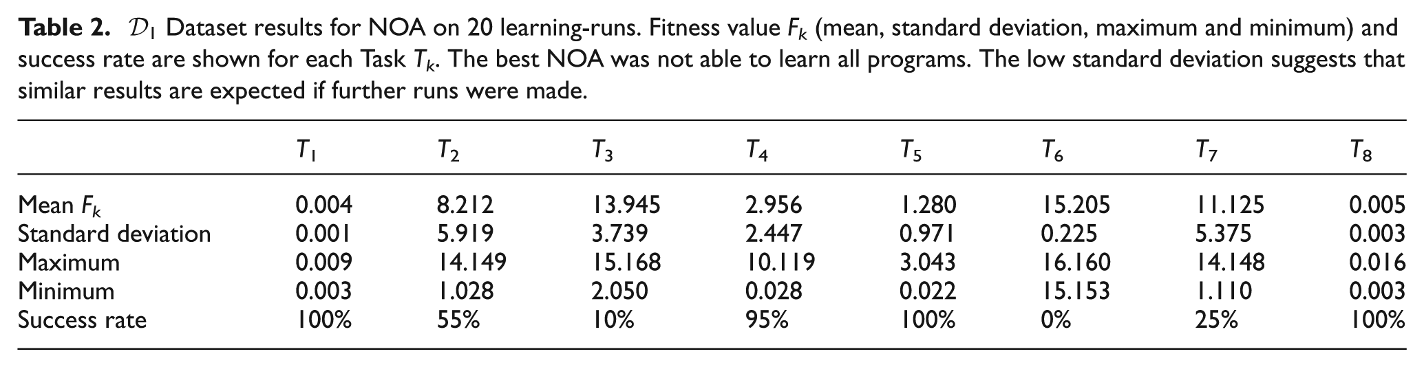
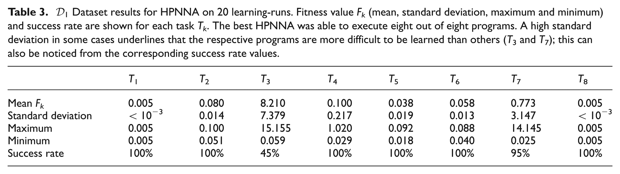
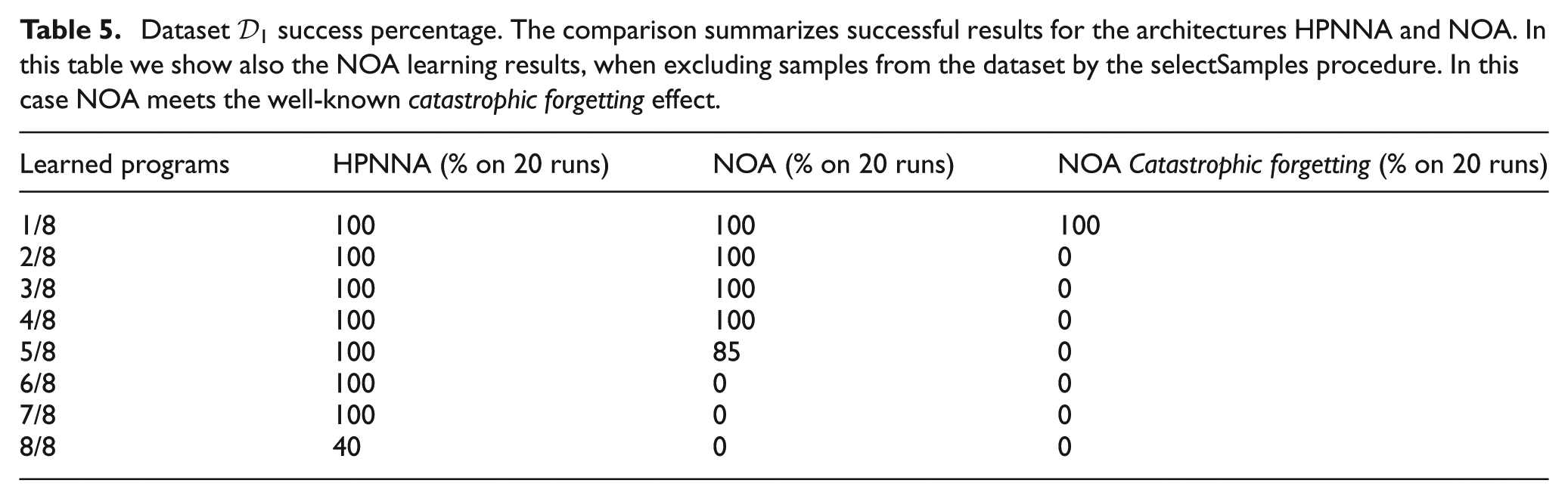
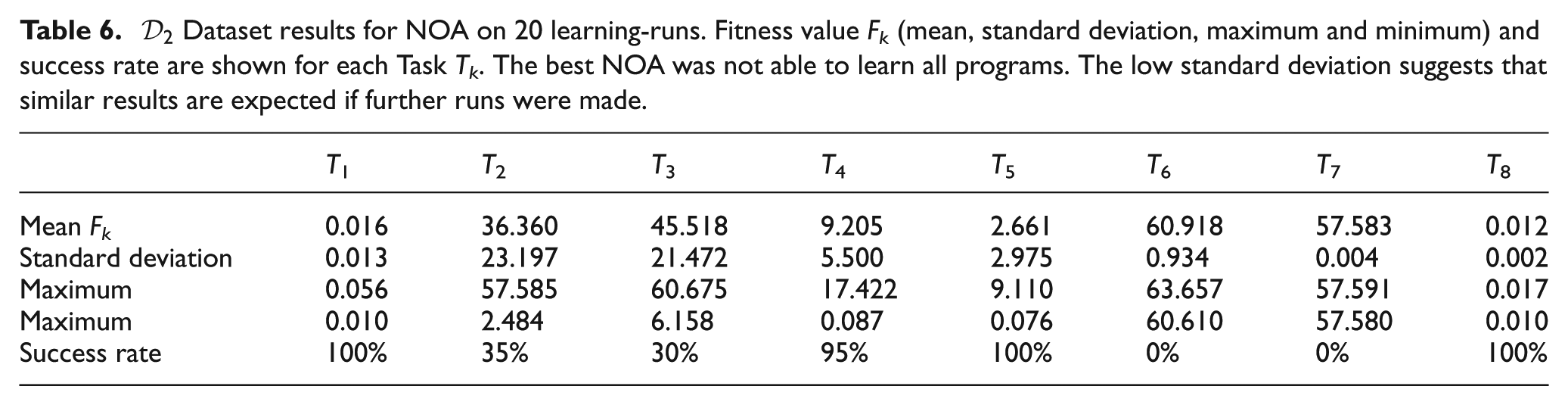
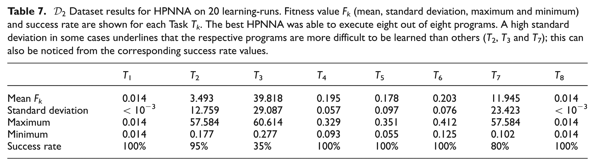
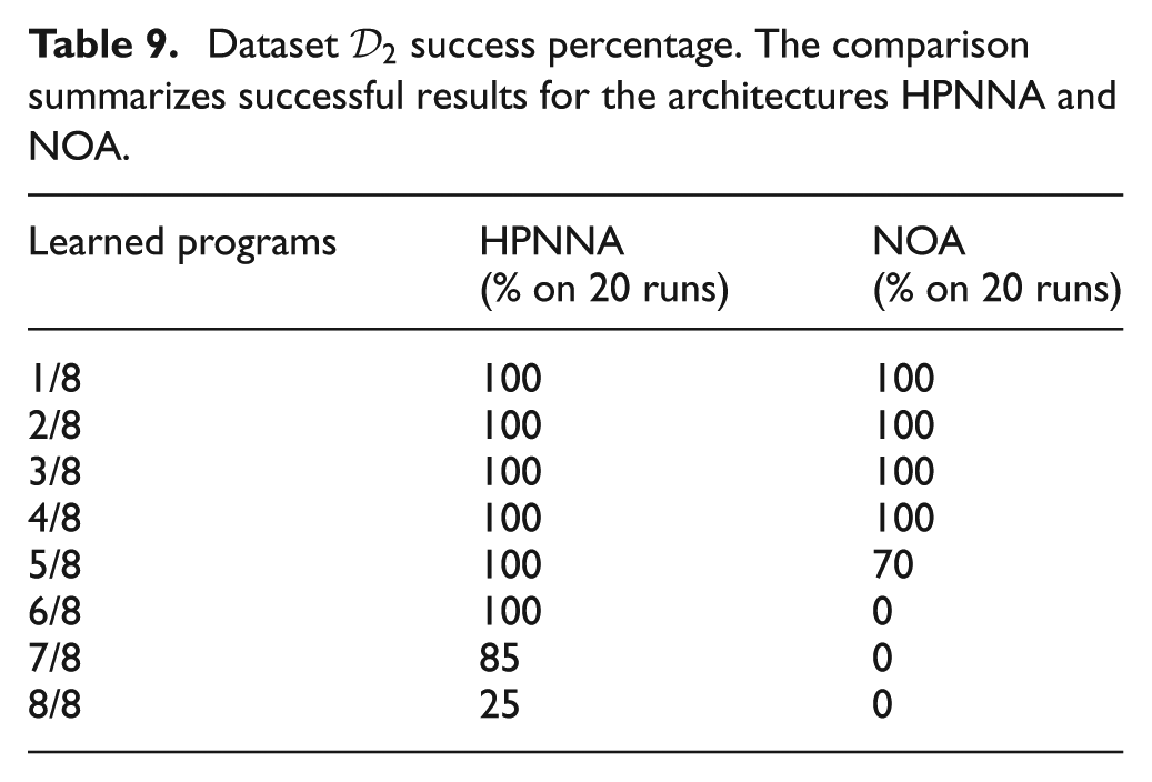
The results of the tests are evaluated by comparing 20 learning-runs for each architecture, HPNNA and NOA. It is possible to see that HPNNA is able to achieve solutions that correctly perform eight out of eight programs. We show:
results in learning
results in learning
testing in maze of δ lengths different from the one seen during the learning phase (see Paragraph 3.1.4).
3.1.2 Learning
dataset – single maze size
Table 2 and Table 3 detail the final fitness value for NOA and HPNNA. For dataset
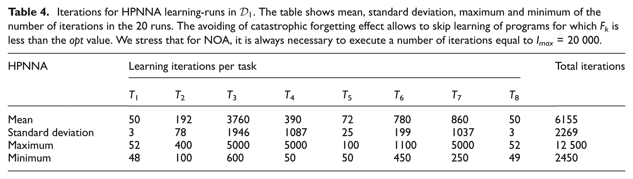
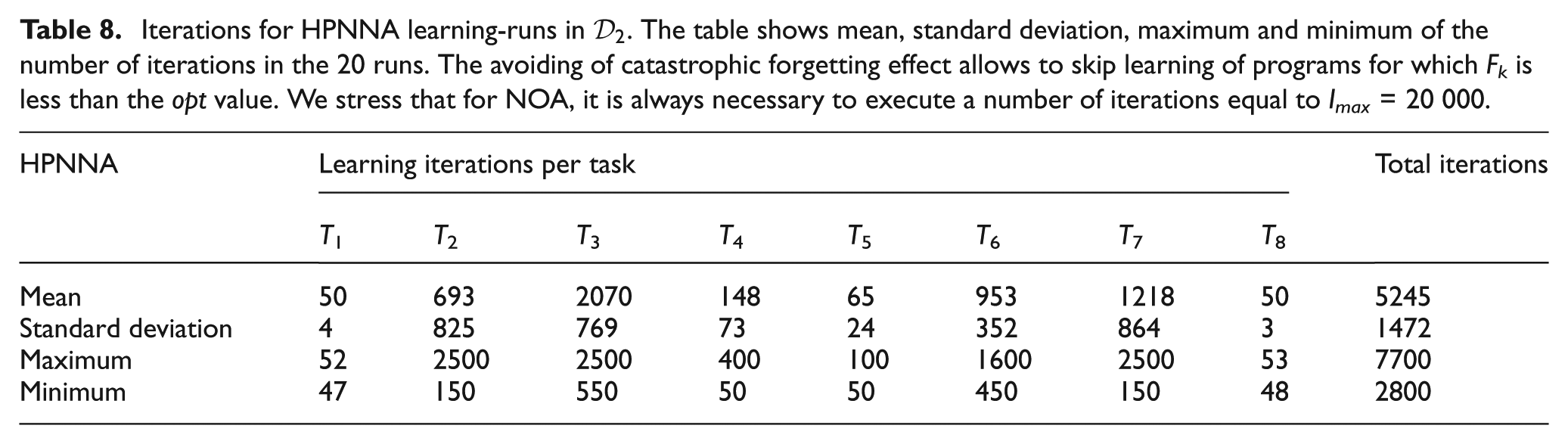
Iterations for HPNNA learning-runs in
Dataset
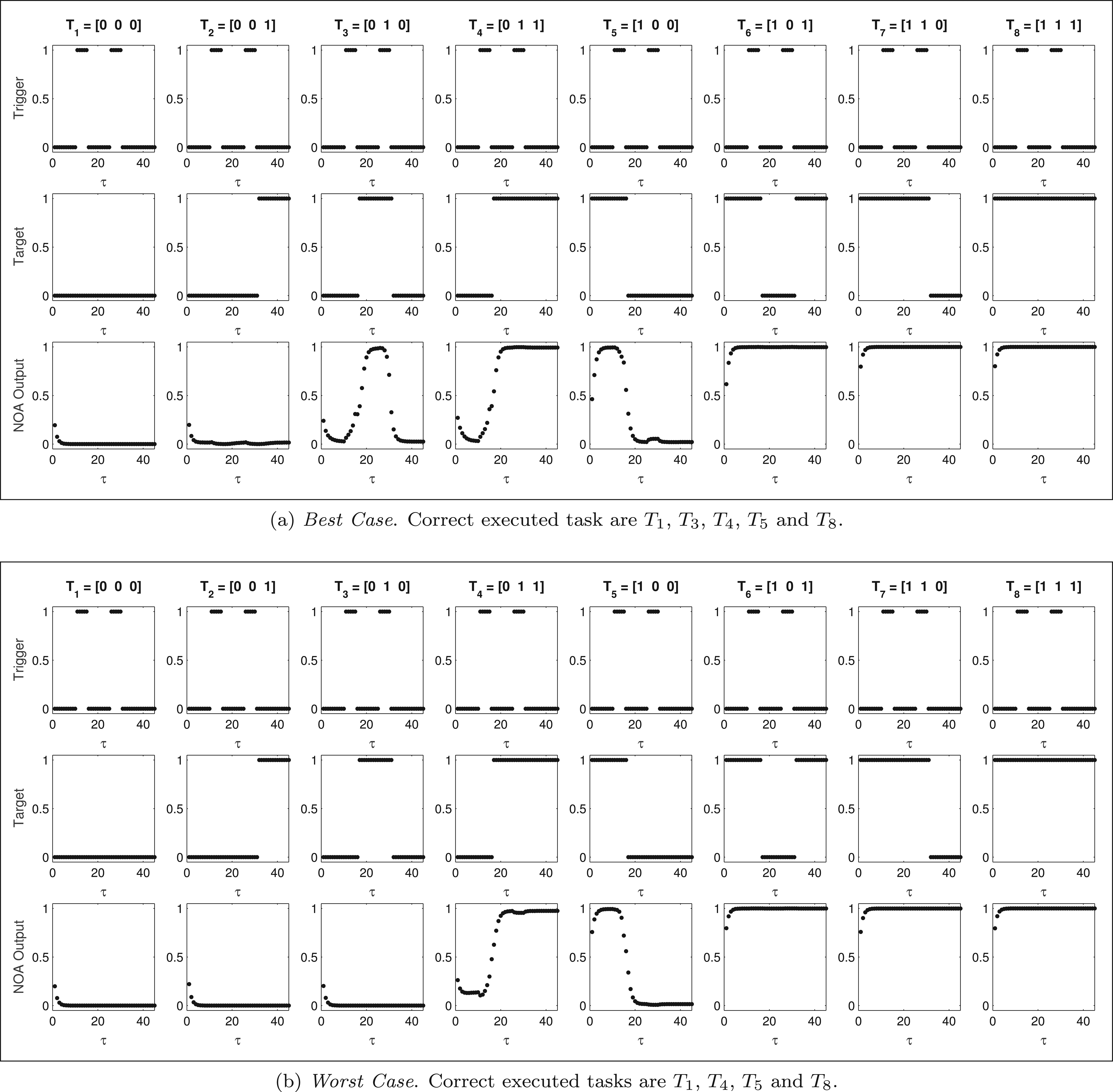
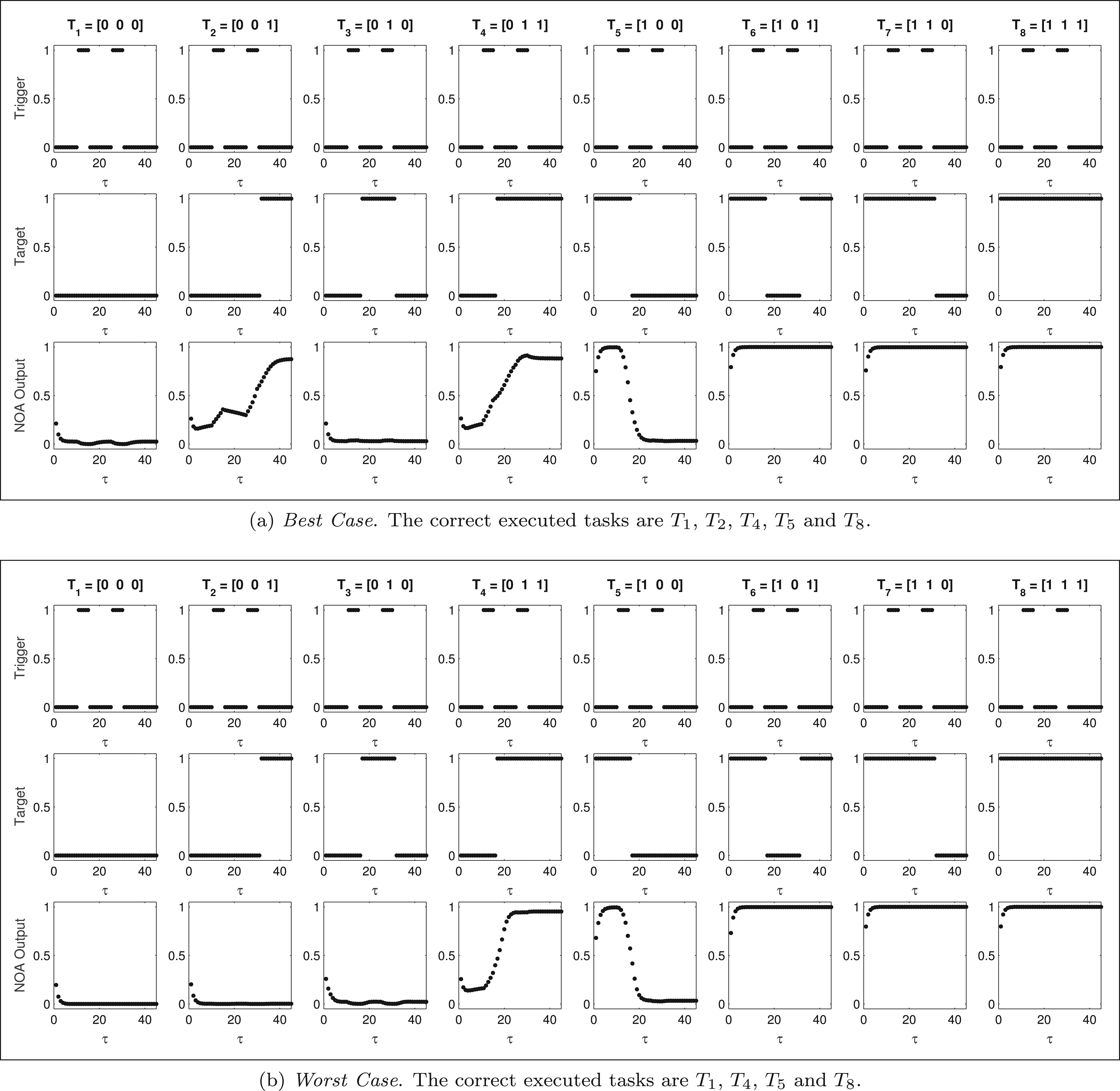
NOA sample outputs for Dataset
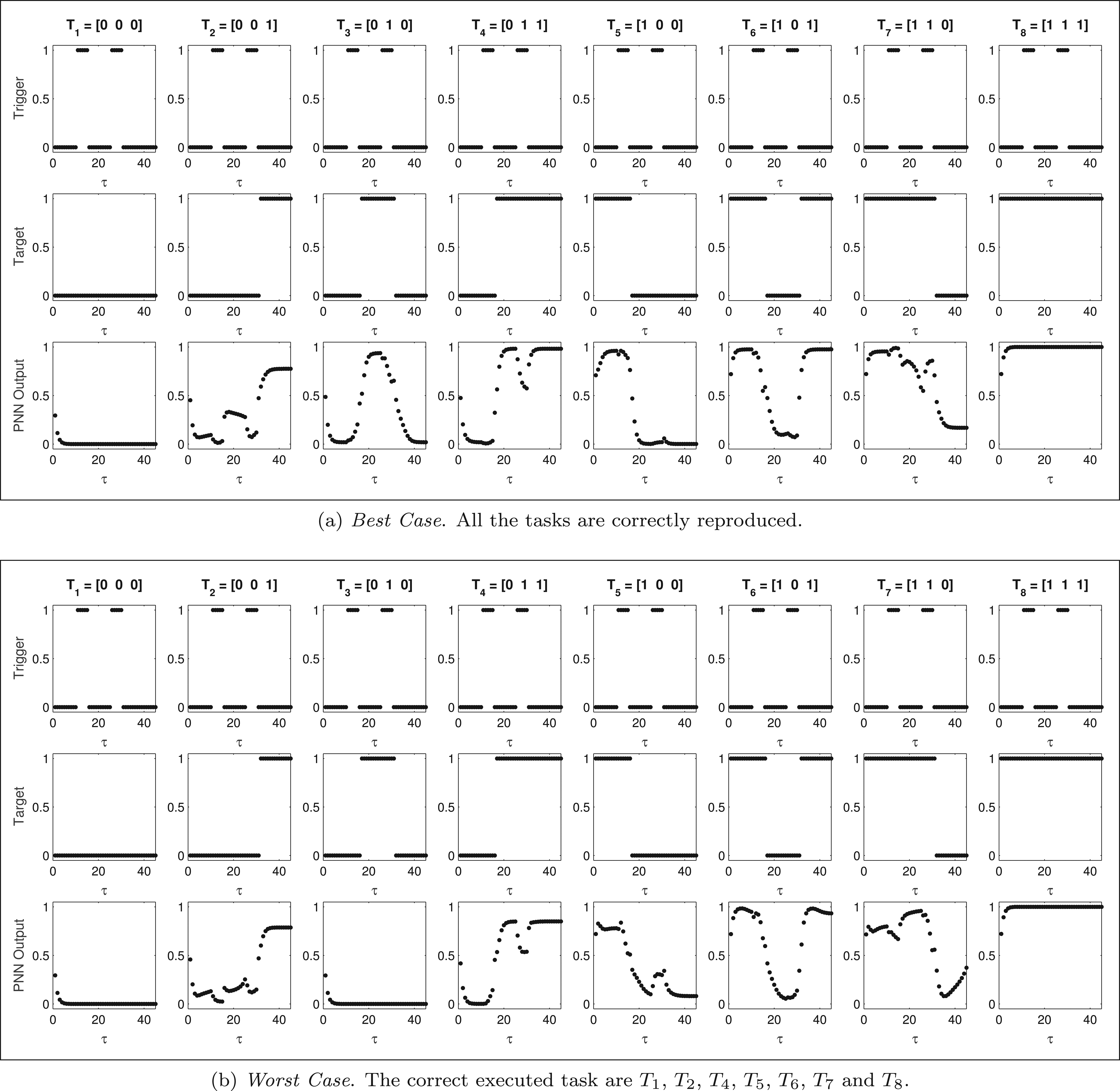
HPNNA sample outputs for Dataset
3.1.3
dataset – three different maze sizes
The dataset
Iterations for HPNNA learning-runs in
Dataset
NOA sample outputs for Dataset
NOA sample outputs for Dataset

NOA sample outputs for Dataset
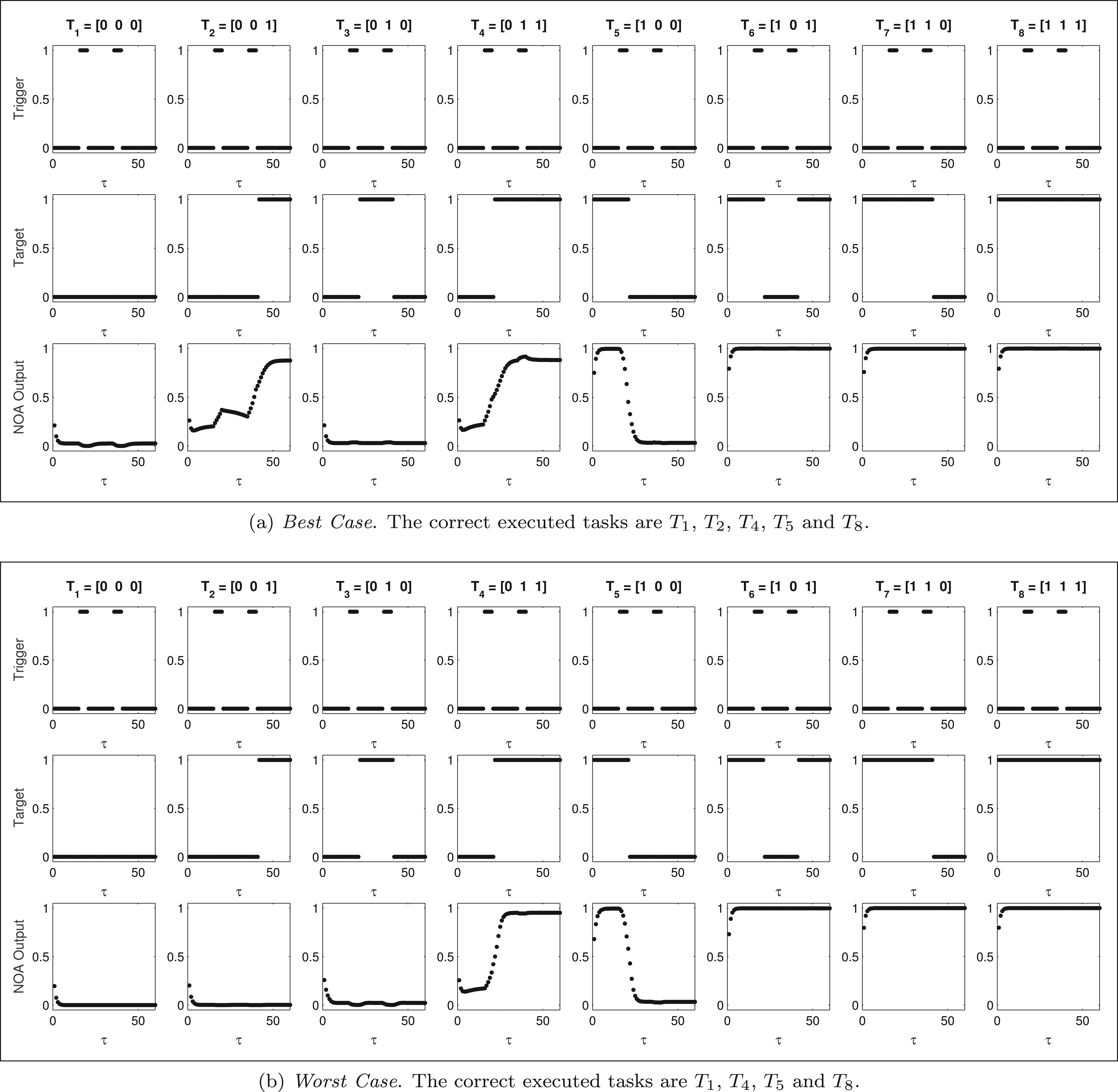
HPNNA sample outputs for Dataset
HPNNA sample outputs for Dataset

HPNNA sample outputs for Dataset
3.1.4 Testing on unknown maze sizes
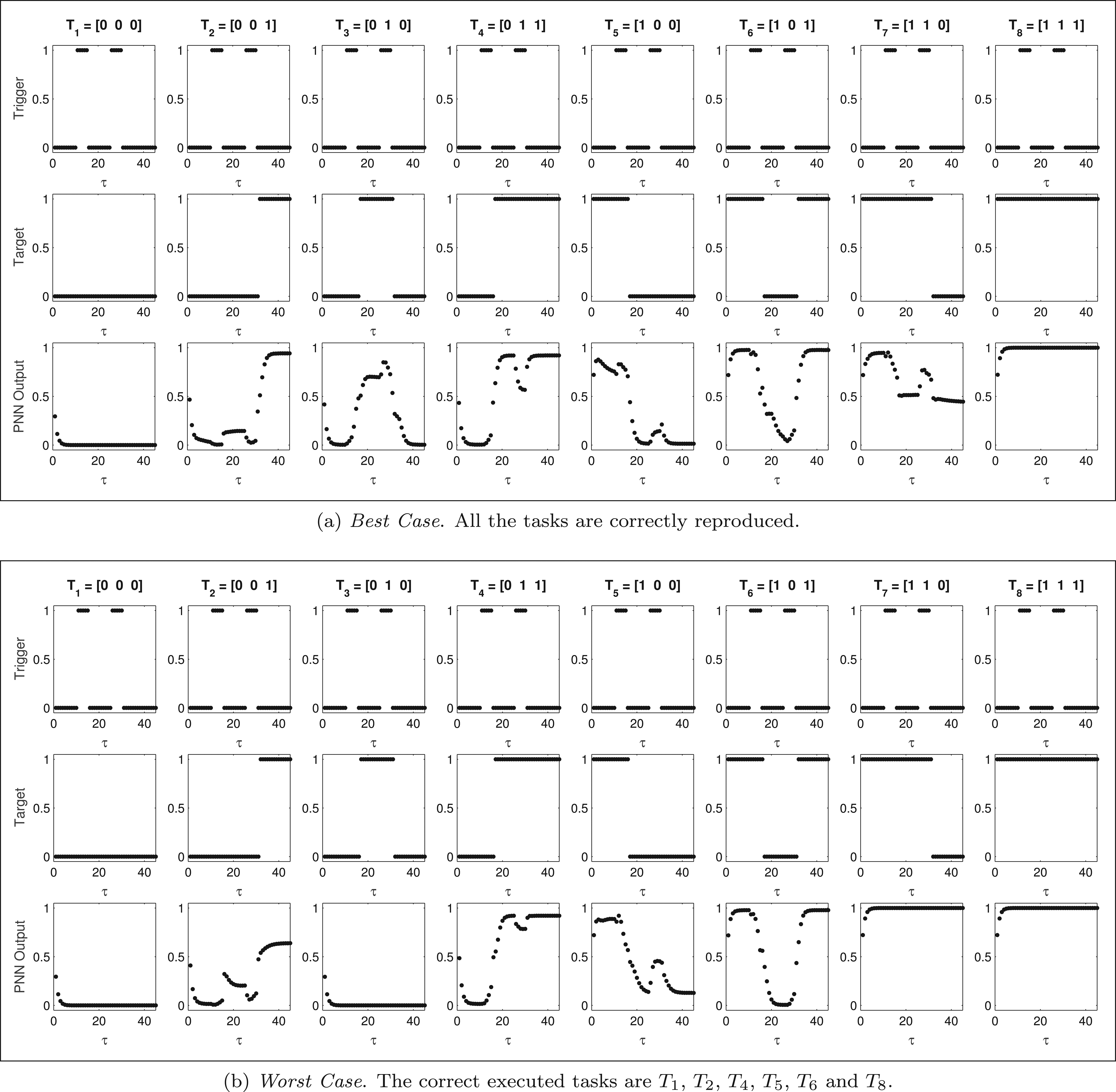
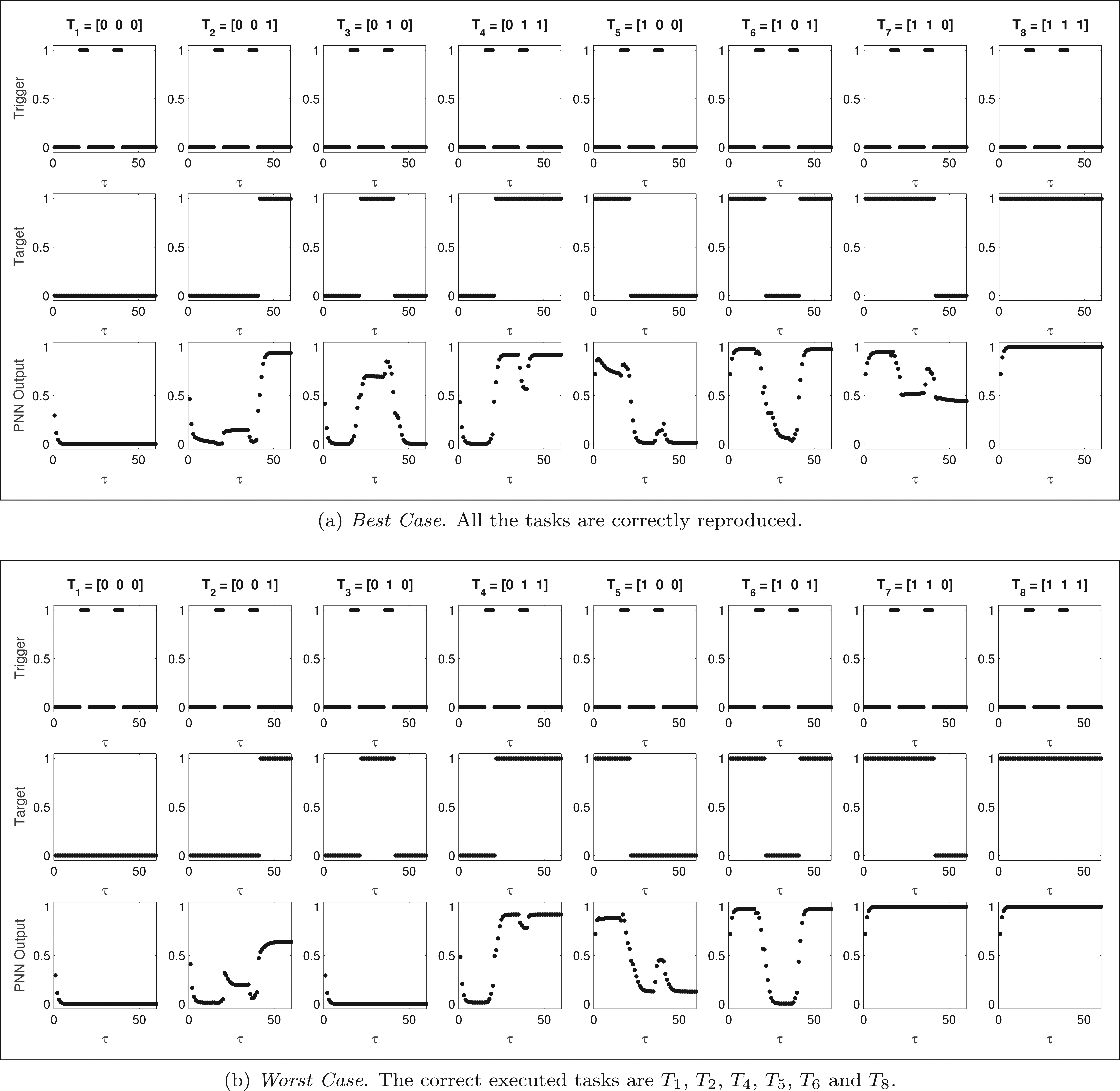
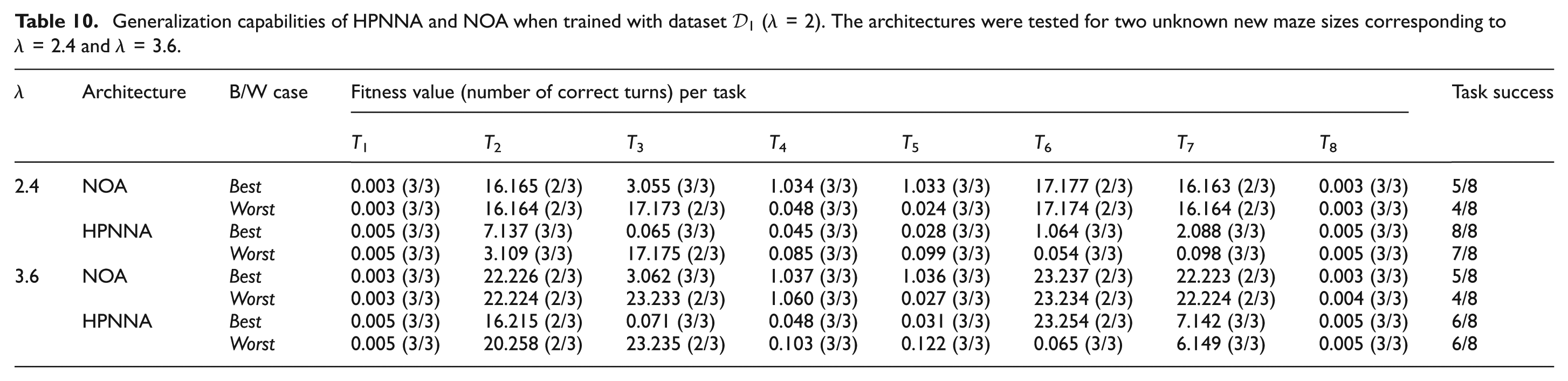
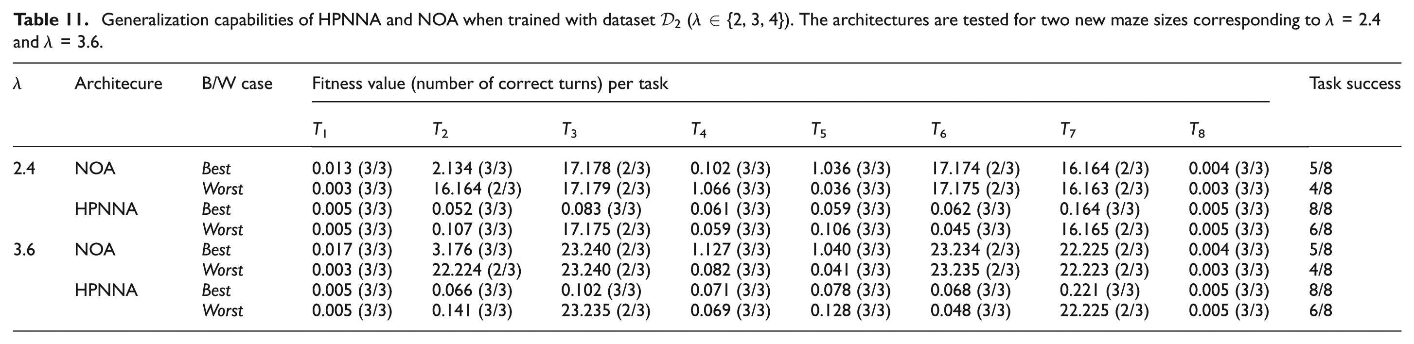
We test all the learned instances of the previous subsections in sequences subsuming mazes of never seen size. This is to verify the generalization capabilities of the architectures. We choose test mazes with λ = 2.4 and λ = 3.6 (see equation (8)). For both the architectures we test best and worst cases learned in datasets
Generalization capabilities of HPNNA and NOA when trained with dataset
Generalization capabilities of HPNNA and NOA when trained with dataset
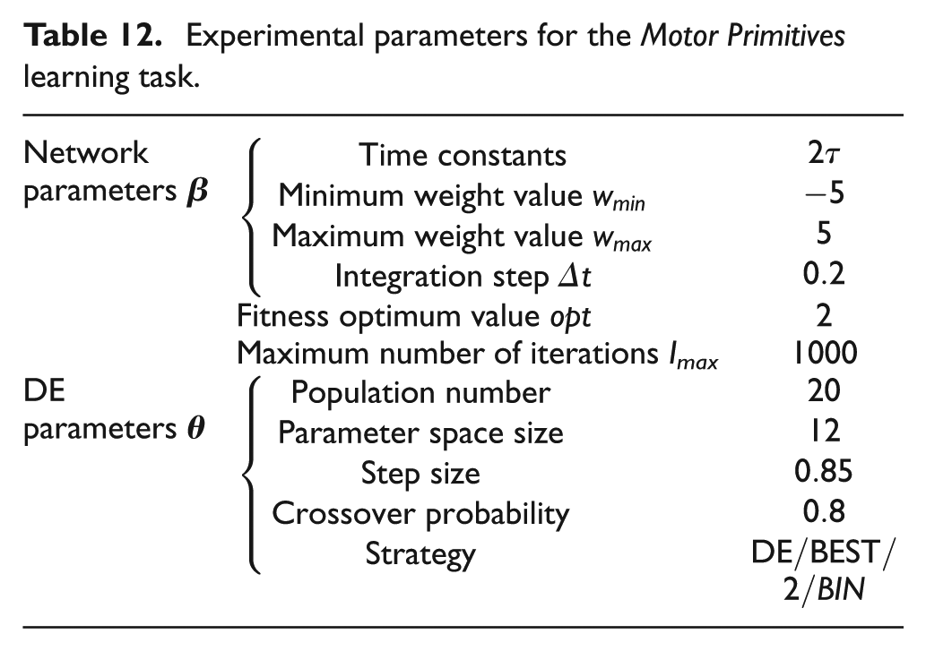
Experimental parameters for the Motor Primitives learning task.
3.2 HPNNA in a simulated robotic environment
In the previous section we made the hypothesis of having ideal motor primitives, in order to build a control module L
2 with suitable inputs to guide the agent towards the desidered goal. In this section we actually implement a lower level interpreter L
1 of motor primitives (see Figure 16) in order to complete the HPNNA architecture and show its performance in a simulated robotic environment. Robot simulations were carried out using the open source software project
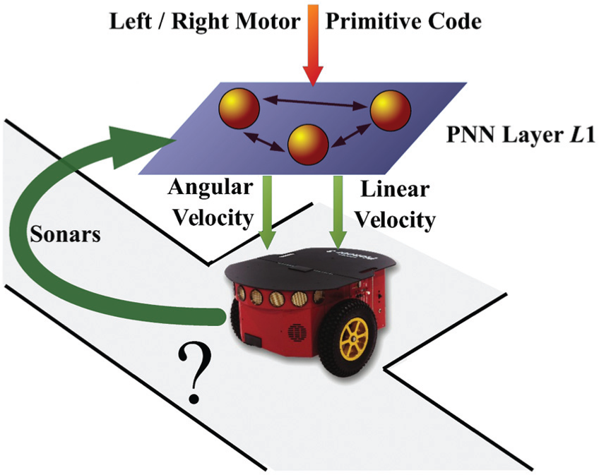
General presentation of the sought L 1 module. Its output controls the Pioneer 3DX angular and linear velocity. It has two inputs, a motor-primitive code and the sonars.
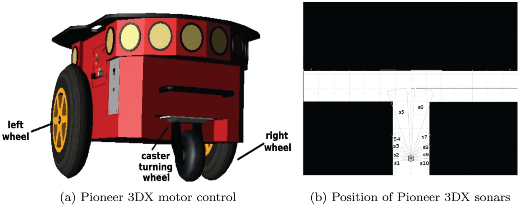
Pioneer 3DX simulation in Player-Stage environment.
Note that L 1 governs the robot by setting its angular and linear velocity corresponding to the output of two neurons belonging to L 1. During this learning phase, the environment is a single T-maze consisting of corridors of fixed length and three times as wide as the robot size.
The L 1 module should realize an interpreter on which two motor-primitive programs are learned: Right-Wall Follower (Pr ) and Left-Wall Follower (Pl ). According to Section 2, this module has two kinds of input lines: a data input line and a programming input line.
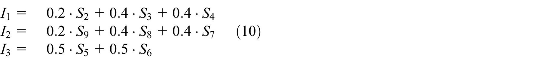
The data input line consists of three inputs {I 1, I 2, I 3} that are the weighted sum of three sonars facing right, the three in which basic motor-primitives are learned facing left and two frontal sonars, respectively, as in the following equations
Thus, two neuron outputs of the L 1 module control the robot. In particular the activation of one neuron is devoted to the control of the linear speed of the robot, while another neuron controls the robot’s angular velocity.
The neurons of the module share the same value of the characteristic time τ, that is of an order of magnitude bigger than the characteristic time of the multiplicative networks θ.
Then, by means of the w-substitution we construct the fixed structure interpreter L 1 made of 39 neurons with two kinds of input lines:
a data input line that consists of the three inputs from the sonars;
a programming input line that consists of inputs that codify the different structures simulated by the interpreter.
Consequently, we evolved a vector of 12 parameters in order to find the suitable programs able to let the network control the robot and perform the correct motor primitives. In our approach, given the fixed structure interpreter L 1, we used Algorithm 1 to learn the suitable motor-primitive codes. This is done by building suitable fitness functions, one for Right-Wall Follower Pr primitive, and a second one for the Left-Wall Follower Pl . Note that, in contrast with other approaches, it is possible to do this because the network structure is fixed and we do not evolve weights. Thus, we can divide the learning into two epochs without erasing previously learned capabilities.
For each epoch we initialized a population of 20 elements controlled by networks with codes randomly chosen in the range [−5, 5]. Each controller obtained is evaluated with a fitness function specific for each program, i.e. FR
and FL
, while performing the task of behaving as a right or as a left follower, respectively. A new population is obtained using the best element of the previous population. In our training we used a crossover coefficient (CR ∈ [0, 1]) of 0.8 and a step-size coefficient (F ∈ [0, 1]) of 0.85, this means that our algorithm builds the next generation preserving the architecture of the best element of the previous generation (the value of the crossover coefficient is low), but even preserving the variance of the previous generation (the value of the step-size coefficient is high). The task used to evaluate the robot is structured as follows. We used a T-maze as the learning environment (see Figure 17b). Each robot is placed at the beginning of each crossroads and it is free to run for about 30 seconds. The final evaluation of the “life” of a robot is the product of the evaluations obtained in each of the distinct simulations. The fitness function that evaluates the robot in every crossroad is made of two components. The first component FM
is derived from the one proposed by Floreano and Mondada (1994) and consists of a reward for straight, fast movements and obstacle avoidance. This component is the same in the left and the right-follower task. The second component changes between the two epochs; in the right-follower training it rewards the robot that turns right at a crossroads (FR
), in the left-follower training it rewards the robot that turns left (FL
). In equation (11)


In FR the average measure of the left sonars over the task period is subtracted from the average measure of the right ones, the opposite happens in FL .
In Figure 18 we show the mean fitness evolution per step of the motor primitives. The interpreter L 1 fed with the best evolved code programs was tested placing the robot in ten different positions in the maze and observing the robot behavior while driving through the crossroads three times. The positions were chosen in such a way that the robot starts its test in the middle of a corridor, oriented with its lateral part parallel to the wall. We tested one code at a time for each execution without dynamically changing the values. In these conditions the interpreter L 1 fed with Pr and Pl was successful in all the trials, showing the appropriate behavior in each of the corridors: L 1 was able to control the robot without crashing and preserving the right motor primitive.
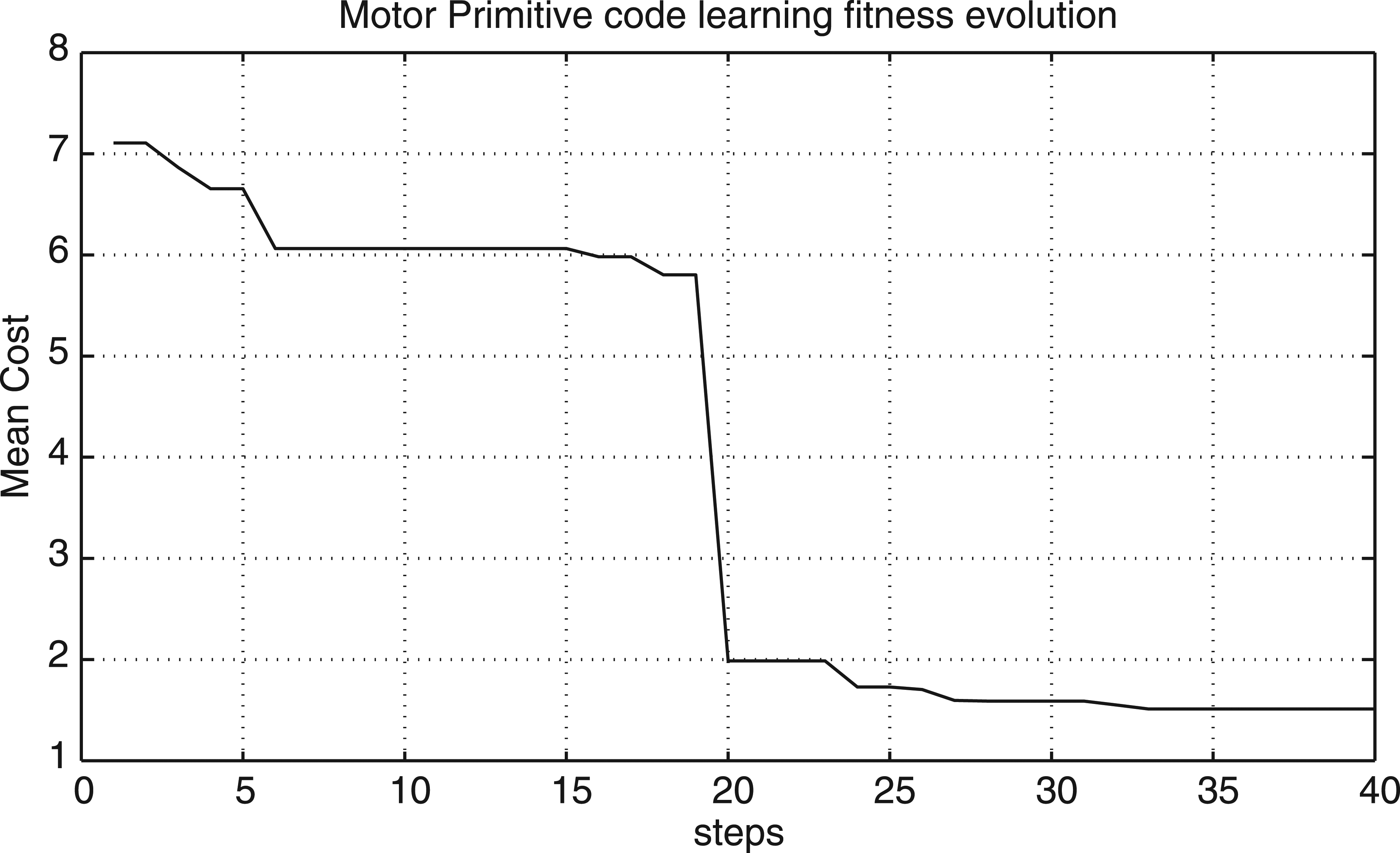
Mean cost evolution per step in Motor-Primitive code learning in the simulated robotic environment.
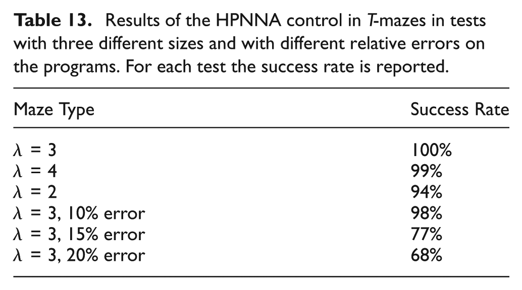
Finally, we show the results of the whole HPNNA control framework in mazes of the kind of Figure 6, for all possible programs learned in the exploring behavior experiments. The trigger signal for the higher level interpreter is for simplicity derived from the output of the angular velocity neuron of the first interpreter (however clever triggering signals from the interpreter could be imagined). We tested it on mazes with different sizes (λ ∈ 2, 3, 4). This is to stress that what we learned is not a particular trajectory in an environment but a high level goal encoded by the program and not influenced by moderate changing in the environment. A test is considered successful if the distance from the goal is under a certain threshold and the robot does not crash. Thus, if the robot reaches a place different from the one “programmed” the test fails. Moreover, we stressed the robustness of the programs learned by applying a relative error ε on each learned parameter p during the execution in the maze environment. These noisy parameter values were drawn from a Gaussian distribution centred in the parameter value p and with a standard deviation of ε = k·w/100 where k ∈ {10, 15, 20}.
Table 13 shows the results. The small decrease in performance for shorter corridor lengths is mainly due to the shorter duration of the trigger on the higher level network. High values of relative error make the probability of failure increase in the maze exploring. However even a relative error of 15% does not erase the behavior of the HPNNA preserving a high success rate.
Results of the HPNNA control in T-mazes in tests with three different sizes and with different relative errors on the programs. For each test the success rate is reported.
4 Conclusions
We have proposed a hierarchical programmable neural network architecture, HPNNA, composed of a hierarchy of modules where each module can be viewed both as an interpreter network capable of running different programs without modifying its synaptic connections and as programmer network capable of controlling the behavior of the lower modules. This implies that the same neuronal substrate can encode multiple motor primitives. Furthermore, the motor primitives can be learned incrementally by increasingly adding more programs to the interpreter network. The learning of primitives in a lower level is transferred to the higher level; new primitives can be added in a fixed lower level by searching for the corresponding programming inputs that the higher level should send. We explored the parameter space resulting from this modelization by means of an evolutionary-based learning approach. The programming inputs of a higher level are fixed with respect to the dynamics of its corresponding lower level, thus learning multiple behavior codes (programs) resulted in being computationally simpler with respect to learning dynamics of multiple behaviors. We successfully tested the performance of the HPNNA architecture in tasks of increasing complexity. Our proposal has implications from both neuroscientific and computational perspectives as we discuss below.
4.1 Neuroscientific perspectives
From a neuroscientific perspective, we present a novel proposal on (hierarchical) action organization and control by the brain, which can be summarized as an interpreter-programmer computational scheme. The interpreter network is able to store multiple action primitives within a common neural substrate. Not only is this encoding scheme parsimonious, avoiding the shortcomings of strong modularity, but it also affords flexible and plausible cognitive control by the programmer network. The programmer network can enforce rule-like behaviors by instantaneously instructing the interpreter network, without the necessity of re-learning. Such fast switches of behavior are the hallmark of cognitive control.
The system learns to represent goals (encoded in the programming input), not trajectories in the environment; this affords the flexible adaptation to changing environmental conditions (e.g. moderate changes of dimensions and sensory cues in a maze). Furthermore, the proposed computational scheme can be iterated to realize hierarchies having increasing levels of complexity (as a network playing the role of programmer relative to a lower-level interpreter can also play the role of an interpreter relative to a higher-level programmer). This provides a novel organizing principle for cortical hierarchies and their role in supporting goal-directed actions.
Overall, the proposed interpreter-programmer scheme is consistent, on the one hand, with the idea of multiple motor primitives in (pre)motor areas (Rizzolatti, Camarda, Fogassi, Gentilucci, Luppino, & Matelli, 1988), and on the other hand with control- and information-theoretic approaches to prefrontal cortex (Koechlin & Summerfield, 2007), and with its role in biasing (instantaneously) behavior (Miller & Cohen, 2001). At the same time, it goes beyond theoretical proposals on executive functions and suggests a plausible neural mechanism (programmability) for exerting cognitive control, which is based on the idea of “reusable” or “recycled” neuronal networks (Anderson, 2010; Dehaene, 2005) (and is therefore alternative to the idea of “gates” and of strongly modular networks). Further studies are of course necessary to evaluate the merits of this proposal, but it has to be noted that its computational parsimony, robustness and scalability (compared to alternative proposals) could offer advantages from an evolutionary viewpoint.
4.2 Computational perspectives
From a computational perspective, this architecture has numerous advantages. Concerning learning, the framework permits incremental learning and the separation of learning phases in different epochs. In fact, it is certainly possible to learn the same behavior in a “classical” way, by learning the weights of a network that at the same time receives the trigger and a program. In that case, one can apply two different strategies: (a) to train a single network able to exhibit all the behaviors; (b) to train one specific network for each behavior so as to obtain eight networks performing the desired behaviors. However, in both cases it is not trivial to accomplish this kind of training. In the first case, because one should be forced to learn all behaviors at the same time, which results in increasing difficulty as soon as the number of behaviors increases. In the second case, the drawback is the necessity of constructing a single network that combines different special purpose networks and switches among their output whenever it is needed. Moreover, in both cases it is difficult to add new behaviors to the learned system. Thus, our architecture suggests a promising neural network approach for these kinds of issues (Umedachi, Ito, & Ishiguro, 2015).
Furthermore, the possibility to steer goal sequences entails flexible behavioral control in the face of uncertain and (moderately) changing environments. Robustness of control is also advantageous to scale up the architecture hierarchically. As moderate errors in program values do not change the overall architecture behavior, programs can be used as outputs of other network modules, realizing hierarchies of control. When a hierarchical organization is built, higher-level modules are necessarily slower than lower-level ones, as they need to guide the realization of sequences of actions (Paine & Tani, 2004).
4.3 Open issues
Finally, the proposed architecture can further be improved in a number of directions. Firstly, in our approach the discovery of new input programs lets the level exhibit novel primitive patterns, without having to relearn already acquired behavior (i.e. incrementally). However, this incremental learning may eventually suffer limitations, for two main reasons;
Each hierarchical level has a fixed level complexity, i.e. can simulate networks of a finite size. If the primitive to be learned has a larger complexity, it cannot be added without increasing the size of “slow” neurons of the level.
Each hierarchical level is affected by an intrinsic “precision error” because of the presence of the mul approximation that crucially relies on the settings of the time constants and on a finite number of neurons M. In other words, an output noise on the mul networks is present that could prevent the learning from adding the wanted novel primitive behavior.
In both cases, the changing of a hierarchical level structure exposes the cost of potentially disrupting all previously learned primitives. A future modeling improvement would be to add a mechanism capable of augmenting the structure without disrupting the existing programs.
Moreover, in our hierarchical scheme implementation, each level receives a “standard” data input that can be an external sensory input (as in our tests with sonars in L 1). In principle, the L 2 data input could rely on some other sensor output, however in our tests we showed that, as a matter of fact, the trigger information on T -intersection detection is already contained in the outputs of L 1. As a general consideration, in our scheme, it is a good idea to include, on the data input line, a feedback input coming from the lower level that could bring information on the timing of the task. However, possibly other (probably lower) levels could bring essential information for the “current level”, so this choice could be somewhat limiting. On the other hand, to include all the levels as a possible input connection would increase computational cost especially for “deep” hierarchies. One line of research would be to add this input choice at a learning level, letting the system decide on the input (coming from the available levels) that maximizes the primitive learning and consequently adapt its connections.
Another open issue is how and where to store the program values in a neural system so that they will be available when needed. This might be met using some reverberant scheme, which in the end will probably require appealing again to synaptic plasticity in ancillary networks. Finally, two lines for future research are assessing the biological plausibility of the proposed model, and advancing more detailed proposals (at the neuronal level) of its mechanisms of learning and recall of the programs.
Footnotes
Acknowledgements
The authors would like to thank Giuseppe Trautteur for the inspiring discussions and comments that greatly contributed to improve the paper.
Funding
The present research is funded by the Human Frontier Science Program (HFSP), award number RGY0088/2014, by the EU’s FP7 under grant agreement no FP7-ICT-270108 (Goal-Leaders). The GEFORCE Titan used for this research was donated by the NVIDIA Corporation.