
Abstract
Achieving efficient and reliable self-organization in groups of autonomous robots is a fundamental challenge in swarm robotics. Even simple states of collective motion, such as group translation or rotation, require nontrivial algorithms, sensors, and actuators to be achieved in real-world scenarios. We study here the capabilities and limitations in controlling experimental robot swarms of a decentralized control algorithm that only requires information on the positions of neighboring agents, and not on their headings. Using swarms of e-Puck robots, we implement this algorithm in experiments and show its ability to converge to self-organized collective translation or rotation, starting from a state with random orientations. Through a simple analytical calculation, we also unveil an essential limitation of the algorithm that produces small persistent oscillations of the aligned state, related to its marginal stability. By comparing predictions and measurements, we compute the experimental noise distributions of the linear and angular robot speeds, showing that they are well described by Gaussian functions. We then implement simulations that model this noise by adding Gaussian random variables with the experimentally measured standard deviations. These simulations are performed for multiple parameter combinations and compared to experiments, showing that they provide good predictions for the expected speed and robustness of the self-organizing dynamics.
1. Introduction
One of the first challenges of swarm robotics is to develop decentralized control algorithms that can lead groups of autonomous robots to self-organize into coherent states of collective motion (Brambilla et al., 2013). A variety of such algorithms have been implemented in simulations, mostly trying to reproduce the collective dynamics observed in biological systems. They have tried to imitate, for example, the dynamics of bacterial colonies (Zhang et al., 2010), ant groups (Mersch et al., 2013), fish schools (Calovi et al., 2014; Gautrais et al., 2008; Tunstrøm et al., 2013), and bird flocks (Bhattacharya & Vicsek, 2010; Cavagna et al., 2013; Toner & Tu, 1995). These bioinspired algorithm could help develop a set of simple core rules for controlling robot swarms and performing other predetermined collective tasks, such as path planning (Sartoretti et al., 2014), spatial formations (Kushleyev et al., 2013; Mathews et al., 2017; Rubenstein et al., 2014; Wang et al., 2014), or collective decision making (Vigelius et al., 2014).
Many of the current collective motion algorithms have been strongly influenced by the Vicsek model (Chaté et al., 2008; Vicsek et al., 1995; Vicsek & Zafeiris, 2012). This is a minimal model that is purely based on alignment interactions, where each agent advances at a fixed speed and tends to align to the mean heading direction of its neighbors. When simulated in a two-dimensional periodic box with noise levels below a critical value, all agents will become approximately aligned and thus move in a common direction. More complex models that use a similar alignment-based mechanism to achieve self-organization have also been introduced. The model in Couzin et al. (2002), for example, considers a three-dimensional system and adds attraction–repulsion interactions to generate group aggregation and avoid collisions between agents. More recently, other models have experiments to address how interactions could depend on other factors, such as agent speed or the choice of interacting neighbors (Bialek et al., 2012; Gautrais et al., 2012; Katz et al., 2011). Despite the differences between these models, they all strongly rely on explicit, Vicsek-like aligning interactions to self-organize into collective motion.
In the context of swarm robotics, a strong reliance on alignment interactions can have several disadvantages. For example, components that detect relative orientations are less common than those measuring relative positions. In addition, each robot will typically have to obtain information not only on the headings of other agents (to implement the alignment-based algorithm) but also on their relative positions (in order to avoid collisions and group dispersion). This implies that all robots must have the necessary hardware to detect both quantities, which increases their cost and complexity. Furthermore, although aligning interactions are effective in achieving self-organized collective translational motion, they typically cannot produce other states of coherent collective motion, such as group rotation 1 (Gautrais et al., 2012). It would therefore be beneficial to implement in robot swarms control algorithms that can achieve collective motion without requiring aligning interactions, that is, without requiring the exchange of orientation information between agents. One such algorithm 2 is the Active-Elastic (AE) model, which was recently proposed theoretically in Ferrante et al. (2013a, 2013b) and first tested experimentally in Ferrante et al. (2012).
In this work, we implement the AE model as a position-based decentralized motion control algorithm for a collective robotics experiment, exploring its advantages and disadvantages in a real-world setting. We show that a system of up to seven robots initially in a nonaligned state can robustly self-organize to a common heading direction and achieve collective motion, even in an experimental setup with significant sources of noise and long processing time-delays. Despite this success in achieving collective motion, we also observe that the AE algorithm is intrinsically prone to small-scale oscillations, which can eventually lead to instabilities. We will identify the origin of these oscillations with a simple analytical calculation that considers only two agents. We then characterize the experimental noise and processing times introduced by real-world limitations, showing that we can closely reproduce the robot dynamics when these are added to our numerical simulations. We thus demonstrate that it is possible to predict the optimal experimental parameter combinations leading to self-organization by simulating the observed noise. Finally, we show that a small variation of the AE algorithm can achieve instead self-organization into collective rotation.
The article is organized as follows. In Section 2, we describe the AE algorithm in its dimensional and nondimensional forms, its self-organizing mechanism, and the order parameters used to monitor its collective states. Section 3 presents our experimental setup and the tests we performed for its validation. In Section 4, we describe the typical self-organizing dynamics observed in our robotic system and characterize its stability and experimental noise. We then compare in Section 5 the typical collective dynamics in our experiments and simulations for different regions of the parameter space. In Section 6, we introduce a variation of the AE algorithm that leads to collective rotation in our experiments. Finally, Section 7 discusses the capabilities and limitations of the AE model for controlling robot swarms, in light of our experimental and numerical results, and presents our conclusions.
2. Position-based control algorithm
In this section, we describe the AE control algorithm and order parameters used in our swarm robotics experiments.
2.1. The AE model
We implemented a decentralized swarm robotics control algorithm based on the AE model introduced in Ferrante et al. (2013a, 2013b). This minimal model was shown to produce self-organized collective motion, even in the presence of noise, when starting from a group of agents with random initial headings. It only requires the exchange of positional information between agents, without requiring any explicit alignment interaction or the exchange of orientation or velocity information.
We used as the control algorithm a noiseless AE model and defined all the interaction forces between agents as having the same strength k0 and equilibrium distance l0. With these simplifications, the AE model is defined as follows
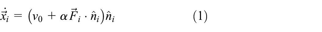

with
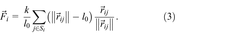
Here,
Equations (1) and (2) determine the forward/backward speed and the angular velocity of each agent, respectively. The system is overdamped: each agent moves faster or slower than its preferred speed
We confirmed in preliminary analyses that AE models with attraction–repulsion potentials that allow changes of interacting neighbors produce similar self-organizing dynamics as the fixed interaction models studied here, but introducing additional complications. If the interaction range is too short, connectivity is broken and the swarm can disband; if it is too long, interactions with second neighbors can produce excessive aggregation. Further studies that go beyond the scope of this article should therefore be carried out to determine the proper nonfixed interaction rules for each scenario. For simplicity and robustness, we will thus only consider here fixed interaction networks.
2.2. Nondimensional form
In order to reduce the dimensionality of the parameter space, we write the nondimensional form of equations (1), (2), and (3) in terms of the system’s natural length and time units, L = l0 and T = l0/v0, respectively. We thus obtain
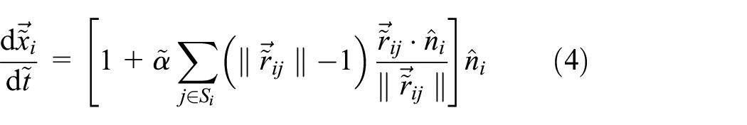
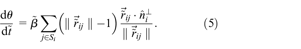
Here, the variables with tilde are nondimensional (expressed in units of L and T) and we have defined the nondimensional effective coupling constants
2.3. Self-organizing mechanism
Given that the AE model has no explicit local alignment interactions that could directly lead to heading consensus, a more subtle mechanism for its self-organization was unveiled in Ferrante et al. (2013a, 2013b). This mechanism is based on a rearrangement of individual headings that favors the injection of self-propulsion energy into lower “elastic” modes of the collective structure formed by all interacting agents. As in standard damped elastic systems, higher energy modes tend to decay faster than lower ones, since they are harder to excite. In this active case, however, each agent is continuously injecting energy through its self-propulsion, so all modes cannot be fully dampened. Instead, through the coupling in equation (2), higher elastic modes decay by steering agents away from them. Self-propulsion thus feeds more energy into lower modes, which have larger regions of coherent motion, eventually achieving self-organization into collective motion at the scale of the whole system. A more detailed explanation of this mechanism was given in Ferrante et al. (2013a, 2013b). In the remainder of this article, we will explore the capabilities and limitations of this mechanism when applied to real robotic systems.
It is important to point out that the scalability of the AE algorithm, for achieving collective motion in systems with a large number of agents, has already been demonstrated numerically in Ferrante et al. (2013a, 2013b). In these papers, simulations with over 3000 agents are shown to self-organize into collective motion. The approaches presented here could therefore, in principle, be applied to larger robotic systems, although further research is needed to show that the real-world conditions explored in this article are also scalable.
2.4. Order parameters
We define here two order parameters that will help us monitor the degree of translational and rotational order in the system, as in Couzin et al. (2002).
First, we consider a quantity that can monitor to what extent robots are aligned and moving in a common direction. The polarization order parameter is thus defined as
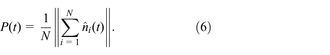
where
Here,

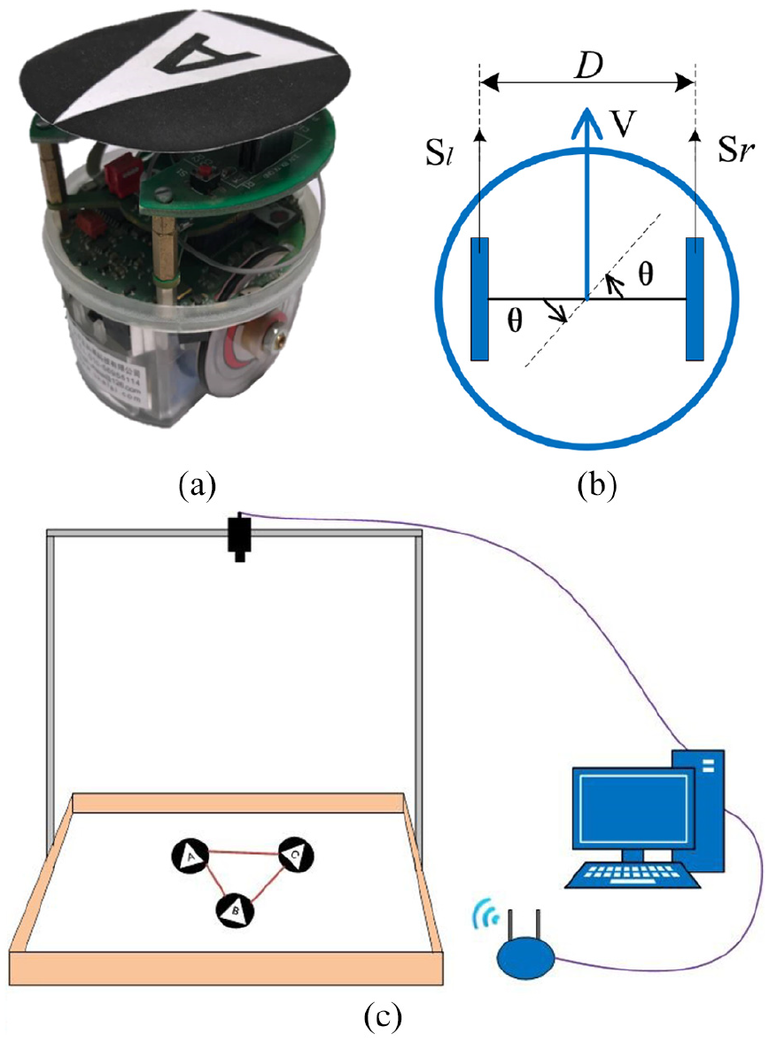
where
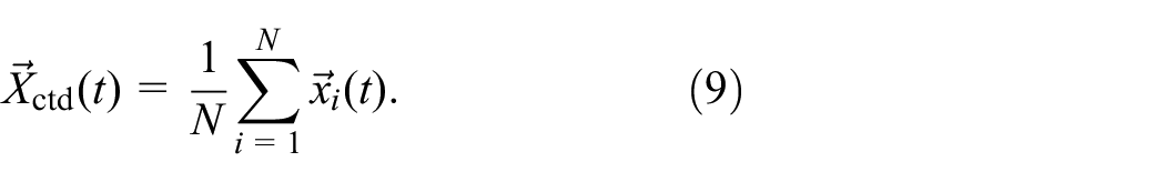
Note that, with these definitions, the values of P(t) and M(t) will both range between 0 and 1. A case with P(t) = 1 and M(t) = 0 corresponds to perfect parallel group translation and a case with P(t) = 0 and M(t) = 1, to perfect rotation.
3. Experimental setup and validation
We describe in this section the details of our experimental setup and three tests that we performed to validate it.
3.1. Agents, arena, and time-step
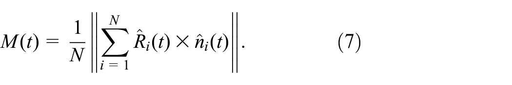
Our experimental setup is presented in Figure 1. We chose the e-Puck robots as our agents (Mondada et al., 2009) because these small differential wheeled robots can be easily manipulated and programmed. They also display the smooth forward, backward, and turning motion required by our algorithm. On top of each e-Puck, we added a Wi-Fi communication module (Hlk-wifi-m04), connected to the processor through its serial port. We can then link a router or a wireless exchange board to all Wi-Fi modules to achieve one-to-all broadcast communication. This allows each robot to receive the relative positions of its neighbors, as well as its own heading, through wireless information from an external computer outside of the arena. Each robot then computes the control algorithm on its onboard processor and moves accordingly. Note that these relative positions and heading could have been, in principle, measured onboard. The only reason for obtaining them off-board in our experiments is that e-Pucks have no onboard compass and very imprecise range and bearing sensors. Our setup thus implements a control algorithm that could be fully decentralized and autonomous (with all sensors and computations onboard) for robots with better sensing capabilities.
Robots and arena setup used in our swarm robotics control experiments. Groups of e-Puck robots, detailed in Panels (a) and (b), are placed on the arena sketched in (c). Each agent receives the position of its neighbors and its own orientation from an external computer, using this information to compute and execute the control algorithm on board: (a) View of a modified e-Puck robot used in our experiments. (b) Diagram of the e-Puck robot structure, viewed from above. (c) Arena and position acquisition system. The overhead camera and the computer detect agent positions, relaying them to the robots via Wi-Fi.
The details of the external sensing system are as follows. We placed a tag on top of each robot with a triangle pointing in its heading direction and a letter (see Figure 1(a)). These visual cues were used to determine the position, orientation, and identity of each robot. We set up a high resolution camera (1928 × 1448 pixels, FLIR Systems, Point Gray Research, model GS3-U3-41C6C) over the arena, pointing down, and linked it to an external computer (see Figure 1(c)). The camera was set at an approximate height of 1.5 m, in order to cover an area of approximately 1 × 1.5 m of the arena (which had a total size of 2 × 2 m), within which the robots were placed and all the experimental dynamics were set to occur. Using this setup, snapshots were taken throughout each experimental run and analyzed by an image processing software. The positions and orientations of all robots were then immediately broadcasted, with each robot receiving through its Wi-Fi module only its own orientation and the relative positions of its neighbors. At every update, the onboard control algorithm thus generated new
Despite requiring additional hardware and a special arena, the external sensing system in our experiments is ideally suited for testing the capabilities and limitations of the AE model. Indeed, since the tracking algorithm and information broadcasting take some time and are simultaneous, they force the
3.2. Validation in a two-robot system
We validated our experimental setup by testing three simple cases of the two-robot dynamics for which we know the theoretical results. In all these tests, we set the equilibrium distance between robots to
Our first test consisted in placing the two robots side-by-side, heading in the same direction, and at the equilibrium distance
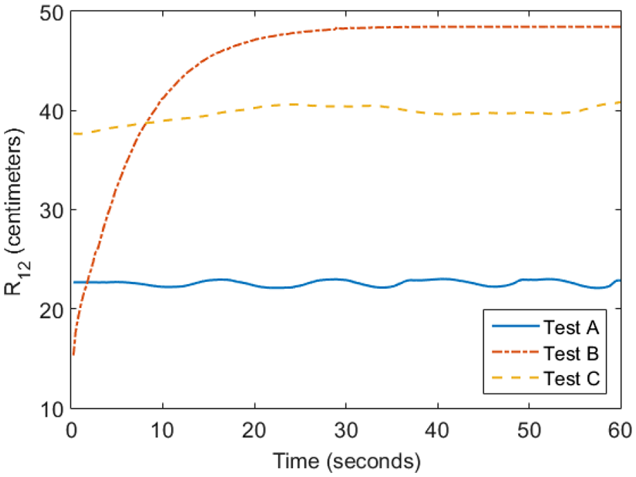
Relative distances, as a function of time, between the two robots used in three simple tests performed to validate our experimental setup (see Section 3.2).
The second test was to place the robots back to back, pointing in opposite directions. In this test, the robots will move away from each other until they reach an equilibrium distance
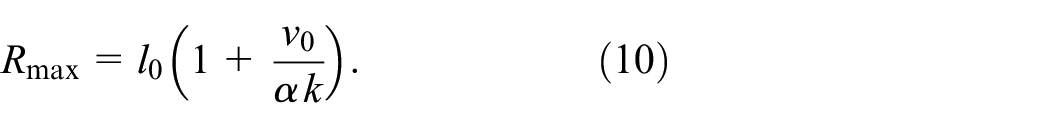
The result of this experiment is presented as curve B in Figure 2 (see also Video SV2 in the Supplementary Material). Given that
In our third and final test, we placed the robots side-by-side, pointing in parallel but opposite directions. We set them at a distance
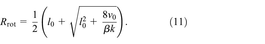
Since we used
The three tests detailed above confirmed that our control algorithm works as expected in simple two-robot scenarios. They also displayed evidence of various sources of experimental noise that can lead to small differences with respect to our theoretical results. We point out, however, that these tests are not a systematic analysis of the precision or reliability of the two-robot system. They only describe our verification method for showing that our setup can match the expected theoretical dynamics. We found that our two-robot trials were always successful when there were no failures in the robots, tracking, or Wi-Fi system (such as mechanical, position detection, or communication issues). They therefore allowed us to debug our experimental setup. In scenarios where the focus is on the performance of a specific system for engineering applications, a systematic study of the two-robot system could provide critical information that can be extrapolated to larger robot swarms.
4. Translational collective motion
In this section, we study the self-organizing dynamics that leads to collective translational motion in our experimental system. We begin by examining the typical dynamics of a group of seven robots in a hexagonal formation and with initial random headings. We then focus on the oscillations in the heading direction that spontaneously appear after the collective translation state is reached. These result in sinusoidal trajectories that are only partially aligned. Finally, we end the section by characterizing in detail the experimental noise measured in our system.
4.1. Typical self-organizing robot dynamics
Figure 3 displays snapshots of the typical self-organizing dynamics observed in our experiments (see also Video SV4 in the Supplementary Material). We overlaid here blue lines on all panels to show which pairs of robots are interacting. We also added large green arrows to Panels (b) and (d) to indicate the group’s heading direction. In addition to these snapshots, Figure 4 plots the corresponding values of the polarization and rotational order parameters, as defined in equations (6) and (7), for the same experiment.
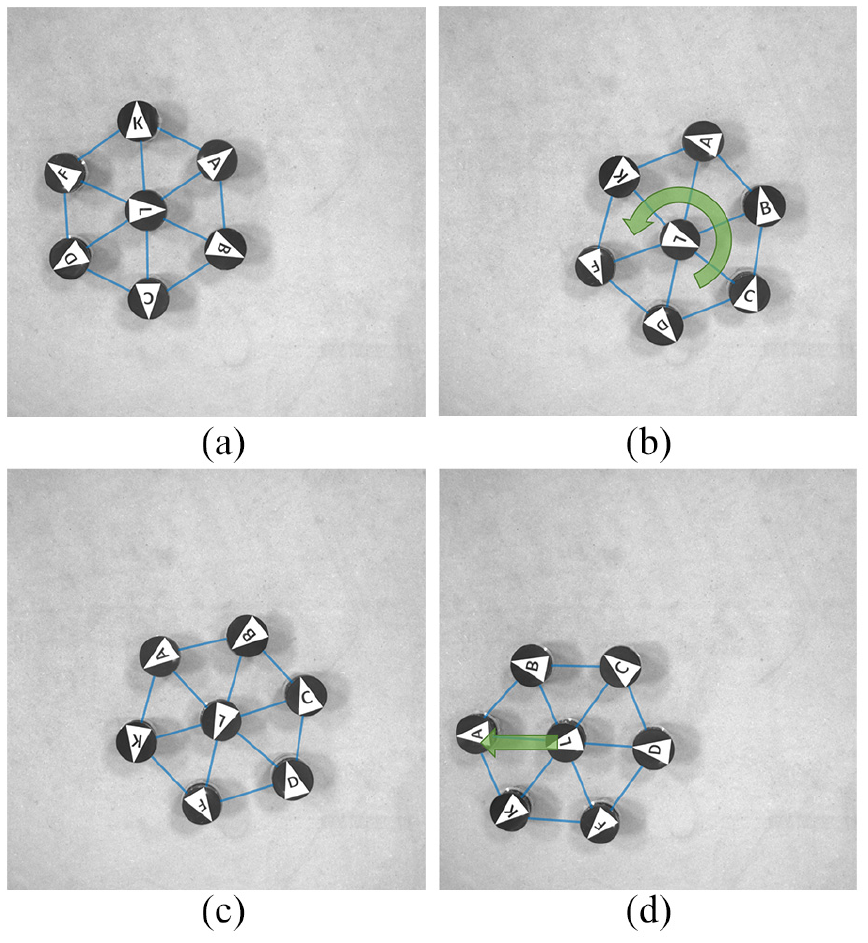
Snapshots of a robot swarm experiment that implements the position-based decentralized control algorithm specified in equations (1)—(3). We observe its typical self-organizing dynamics toward translating collective motion (see video SV4 in the Supplementary Material). The overlaid blue lines indicate which robots are interacting. (a) Standard initial condition used in our experiments and simulations (t = 0 s); robots are placed in a perfect hexagonal configuration with all but the central agent pointing radially outwards. (b) Transient rotating state (t = 108 s); as the system self-organizes, it sometimes first visits a metastable rotational state, as displayed in this panel. (c) Transition to translating state (t = 155 s); the group eventually leaves the rotational state, converging towards translational motion. (d) Final self-organized aligned state (t = 216 s); the system achieves translational collective motion and will move together until it reaches the edge of the experimental frame.
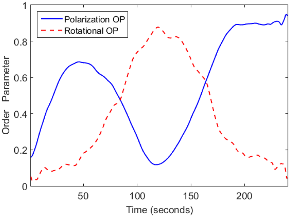
Polarization and rotational order parameters as a function of time for the experiment presented in Figure 3. At
Figure 3(a) shows our standard initial condition; seven robots placed in an hexagonal configuration where all interacting pairs are at the equilibrium distance
4.2. Stability analysis
In the experimental runs described above, we observed a phenomenon that was already apparent in the sinusoidal nature of Curve A in Figure 2; individual headings often display recurrent, persistent oscillations with respect to the mean heading direction after achieving translational collective motion. These oscillations can be seen, for example, in Videos SV1 and SV4 of the Supplementary Material. To understand the origins of this phenomenon, we carried out a simple linear stability analysis, which we detail below.
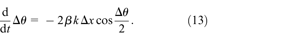
We consider a system of two robots advancing together side by side at the equilibrium distance
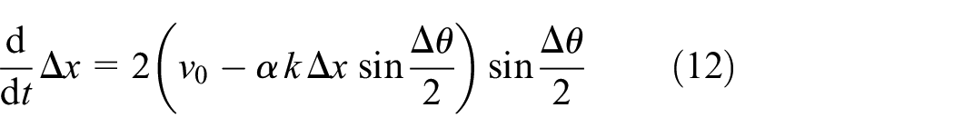
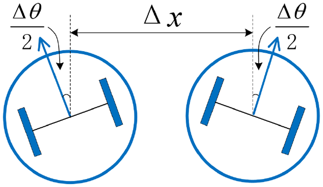
Sketch of the minimal two-robot fully symmetric setup for studying the linear stability of the aligned state. Perturbation variables
If we then linearize these expressions for small
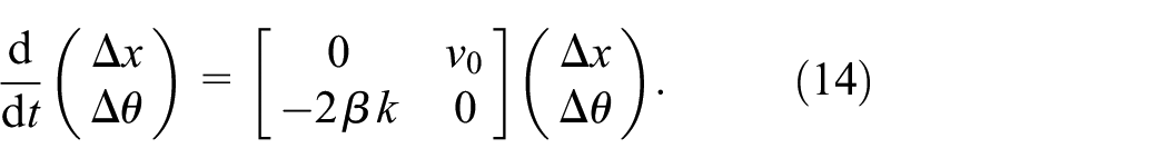
We can then compute the eigenvalues of the stability matrix in this equation, which are given by

Since both eigenvalues are purely imaginary, we conclude that this simple two-robot toy system displays marginal linear stability and that linear perturbations will not dampen out, producing instead persistent oscillations.
Although our experimental system contains many more degrees of freedom than the toy case described above, this analysis suggests that the AE control algorithm does not dampen out linear perturbations. Instead, it will sustain small oscillations that can only decay due to nonlinear interactions. This appears to explain the observed small, persistent heading oscillations, suggesting that the AE algorithm may have fundamental limitations in achieving and maintaining perfect alignment.
4.3. Experimental noise analysis
Our experimental control system can have multiple sources of error. We will refer to these, generically, as noise. An interesting advantage of our setup is that the information required by each agent to determine its next linear and angular speeds is measured and broadcasted simultaneously to all robots. This allows us to characterize the experimental noise by comparing their predicted and observed values at every update step.
Panel (a) of Figure 6 displays a scatter plot of the difference at every update step between predicted and observed angular and linear speed values, labeled
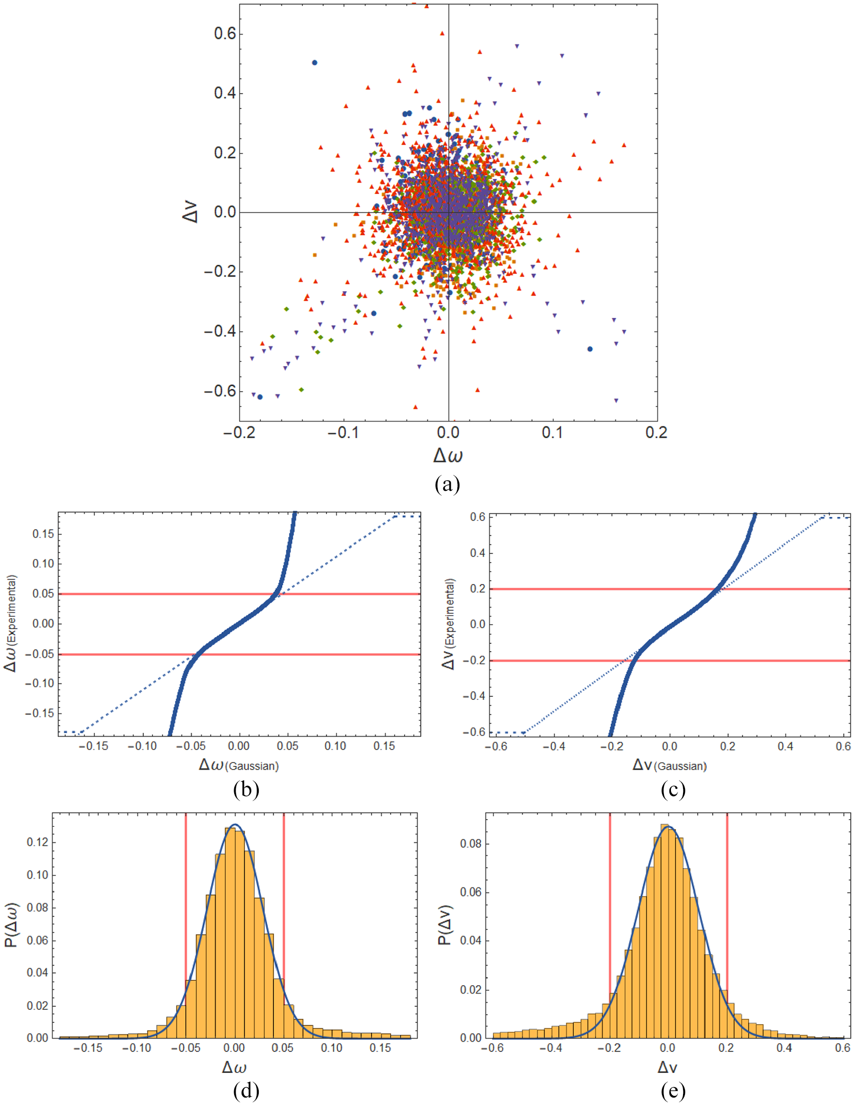
Analysis of the experimental noise in the angular and linear speeds of each robot. All plots display the difference between their predicted and measured values after every experimental update, labeled
Rather than attempting to capture all the subtleties of the experimental noise, we will focus here on finding a minimal description of the noise distribution that reproduces the main qualitative properties of the observed dynamics. We therefore search for Gaussian functions that match only the central regions of the
The analysis presented above shows that our noise distributions can be reasonably well approximated by Gaussian functions. We can therefore simulate the experimental noise by adding normally distributed random variables to the speed and angular velocity of each agent. We will implement this approach below to study how this noise and the control parameters affect self-organization.
5. Dependency on control parameters
In this section, we will study how the self-organizing dynamics and the stability of polarized states depend on the AE algorithm parameters
In order to reduce our parameter space to two dimensions, we will use the non dimensional quantities
The simulations implemented for this section were designed to closely mimic our experiments. In order to reproduce the effects of the experimental update step, we used a forward Euler method with numerical time-step
Following the approaches described above, we carried out a set of experimental and numerical runs using for the same parameter combinations, starting from our standard initial conditions, and mimicking numerically the experimental update step and noise. We characterize below the resulting dynamics and self-organizing properties.
5.1. Experimental and numerical dynamics
Figure 7 displays examples of the typical polarization order parameter dynamics
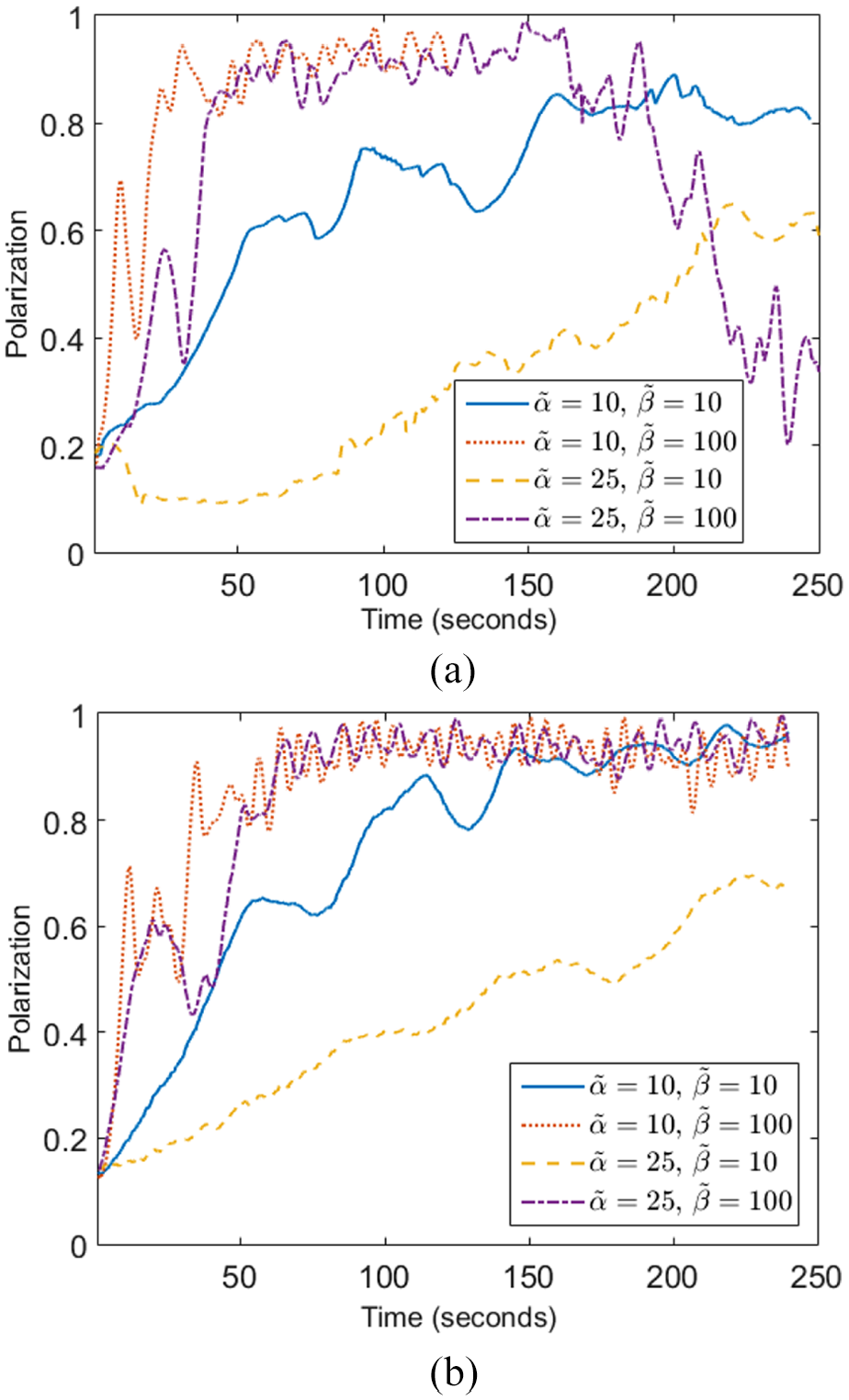
Polarization order parameter as a function of time for selected experimental and numerical runs with the same non-dimensional parameter combinations (
Time
Mean polarization
The figure shows that the experimental and numerical curves display similar features. For the same
We hypothesize that the difference that we observe between the experimental and numerical dynamics is mainly due to the long tails displayed by the noise distributions in Figure 6. These are not captured by our Gaussian approximations and reflect rare but strong perturbations that can push the swarm away from its ordered state. We note, however, that this difference could also be due to other properties of the noise not included in our model, such as systematic hardware errors or correlations between noise sources. In order to examine the potential role of these different factors in mimicking numerically the observed dynamics, future works will have to develop a more detailed description of the noise (including its systemic components for different specific hardware pieces and its multiple underlying correlations) and quantitative measures for characterizing the self-organizing dynamics of the specific robot swarm under consideration.
5.2. Phase diagrams
We will now study how self-organization into translating collective motion depends on the control parameters
We present below two phase diagrams, each corresponding to a different order parameter. The first-order parameter,
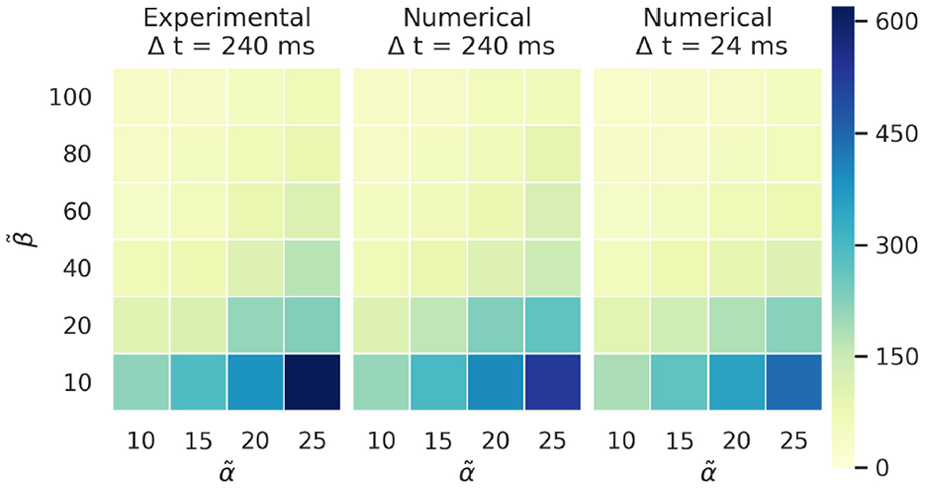
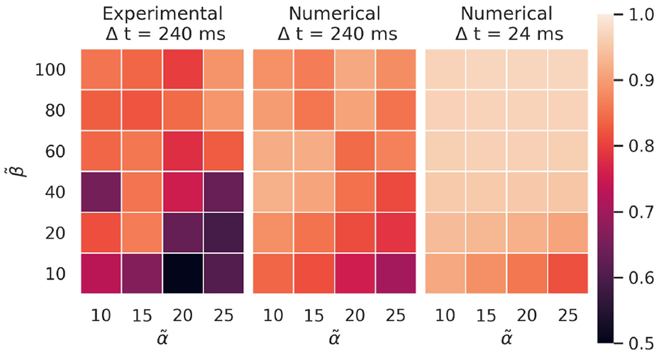
Figures 8 and 9 present the experimental and numerical phase diagrams for
The left-side panel of Figure 8 displays the mean value of
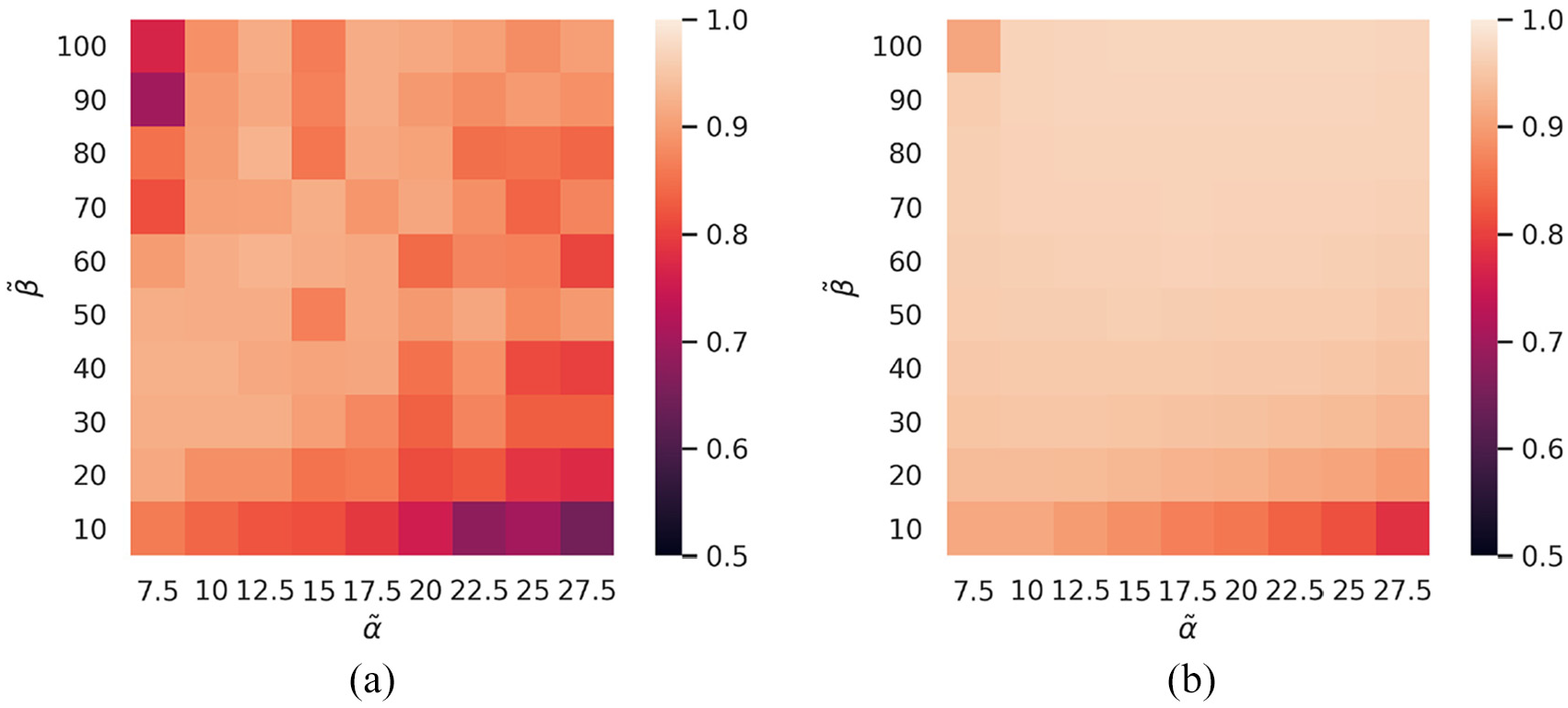
Figure 9 presents the mean value of
In order to better understand the structure of these phase diagrams and their dependency on
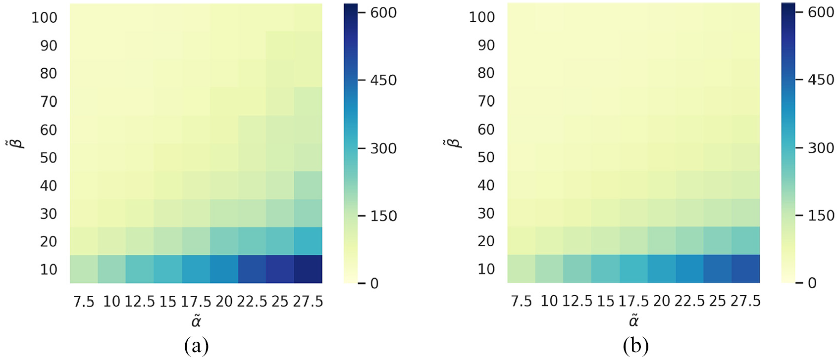
Time
Mean polarization
By combining the information in these types of phase diagrams, it is possible to predict the region of parameter combinations that should favor fast and robust self-organization in a given experimental system. After inspecting Figures 10 and 11, for example, we can estimate that in our specific setup,
6. Rotational collective motion
Collective rotation is another state of collective motion found in nature (Calovi et al., 2014; Pitcher, 1983; Radakov, 1973; Tunstrøm et al., 2013), in which agents self-organize to orbit around a central point. In this section, we will show that our AE algorithm can be modified to produce self-organization into this rotating state.
In order to achieve collective rotation, we made a small modification in the AE equations, introducing a different
We carried out proof-of-concept experiments to test whether real-world rotational collective motion can be achieved with our modified AE algorithm. We performed two sets of five repetitions of the experiments detailed below, always obtaining the same qualitative outcome. For these tests, we set up an elongated structure, rather than a hexagon, using the same seven robots. This structure increases the difference between the largest and smallest preferred
Figure 12 displays snapshots of our proof-of-concept experiment. As shown in Panel (a), all robots were initially placed at a distance
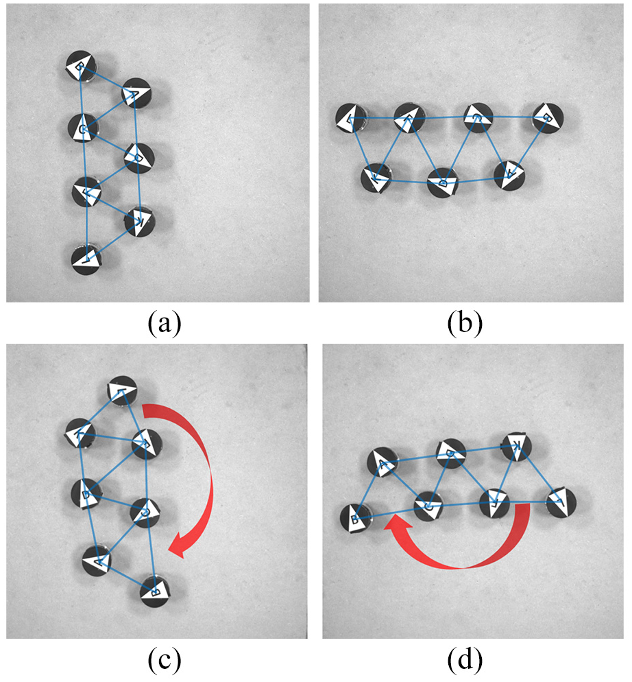
Snapshots of a proof-of-concept robot swarm experiment that self-organizes into rotational collective motion by following the control algorithm in Section 6 (see video SV5 in the Supplementary Material). The overlaid blue lines indicate which robots are interacting. (a) Initial condition with all robots at natural distance
The ability demonstrated above by our modified AE algorithm to self-organize agents into a rotating state highlights the many potential applications of our AE model in robot swarm control. Indeed, as discussed in the “Introduction” section, most decentralized control algorithms rely on explicit alignment, and can therefore only produce collective translation. The AE model will instead lead a group of agents to the lowest accessible elastic mode of their collective structure, which can be designed through small modifications to correspond to any number of collective states. For example, given that our elastic forces can be established permanently between any combination of robots (not only all nearest neighbors), one can imagine defining interaction networks that lead to self-organized states with various locally rotating substructures.
7. Discussion and conclusions
In this work, we have analyzed for the first time the capabilities and limitations of the AE model as a real-world decentralized control algorithm in a swarm robotics experiment. In contrast to its only previous implementation, in Ferrante et al. (2012), we focused here on characterizing the dependency of the self-organizing dynamics on model parameters and the effects of the experimental noise. We thus showed that it can effectively lead robots to self-organize into collective translating or rotating motion. Since the AE algorithm relies only on the positional information of neighbors, our experiments showed that robots do not require hardware that detects the headings of other robots to achieve self-organized collective motion.
Our control algorithm was fully implemented on board, but it was fed the robot’s own orientation and neighbor positions by an external tracking system set up above the arena. Despite its current use of external information, this implies that the AE algorithm could be executed fully autonomously in other robots, if they have sensors capable of determining this information individually and with enough precision. Note that, in this case, each robot would not require additional hardware to determine its own heading direction, since the position of its neighbors would already be measured with respect to the orientation of its own reference frame.
It is important to point out that a fully onboard implementation of the AE algorithm (including all sensing) would result in several differences when comparing with our experiments. The most notable practical difference is that no external position acquisition capabilities would be needed, thus allowing the implementation of the AE algorithm in a broader range of conditions. Regarding algorithm performance, the difference will depend on the precision and processing times of the onboard sensors when compared with our arena. On one hand, these sensors will typically be less precise than our external system, and could perform badly when confronted with occlusions or large inter-agent distances. On the other hand, our external system is based on image analysis, which has its own limitations. For example, the processing time is relatively long (and increases with the number of robots) and the position detection fails at the edges of the arena. The effects on noise and performance of using onboard sensors will thus depend on how they behave under the required operational conditions and for the desired swarm dynamics.
An important difference between onboard and external position acquisition systems that can be addressed in a general framework stems from the synchronous or asynchronous nature of their updating processes. Indeed, our arena acquisition system measures and broadcasts the required position information to all agents almost simultaneously. This implies that all robots update their control algorithms practically at the same time. In contrast, onboard sensors are typically not synchronized, so individual robot dynamics will be updated asynchronously. In order to test the effects of this difference, we performed preliminary simulations that show that the asynchronous and synchronous dynamics follow similar trends (data not shown). The asynchronous simulations appear to produce more noisy trajectories, however, especially in the high
The use of an external tracking system allowed us to study in detail the properties of the experimental noise. Indeed, the fact that the information required to execute the control algorithm is collected and broadcasted simultaneously to all robots makes our experiment equivalent to a numerical simulation with synchronous update. We are thus able to analyze the experimental noise by comparing the predicted and observed robot states after every time-step. We found that the noise distribution of both the angular and linear speeds can be well fitted by Gaussians. However, we also observed small deviations from this distribution in the form of long-tails that correspond to strong perturbations with low probability. Despite these differences, we were able to successfully model the effects of noise by adding to the linear and angular speed of each agent a Gaussian-distributed random variable with the corresponding, experimentally measured, standard deviation.
By simulating the effects of noise, we found that we can numerically predict the approximate dynamics observed in experiments. The speed of self-organization and the stability of the ordered states are slightly lower in experiments than in simulations, however, which is likely due to the observed non-Gaussian fluctuations and potential underlying correlations of the noise distributions. This could be verified in future work by using random variables with the exact experimental noise distributions. Despite these small differences, our results show that numerical simulations that approximately include the experimental noise can be used to determine the optimal operational regime of a real-world robot swarm.
We also found in this article that the AE algorithm produces a self-organized translating state in which robots display small persistent oscillations about the aligned state. We studied the source of these oscillations by carrying out a simple two-robot analytical calculation and showed that they are a generic feature of the AE control algorithm, resulting from the marginal linear stability of the aligned state.
Taken together, the results highlighted above suggest various ways in which our work could be generalized to other swarm robotic systems. First, our experimental analyses could be useful for the future implementation of position-based algorithms in any context where exchanging orientational information is impossible or inefficient (for example, if the robots have very limited sensing capabilities). Second, our studies lay the groundwork for extending this type of algorithms to other experimental robotic swarms, such as unmanned underwater or aerial vehicle swarms, since the AE model could be extended to three dimensions and to include the effects of inertia, winds, currents, and so on. Third, our characterization of the noise dynamics and of the response to parameter changes under real-world conditions could be generalized to other types of swarms. Fourth, we expect that an intermediate, compromise
In future work, we plan to further develop the noise characterization carried out in this article, in order to better match the theoretically predicted and the experimentally observed robot trajectories. We also plan to consider model modifications that could correct the marginal stability identified in the aligned state, which should improve its robustness. Furthermore, given that we demonstrated that rotational collective motion can be achieved by simply imposing different preferred speeds to different robots, we plan to test other simple modifications that could achieve new self-organized states, going beyond the usual collective translation or rotation. Finally, it would be interesting to extend our AE algorithm to three-dimensional systems, in order to test its effectiveness for Unmanned Aerial Vehicle (UAV) swarm control.
An interesting question that was not addressed in this article is how a group of robots that follow the AE algorithm would interact with obstacles. This is a complex matter, since the answer will strongly depend on their shape and their type of interactions with the robots. We can argue, however, that the AE algorithm has interesting potential capabilities in this regard. Indeed, since the model already includes attraction–repulsion forces, it provides a natural setting for designing different obstacle collision avoidance rules that can address specific swarm-obstacle interaction challenges. For example, if obstacles are treated as purely repulsive forces that are strong at short range but weak at intermediate (order
Supplemental Material
Supplemental Material
Supplemental Material
Supplemental Material
Supplemental Material
Footnotes
Acknowledgements
We are grateful for the help provided by Professor Zhongqi Sun (Beijing Institute of Technology) in implementing the Wi-Fi communication module that they designed and by Professor Lei Liu (University of Shanghai for Science and Technology) in debugging the tracking system.
Declaration of conflicting interests
The author(s) declared no potential conflicts of interest with respect to the research, authorship, and/or publication of this article.
Funding
The author(s) disclosed receipt of the following financial support for the research, authorship, and/or publication of this article: This work was supported by China National Natural Science Foundation (Grant No. 61374165) and China Scholarship Council (CSC) (Grant No. 201806040106).
Supplemental material
Supplemental material for this article is available online.
Notes
About the Authors
References
Supplementary Material
Please find the following supplemental material available below.
For Open Access articles published under a Creative Commons License, all supplemental material carries the same license as the article it is associated with.
For non-Open Access articles published, all supplemental material carries a non-exclusive license, and permission requests for re-use of supplemental material or any part of supplemental material shall be sent directly to the copyright owner as specified in the copyright notice associated with the article.