Investigating dominant situation of resting behavior as a potential labor pool in robotic swarm for group foraging

Abstract

The foraging task is a commonly studied scenario for distributed swarm robotic systems. The robots switch searching and resting behavior in a distributed manner to perform foraging quickly and energy efficiently. It is known that robots that are resting can act as a potential labor pool in addition to saving energy. Because they function as a potential labor pool, resting robots can help with foraging if needed. In this study, we consider the group foraging task, which requires two or more robots to transport a food item. In a group foraging task, resting robots can help with the transportation of a heavy food item in response to the recruitment of other robots. Until now, the efficacy of the resting behavior as a potential labor pool has been suggested, but the environments in which this function is dominant is still unknown. In this study, we propose a state-transition model for robots that includes the resting behavior and investigate the performance through multi-agent simulation. By comparing models with and without the resting behavior, we found that the function of the resting behavior as a potential labor pool is dominant in cases when the food items are heavy or the population is small.

Keywords

Task allocation group foraging recruitment swarm robotics

1. Introduction

A swarm robotic system (SRS) is composed of a swarm of robots that perform a given task faster than a single robot by actuating in different places simultaneously. Therefore, SRSs are expected to be used for several practical tasks such as warehousing (Digani et al., 2013), agriculture (Barrientos et al., 2011), and rescue activities (Kantor et al., 2006). In the design of a robot controller in a swarm, autonomous distributed control has attracted increasing attention in recent years (Bayindir, 2016). In autonomous distributed control, there is no central integrator, and each robot can access only local information. These limitations provide the robotic system with scalability, flexibility, and robustness.

The foraging task is a commonly studied scenario in SRSs as a model for real-world applications. In the foraging task, a specific area is designated as the nest and food items are scattered in the environment. The objective of the swarm is to discover the food items and then transport them to the nest. In addition, task allocation refers to the ability of each agent to dynamically change its task in a distributed manner (Hayakawa et al., 2020; Schmickl & Karsai, 2014). The challenge of SRS in the foraging task is to achieve task allocation such that the swarm of robots completes foraging quickly and energy efficiently.

Social insects allocate tasks for the foraging in a distributed manner, which inspired the solution for task allocation in SRSs. Wilson found that individual ants have a threshold they use to determine their response to a task (Wilson, 1984). Low-threshold resting ants become engaged in a task at a lower level of task-associated stimulus than high-threshold resting ants. In this way, the balance between the number of working and resting ants is dynamically adjusted in response to the environmental change. Based on this observation, the corresponding mathematical model, which is called the response threshold model, was constructed (Bonabeau et al., 1998).

The response threshold model has been used in foraging tasks for a swarm of robots. Task switching from resting to searching is represented using either probabilistic methods or threshold-based methods (Bayindir, 2016). In the following, we introduce both methods in solitary foraging scenarios in which each robot can transport a food item by itself. In probabilistic methods, each robot has a task switching probability, by which each robot switches its current task. Yang et al. give all robots an identical threshold value in the response threshold model (Yang et al., 2009). When food quantity inside the nest decreases, the task-associated stimulus increases. In that case, according to the response threshold model, some resting robots start searching for food items. In this way, food quantity inside the nest can be stabilized to a specific level. Castello et al. improved the response threshold model proposed by Yang et al. (2009) in such a way that each robot dynamically adjusts its personal threshold in response to the current stimulus (Castello et al., 2013). In a robot experiment, it was verified that the stability of the food quantity inside the nest was improved (Castello et al., 2016). Meanwhile, Labella et al. proposed another method to adjust the task switching probability (Labella et al., 2006). In this method, the probability increases in response to successful food retrieval, whereas the probability decreases when food retrieval fails. It was verified that this adaptation scheme contributes to energy-efficient foraging.

Meanwhile in threshold-based methods, each robot has a threshold value, and when a certain quantity reaches the corresponding threshold value, the robot always switches its task. Krieger and Billeter gave each robot a heterogeneous threshold value (Krieger & Billeter, 2000). When the energy level inside the nest is lower than the threshold of a resting robot, then the corresponding robot starts searching for food items. In this way, the food quantity inside the nest was stabilized to a specified level. Liu et al. dynamically changed the maximum resting and searching period of each robot in response to inter-robot collision, its own food retrieval result, and the food retrieval results of other robots (Liu et al., 2007). In detail, when each robot performs a resting (searching) behavior for the corresponding maximum resting (searching) period, then the robot switches its task. The adaptation of these periods improves the energy efficiency of foraging. Additionally, parameters related to the adaptation were optimized using genetic algorithms to maximize the net energy (Liu & Winfield, 2010).

Task allocation also has been studied for a foraging task consisting of sequentially dependent subtasks. A cache area, where the food items can be stored temporarily, is prepared between the food-searching area and the nest. Food items can be transferred from harvesting robots that search for food items to storing robots that transport the food items to the nest at the cache area indirectly. Following studies focus on task allocation between harvesting and storing to collect food items as much as possible. Pini et al. proposed the adaptive method for individual robots to decide whether to transport food items via the cache area by allocating the tasks or other long route (Pini et al., 2011, 2013). Brutschy et al. proposed the task switching rule based on the delay that the robots wait at the cache area (Brutschy et al., 2014). Lee et al. proposed the task switching rule such that adaptive task allocation is achieved under the mathematical guarantee (Lee et al., 2020). Ferrante et al. used an evolutionary algorithm to generate desirable task allocation of robots entirely from scratch (Ferrante et al., 2015).

The above studies assume solitary foraging scenarios. By contrast, group foraging is a foraging scenario in which the food item is so heavy that the cooperation of multiple robots is required to transport the food item. One application of group foraging in real life is human transportation in rescue missions (Gross et al., 2006). Group foraging is composed of a stage to gather a sufficient number of robots at the location of the food item and a stage to achieve cooperative transport. In the case of cooperative transport, robot controllers to achieve the desired velocity of the food item have been constructed (Farivarnejad et al., 2016; Wang & Schwager, 2016). Moreover, cooperative transport of ants has been analyzed (Berman et al., 2011; Feinerman et al., 2018) and emulated by swarm robotic systems (Wilson et al., 2018).

In the following, we summarize the robot controllers used in a swarm to perform the group foraging task including gathering of robots and cooperative transport. Fujisawa et al. constructed a state-transition model of robots by imitating ants, which lay pheromone trails (Fujisawa et al., 2014). In the state-transition model, all robots search for a food item without taking a rest. When one of the robots discovers a food item, it pushes the food item. If the food item cannot be transported due to a lack of power, then the robot lays a pheromone trail between the food item and the nest. When other searching robots perceive the trail, they travel toward the location of the food item along the trail. The above process is repeated until a sufficient number of robots have gathered at the location of the food item; thus, after a while, the robots can successfully transport the food item to the nest. Ijspeert et al. constructed a state-transition model for a stick pulling task which require cooperation of two robots (Ijspeert et al., 2001). In this study, heterogeneous gripping time parameter and inter-robot communication enhanced the number of successful stick pulling. Nouyan et al. constructed a state-transition model by which each robot serves as a landmark between the food item and the nest (Nouyan et al., 2009). By following the chain of the landmarks toward the food item, a sufficient number of robots have gathered at the location of the food item. Then, the robots can successfully transport the food item to the nest by following the chain toward the nest. On the other hand, when the robot serves as a landmark in the wrong place, it returns to the nest. The objective of the returning behavior is not resting but dissolving the wrong chain. Chen et al. focused on group foraging that the food item can occlude the robots’ perception of the goal location (Chen et al., 2015). When a robot performing a random walk has reached a food item, it moves such that the goal cannot be seen from the position. Then, it pushes the food item perpendicularly toward the food item’s surface in front of it. Based on this simple behavior, it was mathematically proved that the food item ultimately coincides with the goal. Jurt et al. constructed another state-transition model such that all robots search for an object without taking a rest (Jurt et al., 2022). When a sufficient number of robots are located at the object, then the robots agree on the timing of transportation. Alternatively, some robot behaviors for group foraging have been autonomously obtained using evolutionary computation (Yu et al., 2013) and deep reinforcement learning (Jin et al., 2020). Through learning, the robots acquire a behavior that causes them to gather together at the location of the food item without taking a rest. Then, they cooperatively transport the heavy food item. One limitation of computational learning methods based on neural networks is that neural networks are black-box systems, and therefore it is often very difficult to understand the behavior of these robots (Brambilla et al., 2013). As noted above (Chen et al., 2015; Fujisawa et al., 2014; Ijspeert et al., 2001; Jin et al., 2020; Jurt et al., 2022; Nouyan et al., 2009; Yu et al., 2013), several robot controllers have been proposed for group foraging. In those studies, energy efficiency was not evaluated, only task execution speed; thus, those controllers did not include a resting state.

However, in addition to saving energy, it is known that the resting behavior has the function of creating a potential labor pool. It can be beneficial to have a pool of resting workers available to take on larger tasks when they become available (Charbonneau & Dornhaus, 2015; Charbonneau et al., 2017) or to respond to a change in task demand (Radeva et al., 2017). Examples are as follows. In some ant species, when an ant discovers a food item outside the nest, it returns to the nest and actively recruits other ants inside the nest through antenna contact (Davidson et al., 2016). Those resting ants then start working and help retrieve the food item (Daly-Schveitzer et al., 2007; McCreery & Breed, 2014). In this way, these resting ants are exploited as a labor pool. Hayakawa et al. constructed a mathematical model of the life cycle of ants that allocates several tasks (Hayakawa et al., 2020). In the model, resting agents switch their task to another task that requires labor. Through simulation, it was verified that the task switching of the resting state improves the disturbance resistance of the colony. Hasegawa et al. used simulation to investigate the potential labor pool function of resting agents from the viewpoint of the sustainability of a colony (Hasegawa et al., 2016). The resting agents start working when the current workers become fatigued; thus, the resting agents perform the critical function of replacing workers. In this way, the agents process the task continuously as a swarm, and therefore the swarm obtains long-term sustainability.

As demonstrated in the above studies (Daly-Schveitzer et al., 2007; Hasegawa et al., 2016; Hayakawa et al., 2020; McCreery & Breed, 2014), the function of resting workers as a potential labor pool has been investigated in several ways. In group foraging, the resting behavior does not contribute to searching for food items, although it does function as a potential labor pool. However, state-transition models focusing on this function as a potential labor pool has not been constructed in terms of group foraging. Because of this, it is not fully understood when and how the resting behavior is effective in group foraging. In this study, we propose a robot state-transition model that includes the resting behavior. Using the state-transition model and multi-agent simulation, we investigate the situations in which the resting behavior functions as a potential labor pool and dominates performance.

The rest of this article is consisted as follows: Section 2 describes the problem setting, and Section 3 presents the proposed robot state-transition model. Section 4 presents the simulation setting, and Section 5 reports the simulation results. Section 6 concludes this article.

2. Problem setting

2.1. Environment

A field consists of a nest with a radius of r_N and a search area that are located concentrically on a two-dimensional plane (Figure 1(a)). The radius of the whole area is r_S. Global coordinate system is denoted by ∑_G ≡ (O − x y), whose origin O is set to the center of the nest and global axes x and y are fixed as shown in Figure 1(a). Initially, there are N_R robots, each with a radius of r_R, inside the nest and N_F food items, each with a radius of r_F, scattered in the search area. The purpose of the swarm of robots is to transport the food items to the nest quickly and energy efficiently. For each food item j, the weight is m, the angle from x-axis is denoted by ϕ_j, and distance from the center of the nest is denoted by d_j.

Figure 1.

Setting of the field and robot. (a) Field. (b) Side view of the robot. (c) Top view of the robot.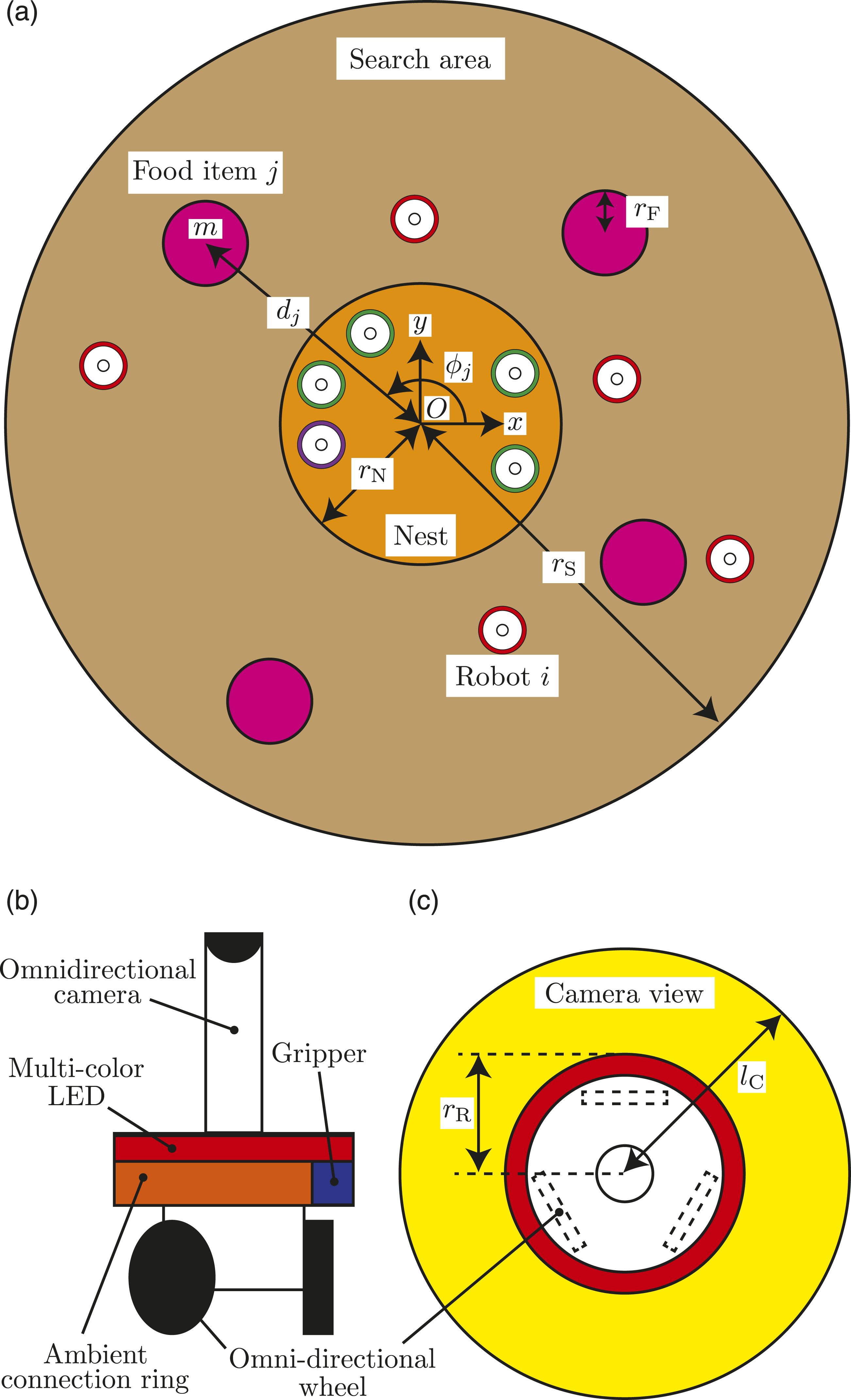

2.2. Robot specifications

In this study, the hardware and controllers of all robots are identical. There is no central integrator that comprehensively controls the robots; every robot autonomously determines its own behavior based on local information in a distributed manner. Each robot is equipped with the mobility such that the movement in any direction and the rotation on a two-dimensional plane are possible, for example, using three omnidirectional wheels (Yoshimoto et al., 2018) as shown in Figure 1(b).

Additionally, each robot is equipped with the following inexpensive and limited capabilities (Figure 1(b) and (c)):

• The robot can physically connect with another robot. For example, the robot is equipped with a passive ring around the body and an active gripper. The robot can grab the ring of another robot using the gripper so that they physically connect (Mondada et al., 2005).

• The robot can indicate the robot’s current state in the state-transition model, for example, using multi-color LEDs around the body (Mondada et al., 2005). The state-transition model includes at most nine states (see Section 3.3 in detail); thus, the difference between states can be indicated by changing the color.

• The robot can sense the position and state of neighboring robots and the position of neighboring food items, for example, using an omnidirectional camera with sensing distance l_C (Mondada et al., 2005). When a part of a food item or robot is inside the sensing area, then it can be sensed.

• The robot can measure the robot’s current position with respect to ∑_G, for example, using a light sensor and a compass. By indicating the nest position (i.e., the origin of ∑_G) using a light source, the robot can measure the nest position with respect to the robot coordinate using the light sensor (Fujisawa et al., 2014). Additionally, x and y directions can be measured by the compass (Zahugi et al., 2012).

2.3. Simulation model

In this study, to achieve the fast simulation under a large number of robots, we construct a custom-built multi-agent simulator. In the simulation, the position of the robot is determined based on the velocity input.

The dynamics of the food transportation is modeled as follows: When m or more robots push a food item in the same direction, then the corresponding food item is moved along with those robots.

Various collisions are modeled as follows: Let a “food-set” be a cluster composed of a food item and robots in direct contact with the food item or indirectly through other robots. Further, let a “bare-robot” be a robot that is not included in any food-set, and let a “wall” be an outer edge of the search area. When a food-set and bare-robot collide, the bare-robot behavior is consistent with that of the food-set because the weight of the food-set is very heavy. When two bare-robots collide, they do not move. When a bare-robot collides with a wall, the robot does not move. A collision between two food-sets is not considered because it is an unlikely situation. Other collisions between a food-set and wall or wall and wall do not occur in this study. A summary of the collision model is given in Table 1.

Table 1.

Collision Model. The Two Colliding Objects Are Shown Horizontally and Vertically. Repeated Combinations Are Indicated by Dashes.

Object	Object
Object	Food-set	Bare-robot	Wall
Food-set	Not consider	Consistent with the food-set	Not occur
Bare-robot	-	Stop	Stop
Wall	-	-	Not occur

3. Robot controller

We propose a robot controller for group foraging that includes the resting behavior. For the controller, we combine a conventional state-transition model of SRSs for solitary foraging (Liu et al., 2007) and an ant recruiting behavior for group foraging (Daly-Schveitzer et al., 2007).

3.1. Conventional state-transition model for solitary foraging

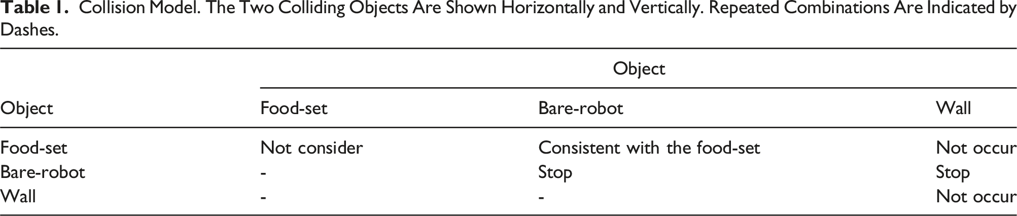
First, we introduce a state-transition model of the SRS that includes the resting behavior for solitary foraging. Figure 2 shows the state-transition model, which simplifies the threshold-based robot controller in Liu et al. (2007).

Figure 2.

State-transition model for solitary foraging, which is a simplified version of the model proposed by Liu et al. (2007). The upper part in each box shows the state and lower part shows the behavior.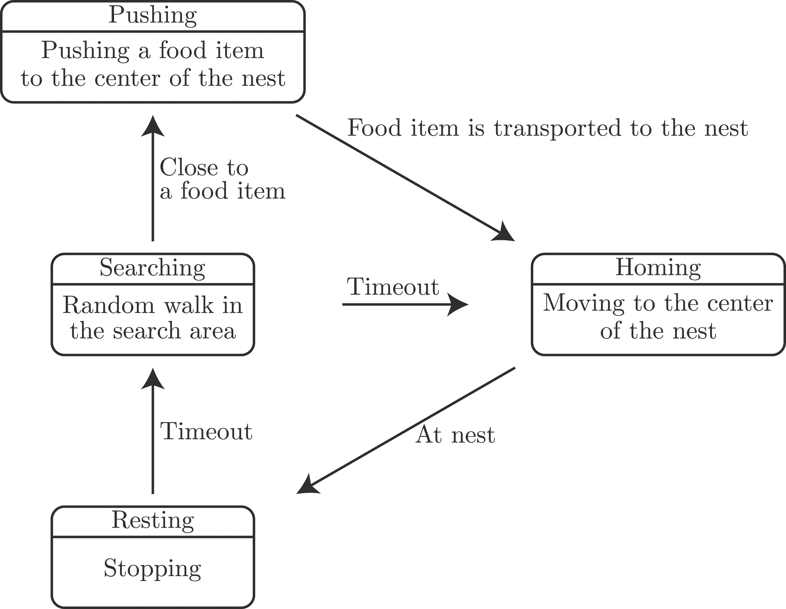

Next, we describe in detail the state-transition model.

Resting: Each robot in the Resting state is located in the nest and does not move. If sufficient time has passed, the robot changes its state from Resting to Searching.

Searching: Each robot in the Searching state performs a random walk in the search area and searches for food items that are not being transported. If a robot in the Searching state discovers a food item that is not being transported, it approaches the food item. After approaching, the robot changes its state from Searching to Pushing. If sufficient time has passed without finding a food item, the robot gives up searching and changes its state from Searching to Homing.

Pushing: Each robot in the Pushing state pushes the food item toward the center of the nest. If the food item enters the nest, the robot changes its state from Pushing to Homing.

Homing: Each robot in the Homing state moves to the center of the nest without pushing a food item. If the robot arrives at the nest, the robot changes its state from Homing to Resting.

In the above transition flow, robots in the Searching and Resting states exist simultaneously. By optimizing the timeout parameters, energy-efficient foraging can be achieved under several food density and population conditions (Liu et al., 2007).

3.2. Ant recruiting behavior for group foraging

Next, we introduce the recruiting behavior of the ant species Gnamptogenys sulcata (Daly-Schveitzer et al., 2007). When an ant discovers a food item (we call this ant the “finder”), the finder tries to transport the food item by itself. If the food item is light enough for the finder to transport, the finder transports the food item by itself. In this case, the foraging is equivalent to solitary foraging. By contrast, if the food item is so heavy that the finder cannot transport it, the finder returns to the nest while laying a chemical trail. After alerting its nestmates, the finder remarks the chemical trail back to the location of the food item. Because of this recruitment, a certain number of nestmates in the nest start to work and move toward the location of the food item by following the chemical trail that the finder has laid. Then, the following ants cooperatively try to transport the food item. If they still cannot transport the food item, the finder returns to the nest and recruits nestmates again. This process is repeated until the total number of ants located at the food item becomes sufficient; thus, the ants finally transport the food item.

3.3. Proposed state-transition model for group foraging

We extend the state-transition model for solitary foraging including the resting behavior (see Section 3.1) to a model for group foraging by adding the ant recruiting behavior (see Section 3.2). Figure 3 shows the proposed state-transition model for group foraging. When the food item is light enough for one robot to transport, then the robot behavior in Figure 3 (black and green states and transitions) is consistent with that for solitary foraging in Figure 2.

Figure 3.

Proposed state-transition model for group foraging. The upper part in each box shows the state and lower part shows the behavior. The green state represents the initial state of robots. Red states and transitions are newly added to the state-transition model for solitary foraging shown in Figure 2.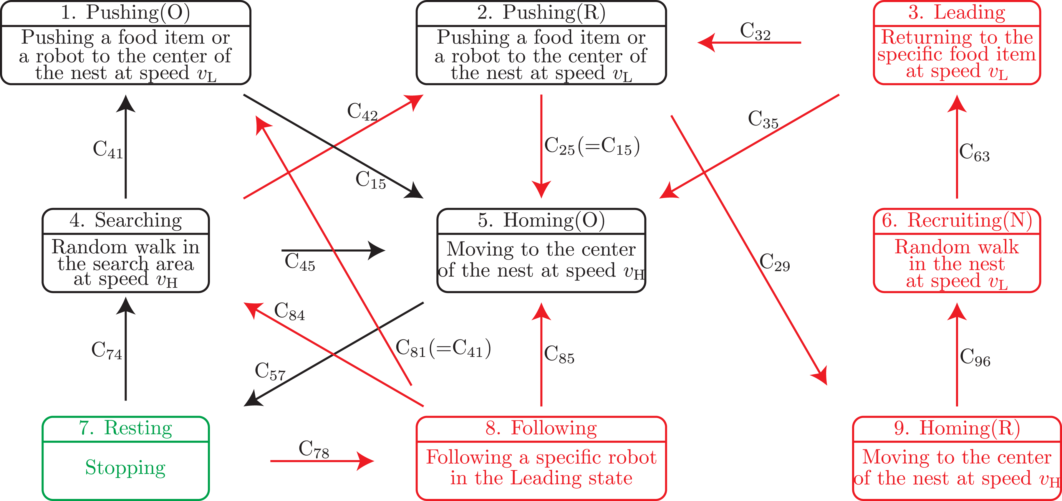

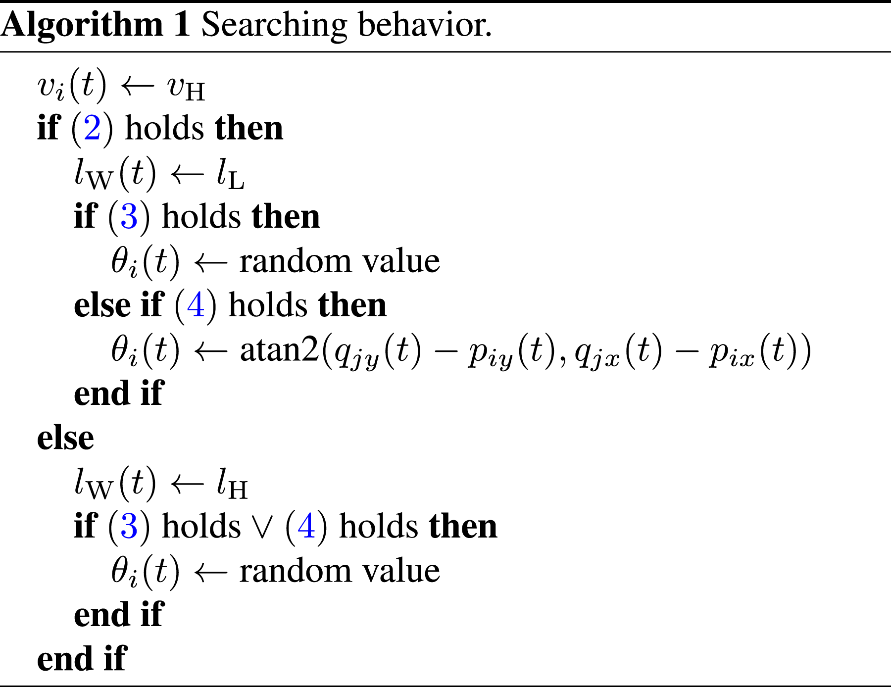
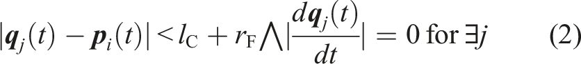
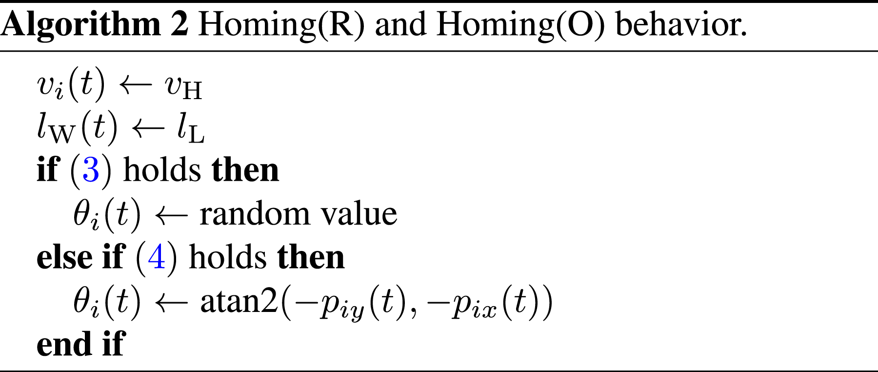
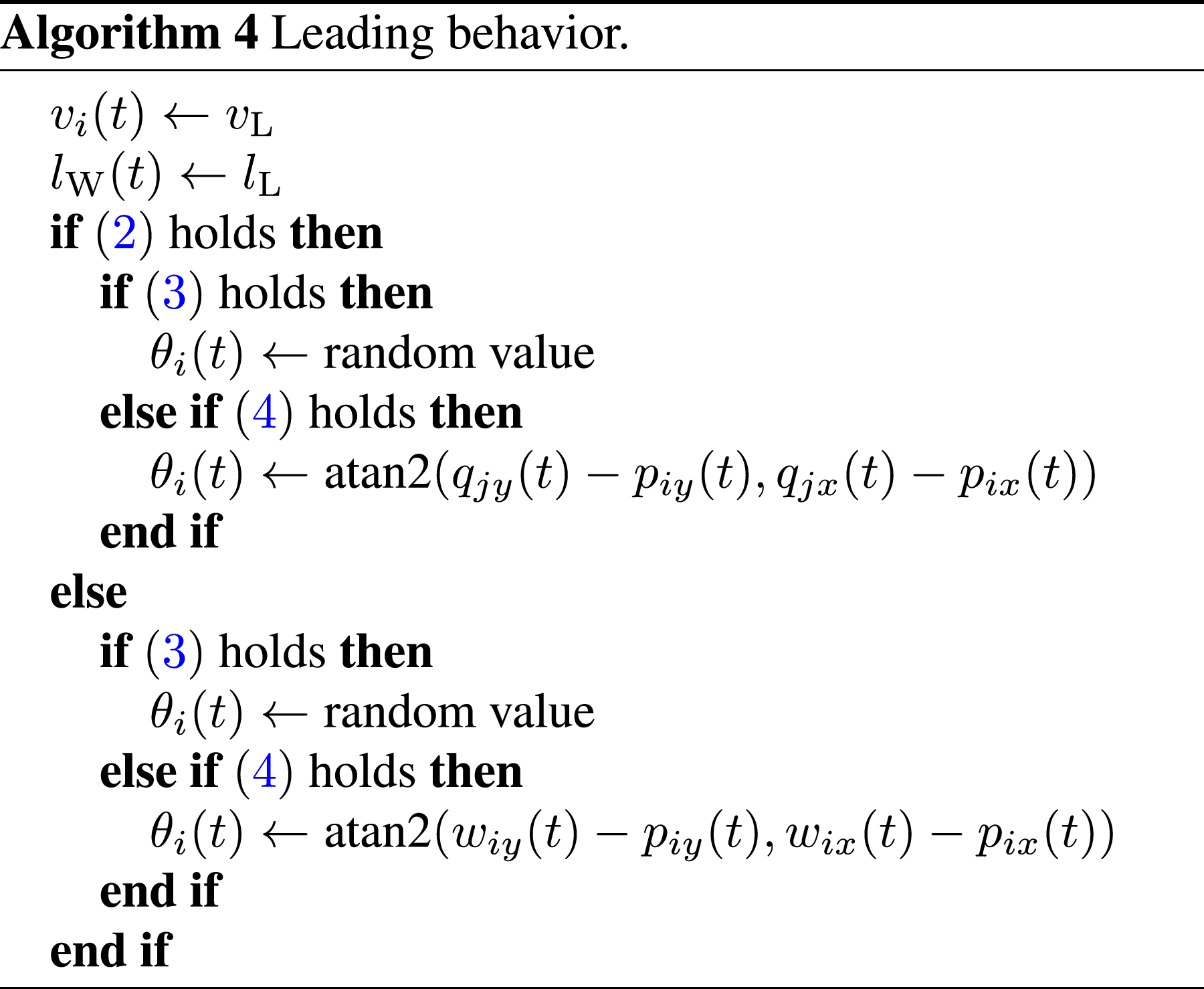
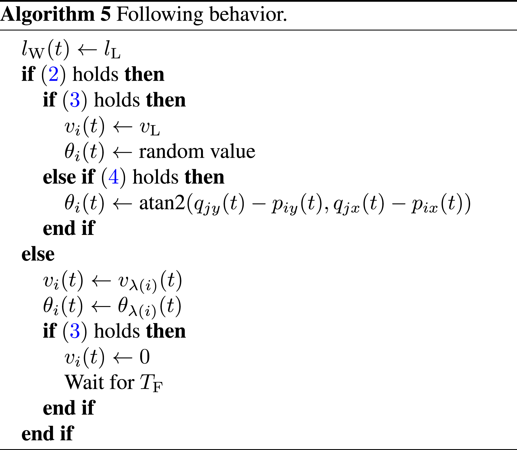
In the following, we explain the behavior and transition model of each state. All symbols representing a position are seen from ∑_G and symbols representing a direction are seen from x-axis. Let $p_{i} (t) \equiv {[p_{i x} (t) p_{i y} (t)]}^{T}$ and $q_{j} (t) \equiv {[q_{j x} (t) q_{j y} (t)]}^{T}$ be the two-dimensional position of the center of robot i and food item j at time t, respectively. Let v_i(t) be the target moving speed of robot i at time t, and let θ_i(t) be the target moving direction of robot i at time t, and let Θ_i(t) be ${[\cos θ_{i} (t) \sin θ_{i} (t)]}^{T}$ . Therefore, the position of robot i is calculated as follows:

p_{i} (t + Δ t) = p_{i} (t) + v_{i} (t) Δ t Θ_{i} (t) + u_{i} (t),

(1)

where Δt is the time step for updating the position of all robots and u _i(t) is the effect from environment, such as collision and food-pushing. Based on the collision and food-pushing effect, the robot position is passively adjusted as mentioned in Section 2.3. In this way, by determining the velocity input (i.e., v_i(t) and θ_i(t)), the position of all robots is determined. The robot behavior of each state is summarized as follows:

Resting: Each robot in the Resting state is located in the nest and does not move, that is, v_i(t) = 0.

Searching: Each robot in the Searching state performs a random walk in the search area at speed v_H. If a robot in the Searching state discovers a food item that is still not being transported, it approaches the food item.

To clarify the behavior of the robot, we define the following conditions (2)–(4).

| q_{j} (t) - p_{i} (t) | < l_{C} + r_{F} \land | \frac{d q_{j} (t)}{d t} | = 0 for \exists j

(2)

| u_{i} (t - Δ t) | > 0

(3)

Move l_{W} (t) continuously without changing θ_{i} (t)

(4)

(2) means that there is a food item within the camera’s field of view under the condition that the food item is not being transported. (3) means that a collision occurs in the previous time step. When (3) holds, then the robot changes its moving direction randomly. (4) means that the robot moves a sufficient distance continuously toward a specific direction, where l_W(t) corresponds to the mean free path of the random walk at time t. After a robot moves l_W(t), the robot changes its moving direction. When the robot searches for food items, l_W(t) is set to a large distance l_H. However, when the robot approaches the found food item, the robot aims at moving toward a specific place (i.e., the found food item); thus, l_W(t) is set to a small distance l_L only for resolving inter-robot collision. v_i(t) and θ_i(t) are determined in accordance with Algorithm 1, where in the initial state, θ_i(t) is set to a random value. In Algorithm 1, the behavior of the robots that do not enter the nest is omitted to simplify Algorithm 1. The value atan2(y, x) ∈ [0 2π) is atan(y/x) with its quadrant using two parameters x and y.

Pushing(R) and Pushing(O): A state with (R) represents a state of a finder robot for each food item which performs the recruiting behavior, whereas a state with (O) represents a state of other robot. Pushing(R) and Pushing(O) state differ in the next state-transition of robots, but the behaviors in both states are same. Each robot in the Pushing state (Pushing(R) or Pushing(O) state) pushes the food item or another robot that is grabbed with its gripper in the direction of the center of the nest at speed v_L. The robots in the Pushing state align their moving directions such that the center of the food item moves toward the center of the nest. Let σ(i) be the index of a food item which robot i pushes. Then, v_i(t) = v_L and θ_i(t) = atan2(−q_σ(i)y(t), − q_σ(i)x(t)).

Homing(R) and Homing(O): Homing(R) and Homing(O) state differ in the next state-transition of robots, but the behaviors in both states are same. Each robot in the Homing state (Homing(R) or Homing(O) state) moves to the center of the nest at speed v_H without pushing a food item. v_i(t) and θ_i(t) are determined in accordance with Algorithm 2, where in the initial state, θ_i(t) is set to atan2(−p_iy(t), − p_ix(t)).

Recruiting(N): Each robot in the Recruiting(N) state performs a random walk in the nest at speed v_L. It moves without actively attracting other robots; thus, it does not count the number of robots that follow it. v_i(t) and θ_i(t) are determined in accordance with Algorithm 3. In the initial state, θ_i(t) is set to the previous one (i.e., θ_i(t − Δt)) so that the robot approaches the center of the nest for recruiting. In Algorithm 3, the behavior of the robots that do not enter the search area is omitted to simplify Algorithm 3.

Leading: Each robot in the Leading state moves straight toward location of the found food item which is stored in its memory at speed v_L. Let $w_{i} (t) \equiv {[w_{i x} (t) w_{i y} (t)]}^{T}$ be the two-dimensional position of the center of the food item in the memory of robot i. v_i(t) and θ_i(t) are determined in accordance with Algorithm 4, where in the initial state, θ_i(t) is set to atan2(w_iy(t) − p_iy(t), w_ix(t) − p_ix(t)).

Following: Each robot in the Following state matches its velocity to the velocity of the recruiting robot that triggered the state-transition from Resting to Following. This behavior corresponds to velocity matching in Boids (Reynolds, 1987). In this following behavior, there is no collision between the robots that follow the same leading robot. When a collision occurs between a following robot and another robot, the following robot stops so that the collision avoidance behavior does not influence the other following robots much. After a short time T_F has passed, the another robot would move to resolve the collision; thus, the following robot starts to follow the leading robot again. Let the index of the robot that is being followed by robot i be λ(i). v_i(t) and θ_i(t) are determined in accordance with Algorithm 5.

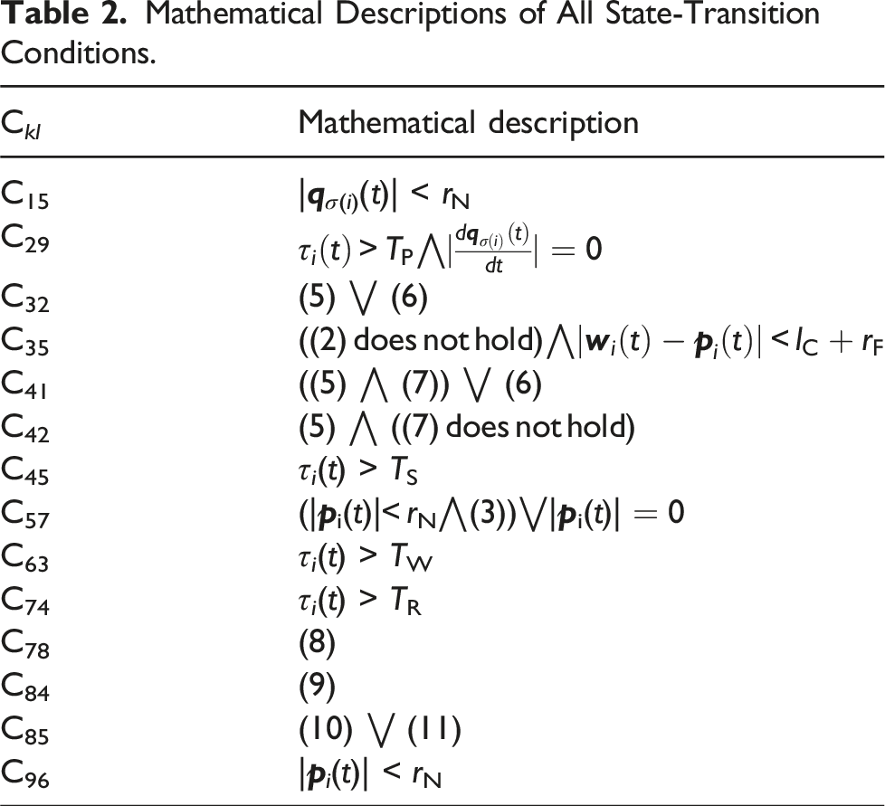
Let C_kl be a state-transition condition in the proposed model from state k to state l, as shown in Figure 3. Let τ_i(t) be the duration robot i has been operating in its current state at time t. Duration τ_i(t) increases as time goes by and is reset to 0 when robot i changes its state to another state. Let T_R, T_S, T_P, and T_W be the maximum durations of resting, searching, pushing, and recruiting, respectively. In the initial state, all robots are located randomly within the nest and set to the Resting state such that the τ_i(0) for each robot i is set randomly within the range [0 T_R]. The state-transition model of each state is summarized as follows:

C₁₅: The center of the transporting food item enters the nest area, that is, | q _σ(i)(t)| < r_N.

C₂₉: τ_i(t) > T_P holds under the condition that the food item is not being transported, that is, $| \frac{d q_{σ (i)} (t)}{d t} | = 0$ .

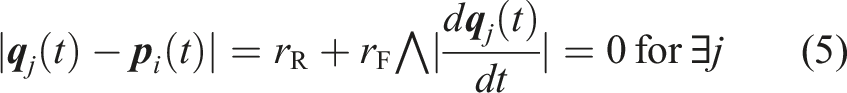
C₃₂: The robot is close to a food item that is not being transported. Alternatively, the robot is close to another robot in the Pushing(O) state under the condition that a food item that is not being transported is within the camera’s field of view. Here, Pushing(R) state is excluded because the robot in the Pushing(R) state moves away from the food item in a short time for recruitment. Let I_s(t) be an index set of robots whose state is s at time t. To clarify the state-transition condition, we define the following conditions (5) and (6).

| q_{j} (t) - p_{i} (t) | = r_{R} + r_{F} \land | \frac{d q_{j} (t)}{d t} | = 0 for \exists j

(5)

(2) \land | p_{k} (t) - p_{i} (t) | = 2 r_{R} for \exists k \in I_{Pushing (O)} (t)

(6)

(5) means that there is a food item which is contacting to the robot under the condition that the food item is not being transported. (6) means that there is a robot in the Pushing(O) state that is contacting to the robot. C₃₂ is equivalent to the condition of (5) ∨ (6).

C₃₅: There is no food item that is not being transported within the camera’s field of view under the condition that the robot has returned to the position of the found food item, which is stored in its memory. In other words, (2) does not hold under the condition that | w _i(t) − p _i(t)| < l_C + r_F holds.

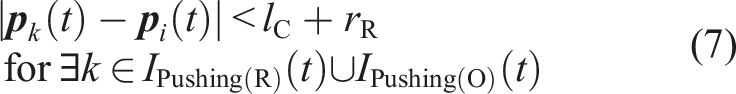
C₄₁: The robot is close to a food item that is not being transported under the condition that another pushing(R) or Pushing(O) robot is within the camera’s field of view. Alternatively, the robot is close to another robot in the Pushing(O) state under the condition that a food item that is not being transported is within the camera’s field of view. To clarify the state-transition condition, we define the following condition (7).

\begin{aligned} | p_{k} (t) - p_{i} (t) | < l_{C} + r_{R} \\ for \exists k \in I_{Pushing (R)} (t) \cup I_{Pushing (O)} (t) \end{aligned}

(7)

(7) means that there is a robot in the Pushing(R) or Pushing(O) state within the camera’s field of view. C₄₁ is equivalent to the condition of ((5)∧(7))∨(6).

C₄₂: The robot is close to a food item that is not being transported under the condition that no other robot in the Pushing(R) or Pushing(O) state is within the camera’s field of view. In other words, (5) holds under the condition that (7) does not hold.

C₄₅: τ_i(t) > T_S holds.

C₅₇: The robot collides with another robot under the condition that the center of the robot has entered the nest area. Alternatively, the center of the robot reaches the center of the nest. In other words, (| p _i(t)|< r_N∧(3))∨| p _i(t)| $= 0$ .

C₆₃: τ_i(t) > T_W holds.

C₇₄: τ_i(t) > T_R holds.

C₇₈: Another robot in the Recruiting(N) state is within the camera’s field of view. C₇₈ is equivalent to the following condition (8).

| p_{k} (t) - p_{i} (t) | < l_{C} + r_{R} for \exists k \in I_{Recruiting (N)} (t),

(8)

where (8) means that there is a robot in the Recruiting(N) state within the camera’s field of view.

C₈₄: The robot that is being followed is within the camera’s field of view and transits its state to Pushing(R). C₈₄ is equivalent to the following condition (9).

| p_{λ (i)} (t) - p_{i} (t) | < l_{C} + r_{R} \land λ (i) \in I_{Pushing (R)} (t),

(9)

where (9) means that there is a followed robot within the camera’s field of view under the condition that the followed robot’s state is Pushing(R).

C₈₅: The robot that is being followed is within the camera’s field of view and transits its state to Homing(O). Alternatively, the robot that is being followed is outside the camera’s field of view. To clarify the state-transition condition, we define the following conditions (10) and (11).

| p_{λ (i)} (t) - p_{i} (t) | < l_{C} + r_{R} \land λ (i) \in I_{Homing (O)} (t)

(10)

| p_{λ (i)} (t) - p_{i} (t) | \geq l_{C} + r_{R},

(11)

where (10) means that there is a followed robot within the camera’s field of view under the condition that the followed robot’s state is Homing(O). (11) means that the followed robot does not exist within the camera’s field of view. C₈₅ is equivalent to the condition of (10) ∨ (11).

C₉₆: The center of the robot enters the nest area, that is, | p _i(t)| < r_N.

All the above state-transition conditions are summarized in Table 2.

Table 2.

Mathematical Descriptions of All State-Transition Conditions.

C_kl	Mathematical description
C₁₅	\| q _σ(i)(t)\| < r_N
C₂₉	$τ_{i} (t) > T_{P} \land \| \frac{d q_{σ (i)} (t)}{d t} \| = 0$
C₃₂	(5) ∨ (6)
C₃₅	((2) does not hold) $\land \| w_{i} (t) - p_{i} (t) \| < l_{C} + r_{F}$
C₄₁	((5) ∧ (7)) ∨ (6)
C₄₂	(5) ∧ ((7) does not hold)
C₄₅	τ_i(t) > T_S
C₅₇	(\| p _i(t)\|< r_N∧(3))∨\| p _i(t)\| $= 0$
C₆₃	τ_i(t) > T_W
C₇₄	τ_i(t) > T_R
C₇₈	(8)
C₈₄	(9)
C₈₅	(10) ∨ (11)
C₉₆	\| p _i(t)\| < r_N

As shown in Section 3.2, a finder ant first returns to the nest, then performs recruiting for a certain period, and then returns to the food item. This single cycle of the recruiting behavior corresponds to the following flow: Searching $\underset{C_{42}}{˗}$ Pushing(R) $\underset{C_{29}}{\to}$ Homing(R) $\underset{C_{96}}{\to}$ Recruiting(N) $\underset{C_{63}}{\to}$ Leading. This cycle from the Pushing(R) to Leading states is repeated until the food item has been transported (i.e., C₁₅ holds).

Meanwhile, a resting ant follows a finder ant, reaches the food item, and then pushes the food item as part of the additional labor pool. The following behavior corresponds to the following flow: Resting $\underset{C_{78}}{\to}$ Following $\underset{C_{41}}{\to}$ Pushing(O).

In this way, by repeating the recruiting behavior, the total number of robots that are located at the found food item increases.

4. Simulation setting

We verified the efficacy of the proposed state-transition model for group foraging through multi-agent simulation. In the simulation, the foraging performance of the proposed state-transition model with the resting behavior and another conventional model without the resting behavior was compared.

4.1. Conventional state-transition model without resting for comparison

As explained in Section 1, the conventional robot controllers for group foraging do not include a resting state (Chen et al., 2015; Fujisawa et al., 2014; Ijspeert et al., 2001; Jin et al., 2020; Jurt et al., 2022; Nouyan et al., 2009; Yu et al., 2013). In accordance with those previous studies, we newly constructed a state-transition model without resting and homing states, as shown in Figure 4 for comparison. In the following, we call the state-transition model in Figure 3 the proposed model, whereas the state-transition model in Figure 4 is called the conventional model.

Figure 4.

State-transition model for group foraging without a resting state. The upper part in each box shows the state and lower part shows the behavior. The green state represents the initial state of robots. Red state and transitions correspond to the modified parts of the proposed model in Figure 3. C_kl is common to Figure 3.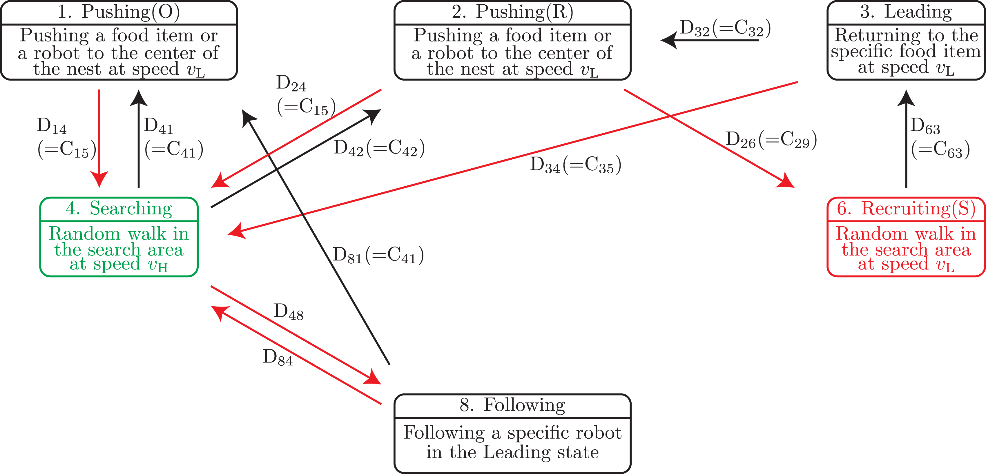

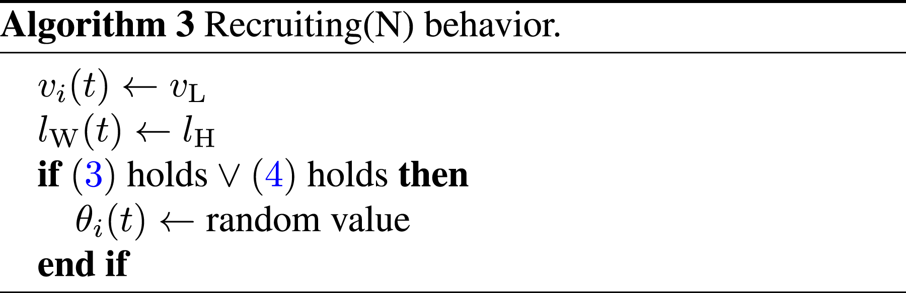
In the initial state, all robots are located randomly within the nest and set to the Searching state. Because the conventional model has no resting behavior, a finder robot recruits other robots in the Searching state, which are located in the search area. Additionally, because the resting behavior has been eliminated, the Recruiting(S) state is newly defined. Each robot in the Recruiting(S) state performs a random walk as shown in Algorithm 3 in the search area instead of the nest area.

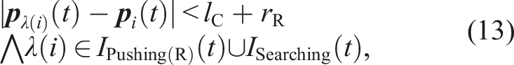
Let D_kl be a state-transition condition in the conventional model from state k to state l, as shown in Figure 4. The state-transition conditions are as follows:

D₄₈: Another robot in the Recruiting(S) state is within the camera’s field of view. D₄₈ is equivalent to the following condition (12).

| p_{k} (t) - p_{i} (t) | < l_{C} + r_{R} for \exists k \in I_{Recruiting (S)} (t),

(12)

where (12) means that there is a robot in the Recruiting(S) state within the camera’s field of view.

D₈₄: The robot that is being followed is within the camera’s field of view and transits its state to Pushing(R) or Searching. Alternatively, the robot that is being followed is outside the camera’s field of view. To clarify the state-transition condition, we define the following condition (13).

\begin{aligned} | p_{λ (i)} (t) - p_{i} (t) | < l_{C} + r_{R} \\ \land λ (i) \in I_{Pushing (R)} (t) \cup I_{Searching} (t), \end{aligned}

(13)

where (13) means that there is a followed robot within the camera’s field of view under the condition that the followed robot’s state is Pushing(R) or Searching. D₈₄ is equivalent to the condition of (11) ∨ (13).

4.2. Initial state of the food items

Let the total weight of all food items scattered in the field be m_total. The weight of each food item m is set to m_total/N_F in such a way that the weight of the food items decreases as the number of food items increases; thus, the total number of robots required to transport all N_F food items simultaneously is constant. As a result, there are a few heavy food items when N_F is small, whereas there are many light food items when N_F is large. A figure showing the influence of changing m_total is uploaded as a supplemental material. Additionally, the ϕ_j for each food item j is randomly determined.

Next, we set the distance between each food item j and center of the nest, that is, d_j. When d_j is large, it is difficult to discover food item j and it takes much time to transport this food item to the nest. We determined d_j such that the difficulty of transporting all food items is constant regardless of N_F as follows: d_j is given randomly within search area [r_N + r_F r_S − r_F] such that $\sum_{j = 1}^{N_{F}} m d_{j} = W$ holds, where W is a constant value.

4.3. Evaluation method of foraging performance

We evaluated the performance of a swarm based on the food transport rate and energy efficiency. Let N_T be the total number of food items that are located inside the nest at the end of the simulation. The food transport rate of the swarm of robots is defined by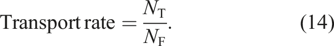

Transport rate = \frac{N_{T}}{N_{F}} .

(14)

Next, we define energy efficiency. Regarding energy consumption, a robot in the Resting state does not consume energy because it does not move, whereas a robot in all other states consumes energy at one unit per time step because it is always moving or pushing a food item. The total consumed energy of robot i in the simulation is denoted by e_i and regarded as the cost. The total weight of the transported food items is regarded as the reward. From Labella et al. (2006), the energy efficiency of a swarm of robots is defined as the ratio of reward to cost as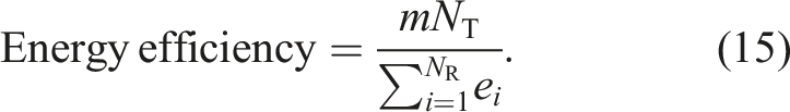

Energy efficiency = \frac{m N_{T}}{\sum_{i = 1}^{N_{R}} e_{i}} .

(15)

4.4. Other settings

The simulation ended when all food items were transported to the nest or 2000 s elapsed. The food items which were transported to the nest were removed at the moment. To evaluate the foraging performance in various scenarios, the total number of robots (i.e., N_R) and total number of food items (i.e., N_F) were set to various values. Moreover, parameter T_W (i.e., recruiting period) influences the performance. Therefore, for both the proposed and conventional models, we changed T_W from 10 s to 1000 s in 10 s increments. Moreover, the initial positions of the robots and random walk behavior include randomness, and hence we repeated the simulation 10 times for each T_W to investigate the average performance for both models. All constant parameters for the robots and environment are summarized in Table 3.

Table 3.

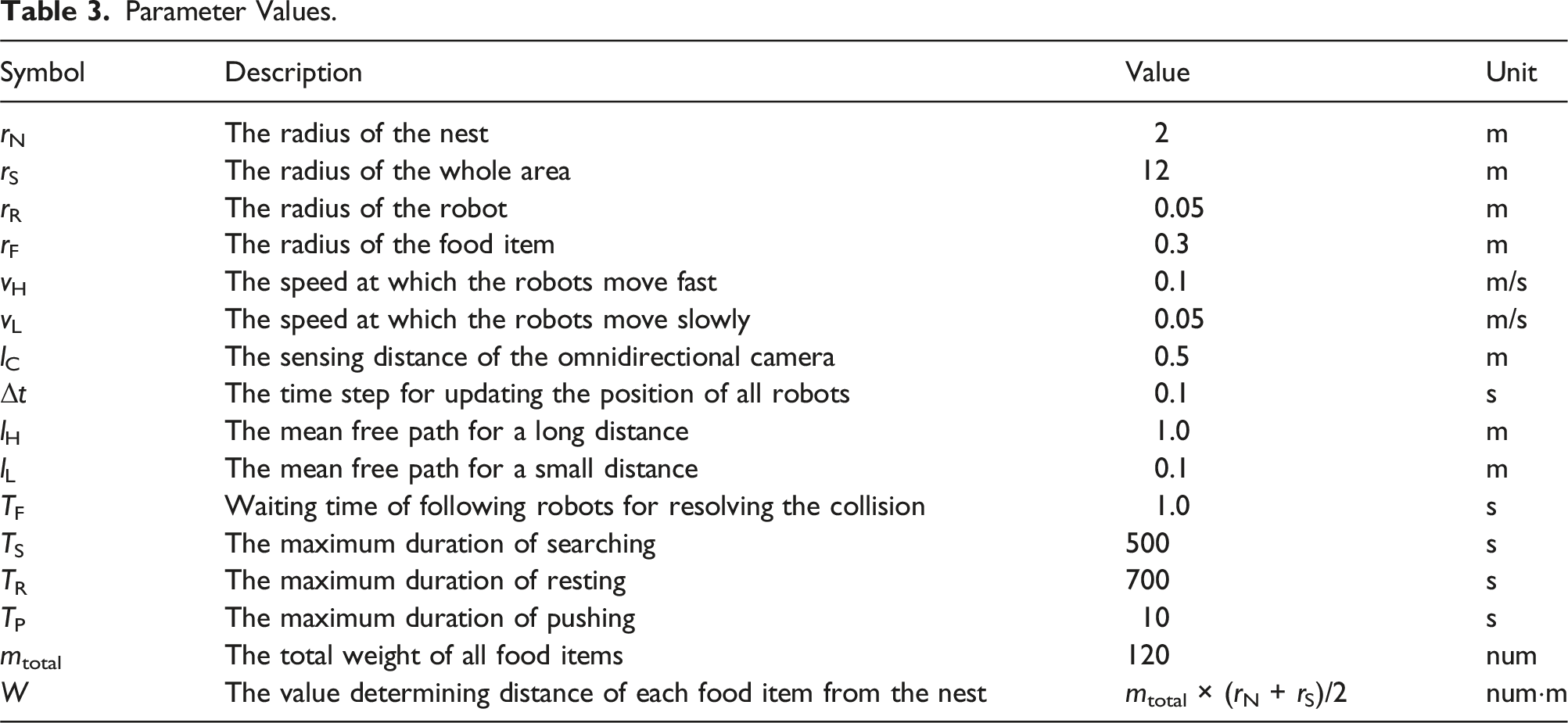
Parameter Values.

Symbol	Description	Value	Unit
r _N	The radius of the nest	2	m
r _S	The radius of the whole area	12	m
r _R	The radius of the robot	0.05	m
r _F	The radius of the food item	0.3	m
v _H	The speed at which the robots move fast	0.1	m/s
v _L	The speed at which the robots move slowly	0.05	m/s
l _C	The sensing distance of the omnidirectional camera	0.5	m
Δt	The time step for updating the position of all robots	0.1	s
l _H	The mean free path for a long distance	1.0	m
l _L	The mean free path for a small distance	0.1	m
T _F	Waiting time of following robots for resolving the collision	1.0	s
T _S	The maximum duration of searching	500	s
T _R	The maximum duration of resting	700	s
T _P	The maximum duration of pushing	10	s
m _total	The total weight of all food items	120	num
W	The value determining distance of each food item from the nest	m_total × (r_N + r_S)/2	num⋅m

5. Simulation result and discussion

5.1. Visualization of the robot behaviors in both models

First, we visualize the robot behaviors in both models in one of the simulations. Figure 5 visualizes the multi-agent simulation for the case of (N_R, N_F, T_W) = (100, 6, 100) in the proposed model. When a robot in the Searching state discovers a food item (Figure 5(b)), the robot pushes the food item toward the center of the nest. Because the robot fails to transport it because of a lack of power, the finder robot starts to return to the nest (Figure 5(c)). After the finder robot has arrived at the nest, the finder robot transits to the Recruiting(N) state and recruits other resting robots in the nest (Figure 5(d)). Some robots in the Resting state find the recruiting robot and then transit to the Following state (Figure 5(e)). After a sufficient time has passed while recruiting, the finder robot transits to the Leading state and leads the following robots to the location of the food item (Figure 5(f)). After the finder robot has reached the location of the food item, the robots that followed the finder start to push or search for the corresponding food item (Figure 5(g)). Some of the searching robots successfully discover the corresponding food item and transit to the Pushing(O) state (Figure 5(h)). Thus, the total number of robots in Pushing state at the location of the food item increases. This recruiting process is repeated by finder robots as long as the corresponding food item is not being transported. Finally, a sufficient number of robots in the Pushing state are located at the position of the corresponding food item, and then the food item is transported by those robots (Figure 5(i)).

Figure 5.

Visualization of the multi-agent simulation for the case of (N_R, N_F, T_W) = (100, 6, 100) in the proposed model. Red characters represent the behavior of the recruiting robots, whereas blue characters represent the behavior of the following robots. (a) t = 0 s. Initial state. (b) t = 87 s. A robot discovers a food item. (c) t = 97 s. The finder starts to return to the nest because of the shortage of pushing robots. (d) t = 121 s. The finder starts to recruit other robots inside the nest. (e) t = 130 s. Some resting robots start to follow the finder. (f) t = 221 s. The finder starts to lead the following robots to the location of the corresponding food item. (g) t = 274 s. The finder reaches the location of the corresponding food item. The robots that followed the finder start to search for the corresponding food item or push it. (h) t = 289 s. The robots that followed the finder successfully found the corresponding food item and start to push the food item. On the other hand, the finder robot started to return to the nest again because of the shortage of pushing robots. (i) t = 439 s. Finally, the corresponding food item is transported.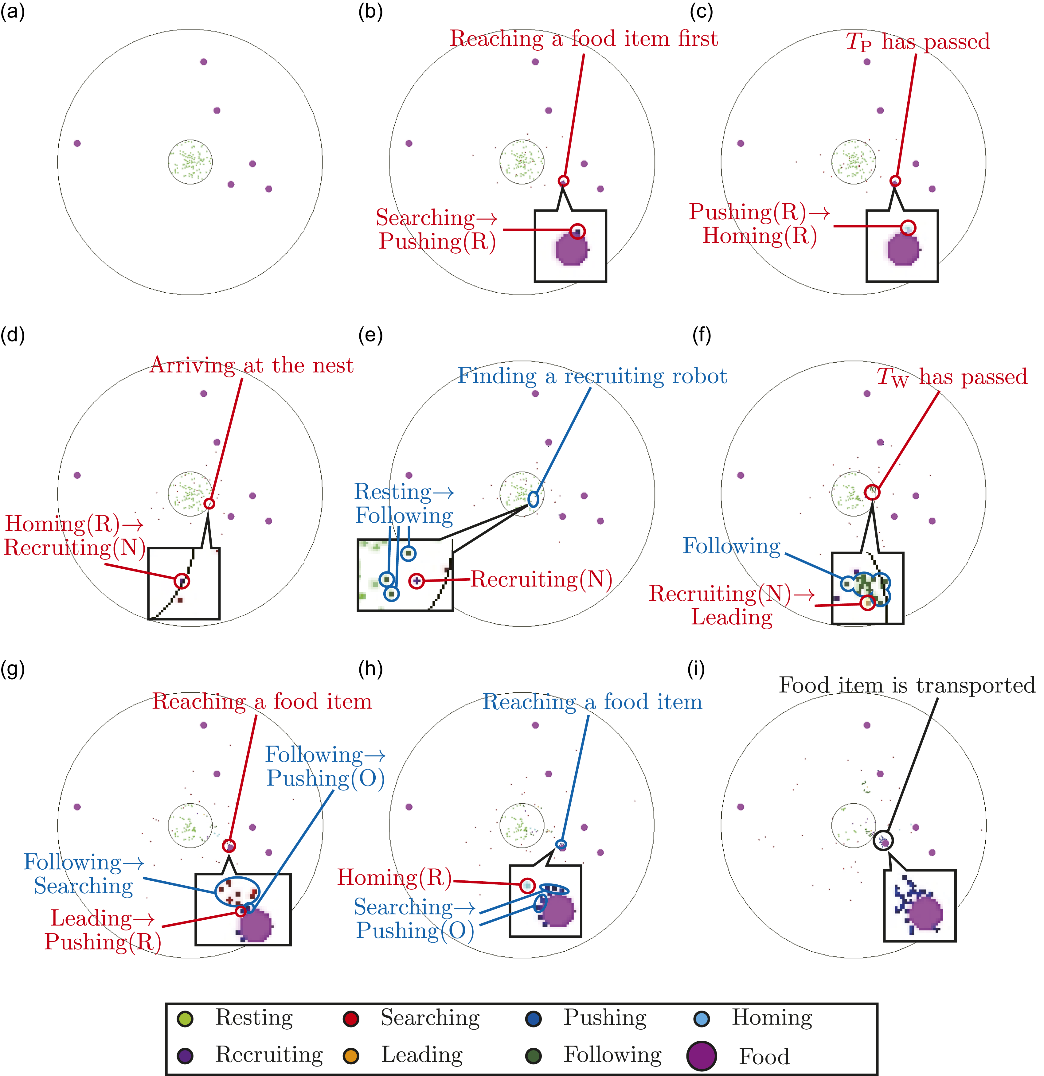

Meanwhile, Figure 6 visualizes the multi-agent simulation for the case of (N_R, N_F, T_W) = (100, 6, 100) in the conventional model. In the conventional model, all robots search for food items, so it takes less time to discover a food item than in the proposed model (Figure 6(b)). Because the robot fails to transport it because of a lack of power, the finder robot starts to recruit other searching robots in the search area (Figure 6(c)). Some robots in the Searching state find the recruiting robot and then transit to the Following state (Figure 6(d)). After a sufficient time has passed while recruiting, the finder robot transits to the Leading state and leads the following robots to the location of the food item (Figure 6(e)). After the finder robot has reached the location of the food item, the robots that followed the finder start to push or search for the corresponding food item (Figure 6(f)). Because the number of robots that followed the finder is small, the total number of robots which start pushing is fewer than in the proposed case (Figure 6(g)). This recruiting process is repeated by finder robots as long as the corresponding food item is not being transported. Finally, a sufficient number of robots in the Pushing state are located at the corresponding food item’s position, but it takes more time to gather the pushing robots at the location of the food item than in the proposed model (Figure 6(h)). Two videos showing whole simulation about Figures 5 and 6 are uploaded as supplemental materials.

Figure 6.

Visualization of multi-agent simulation for (N_R, N_F, T_W) = (100, 6, 100) in the conventional model. Red characters represent the behavior of the recruiting robots, whereas blue characters represent the behavior of the following robots. (a) t = 0 s. Initial state. (b) t = 25 s. A robot discovers a food item. (c) t = 35 s. The finder starts to recruit other robots in the search area because of the shortage of pushing robots. (d) t = 63 s. Some searching robots start to follow the finder. (e) t = 135 s. The finder starts to lead the following robots to the location of the corresponding food item. (f) t = 177 s. The finder reaches the location of the corresponding food item. The robots that followed the finder start to search for the corresponding food item or push it. (g) t = 187 s. The finder robot starts to recruit other robots again because of the shortage of pushing robots. On the other hand, one of the robots that followed the finder still searches for the corresponding food item. (h) t = 1047 s. Finally, the corresponding food item is transported.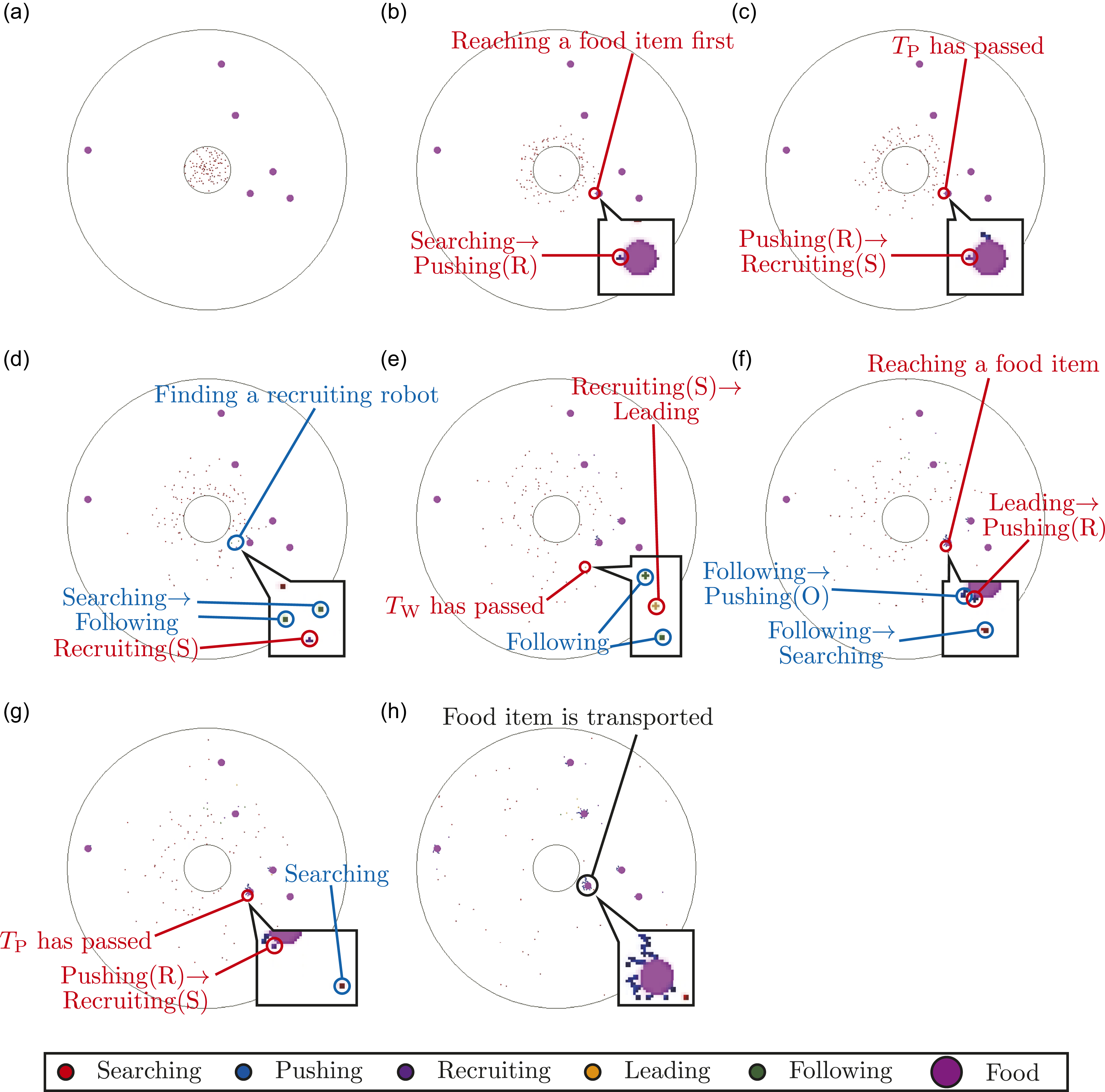

5.2. Comparison of the models with respect to the number of food items

Next, we evaluate the performance of the proposed and conventional models in various environments. We prepared four scenarios such that N_R was set to 100 and N_F was set to 6, 8, 10, 12.

5.2.1. Quantitative evaluation of the model performances

First, we compared the food transport rate. Figure 7 shows the average transport rate and energy efficiency for the two models in several environments. We call the T_W value that maximizes the transport rate the optimal T_W. The value of T_W can be arbitrary selected; thus, it is reasonable to evaluate the performance when T_W is the optimal value. Figure 7 shows that the proposed strategy induces the highest transport rate around T_W = 100 for all N_F. By contrast, the conventional strategy achieves almost the same transport rate regardless of T_W for all N_F. As N_F increases, the food transport rate of the proposed model remains almost constant, whereas that of the conventional model increases. When each food item is heavy, for instance, N_F = 6 and 8, the maximum transport rate of the proposed model is higher than that of the conventional model (Figure 7). As a result, we found that the small N_F environment is a situation in which the resting behavior dominates. In these situations, the advantage of the potential labor pool created by the resting behavior exceeds the disadvantage of doing nothing.

Figure 7.

Average transport rates and energy efficiencies with different T_W over 10 runs under various N_F and N_R = 100. Shaded areas indicate the standard deviation. The average differences under the optimal T_W were examined using a two-sided independent sample t test. Here, ∗ indicates a significance level of 0.01 for the two optimal values of T_W.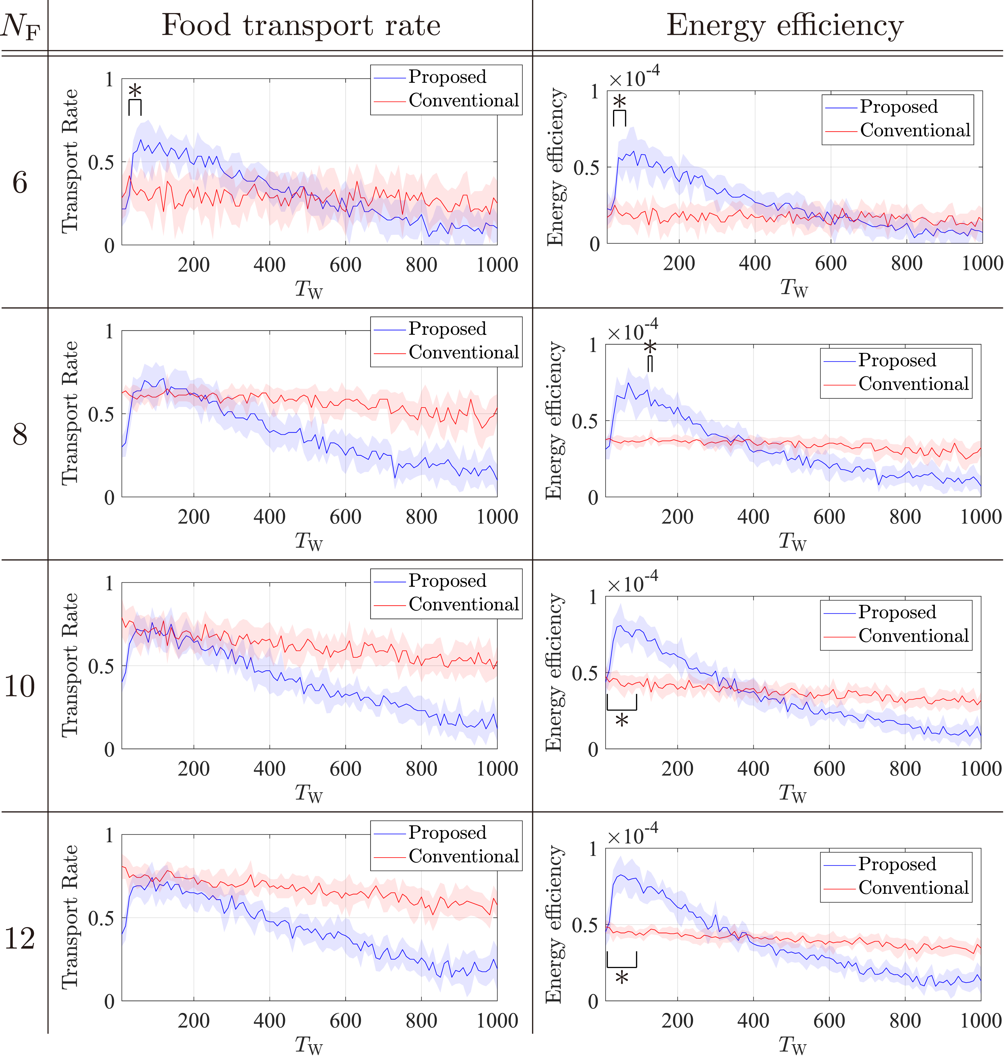

Next, we compared the energy efficiency. As shown in Figure 7, the values of T_W that maximizes the transport rate and energy efficiency are almost the same. Therefore, the maximum energy efficiency can also be evaluated when the optimal value of T_W is used. Figure 7 reveals that the proposed model outperforms the conventional model in maximum energy efficiency for all environments. This is because the resting robots help foraging only if needed; thus, they generally save energy.

5.2.2. Reasons for the performance differences

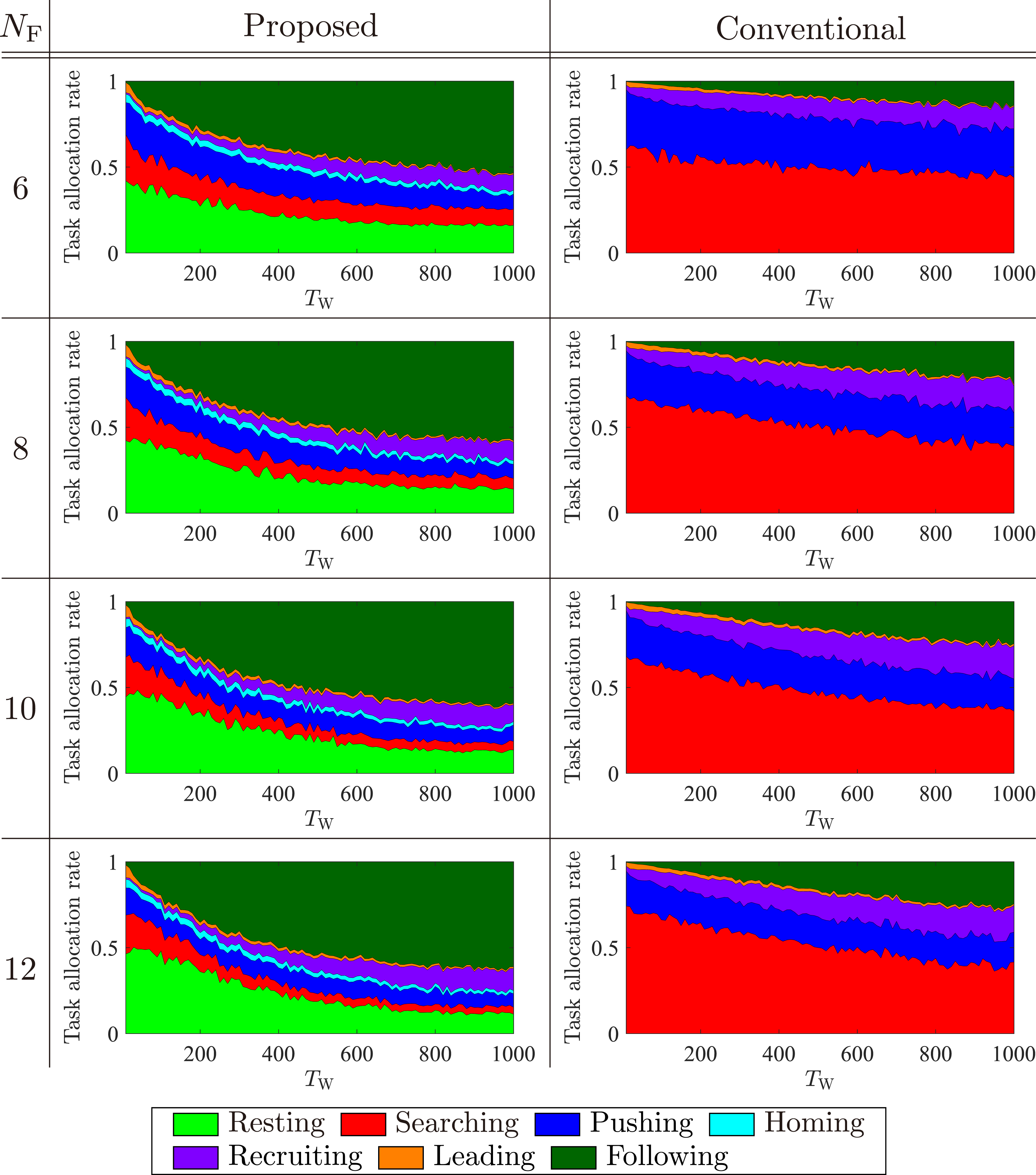
Next, we discuss the reasons for the performance differences in various environments. To investigate these reasons, we focused on the task allocation rate. Let N_k(t) be the number of robots whose state is k at time t. Furthermore, let total period of each simulation be T_sim. We denote the average task allocation rate for each task k in one simulation by A_k, which is represented as

A_{k} = \frac{\sum_{t = 1}^{T_{sim}} N_{k} (t)}{T_{sim} N_{R}} .

(16)

Figure 8 shows the average task allocation rates for the proposed and conventional models.

Figure 8.

Average task allocation rates for the proposed and conventional models with different T_W over 10 runs under various N_F and N_R = 100.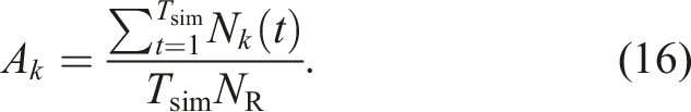

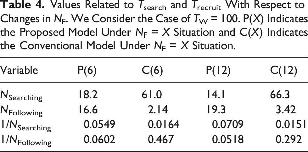
Let T_tot be the duration from the start of the simulation to the moment at which sufficient number of robots has been gathered for a food item. Let T_search be the duration of searching for the food item and T_recruit be the duration of recruiting a sufficient number of robots. T_tot is the sum of T_search and T_recruit as follows:

T_{tot} = T_{search} + T_{recruit} .

(17)

When the robots in the Searching state are spatially distributed in the search area, the probability of finding a food item is proportional to N_Searching. Therefore, T_search ∝ 1/N_Searching.

Additionally, T_recruit is equivalent to the duration needed to gather m or more robots at the food item. When the robots in the Following state are spatially distributed to each food item, the number of following robots for a specific food item is in proportion to N_Following/N_F. Therefore, T_recruit ∝ mN_F/N_Following. Furthermore, considering that mN_F is constant, T_recruit ∝ 1/N_Following.

Table 4 summarizes N_Searching and N_Following of both models in the two cases of N_F, which are obtained by the results in Figure 8. Table 4 reveals that 1/N_Following in the conventional model is 0.467 in N_F = 6 and 0.292 in N_F = 12, respectively. As a result, T_recruit in the conventional model dramatically decreases as N_F increases. This is because the increase in N_F induces an increase in the recruiting robots. However, T_search in both models and T_recruit in the proposed model do not change much, even if N_F increases. Therefore, as N_F increases, only the food transport rate of the conventional model increases (Figure 7). Hence, we can understand the reason why the small N_F environment is a situation in which the resting behavior dominates.

Table 4.

Values Related to T_search and T_recruit With Respect to Changes in N_F. We Consider the Case of T_W = 100. P(X) Indicates the Proposed Model Under N_F = X Situation and C(X) Indicates the Conventional Model Under N_F = X Situation.

Variable	P(6)	C(6)	P(12)	C(12)
N _Searching	18.2	61.0	14.1	66.3
N _Following	16.6	2.14	19.3	3.42
1/N_Searching	0.0549	0.0164	0.0709	0.0151
1/N_Following	0.0602	0.467	0.0518	0.292

Additionally, we explain the reason why the proposed model has more following robots than the conventional model (Figure 8). In the proposed model, recruiting robots recruit resting robots inside the nest, whereas those in the conventional model recruit searching robots in the search area. The average density of robots that can start following in the proposed model is $N_{R} A_{Resting} / π r_{N}^{2} = N_{R} \cdot A_{Resting} / (π \cdot 4)$ and that in the conventional model is $N_{R} A_{Searching} / π (r_{S}^{2} - r_{N}^{2}) = N_{R} \cdot A_{Searching} / (π \cdot 140)$ . Moreover, from Figure 8, the ratio of A_Searching in the conventional model to A_Resting in the proposed model is always smaller than 4. Therefore, the average density of robots that can start following in the proposed model is always larger than that in the conventional model. It is known that the performance of the swarm is influenced by the density of its agents (Hamann, 2013; Hunt et al., 2019), which is in accordance with the efficacy of the recruitment in this study.

5.3. Comparison of the models with respect to population

Next, we compared the performance of the models when number of robots was varied. We prepared four scenarios such that N_R was set to 70, 100, 130, 160 and N_F was set to 6.

5.3.1 Quantitative evaluation of the model performances

Figure 9 shows the average transport rate and average energy efficiency for the two models in several population sizes. Figure 9 reveals that the proposed strategy induces the highest transport rate around T_W = 100 for all N_R. By contrast, the conventional strategy induces almost the same transport rate regardless of the value of T_W for all N_R. This result is consistent with the change in the number of food items described in Section 5.2.1. As N_R increases, the food transport rate of the proposed model increases a little, whereas that of the conventional model increases dramatically. When N_R is small, that is, N_R = 70, 100, and 130, the maximum transport rate of the proposed model is higher than that of the conventional model (Figure 9). As a result, we found that small N_R environment is a situation in which the resting behavior dominates. In such situations, the advantage of the potential labor pool function of the resting behavior exceeds the disadvantage of doing nothing.

Figure 9.

Average transport rates and energy efficiencies with different values of T_W over 10 runs under N_F = 6 and various N_R. Shaded areas indicate the standard deviation. The average differences under the optimal T_W were examined using a two-sided independent sample t test. Here, ∗ indicates a significance level of 0.01.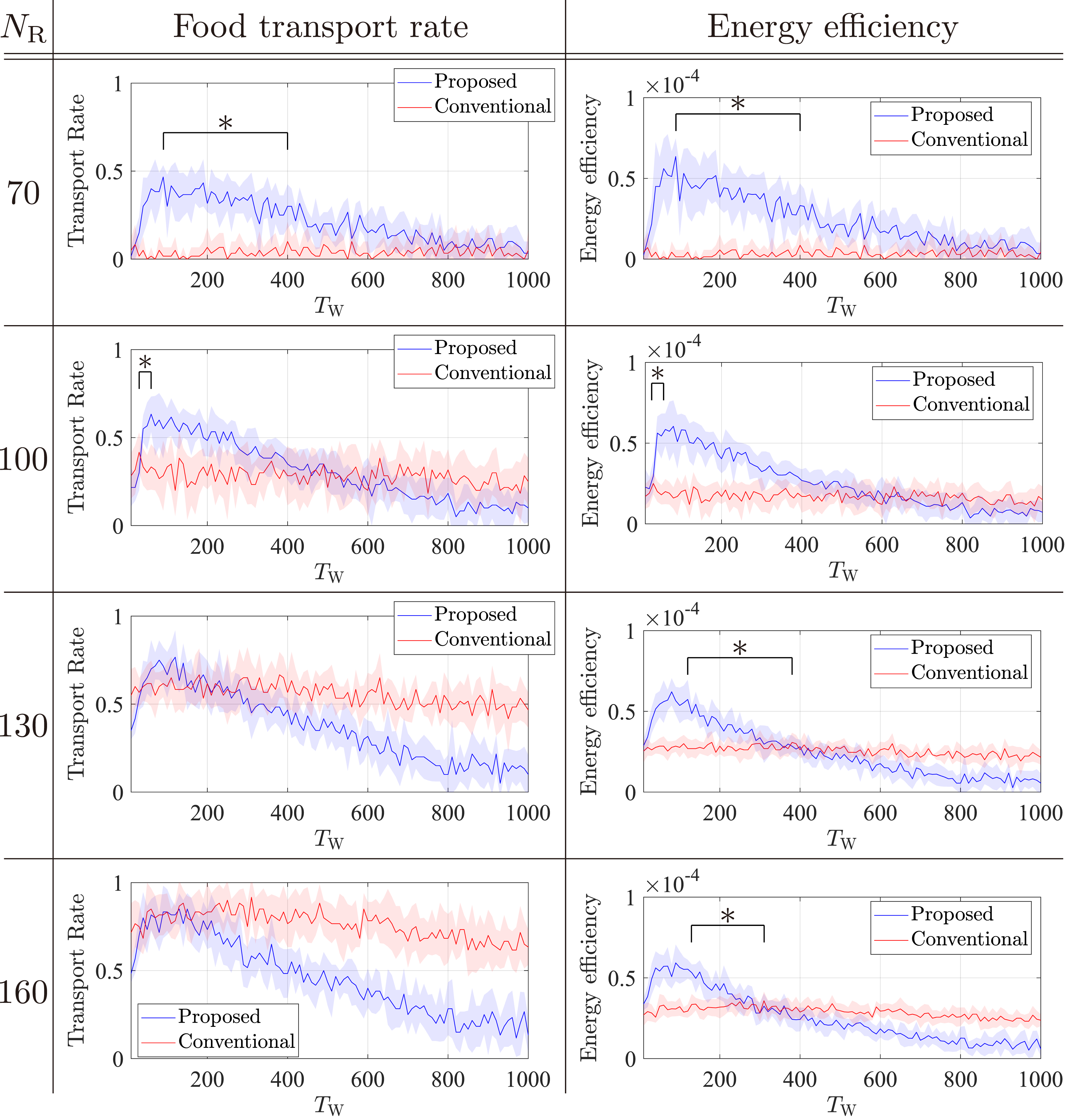

Next, we compared energy efficiency. The proposed model outperforms the conventional model in maximum energy efficiency for all population sizes for the same reasons described in Section 5.2.1.

5.3.2. Reasons for the performance differences

Next, we discuss the reasons for the performance differences caused by various population sizes. Figure 10 shows average task allocation rate for proposed and conventional models. From Figure 10 and discussions in Section 5.2.2, we can infer that the average density of robots that can start following in the proposed model is always larger than that in the conventional model.

Figure 10.

Average task allocation rates for proposed and conventional models with different T_W over 10 runs under N_F = 6 and various N_R.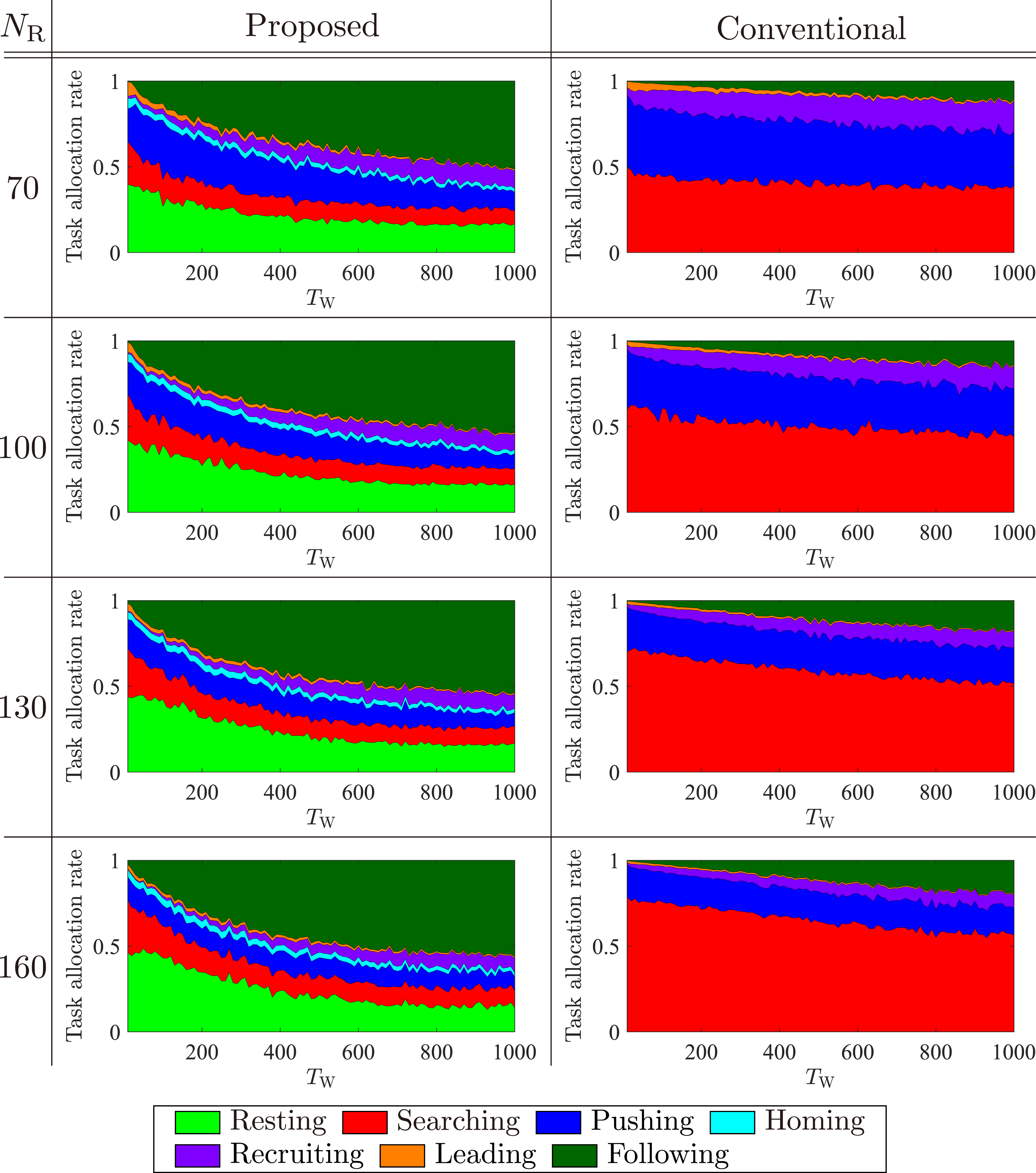

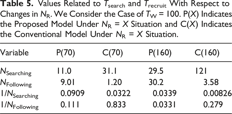
Table 5 summarizes N_Searching and N_Following of both models in the two cases of N_R, which are obtained by the results in Figure 10. From Table 5, 1/N_Following in the conventional model is 0.833 for N_R = 70 and 0.279 for N_R = 160. As a result, T_recruit in the conventional model dramatically decreases as N_R increases. By contrast, N_Searching in the proposed model dramatically increases as N_R increases. Hence, T_search in the proposed model dramatically decreases as N_R increases. Assuming that T_search is much larger than T_recruit, T_search is the main part of T_tot. By contrast, assuming that T_recruit is much larger than T_search, T_recruit is for the main part of T_tot. For the parameter settings of this study, T_recruit is the main part of T_tot. Thus, as N_R increases, the food transport rate in the conventional model dramatically increases (Figure 9). We can hence understand the reason why the small N_R environment is a situation in which the resting behavior dominates.

Table 5.

Values Related to T_search and T_recruit With Respect to Changes in N_R. We Consider the Case of T_W = 100. P(X) Indicates the Proposed Model Under N_R = X Situation and C(X) Indicates the Conventional Model Under N_R = X Situation.

Variable	P(70)	C(70)	P(160)	C(160)
N _Searching	11.0	31.1	29.5	121
N _Following	9.01	1.20	30.2	3.58
1/N_Searching	0.0909	0.0322	0.0339	0.00826
1/N_Following	0.111	0.833	0.0331	0.279

Next, we summarize the population-dependent differences. When the population is small, gathering a sufficient number of robots is difficult. In this scenario, the robots in the proposed model discover fewer food items, but most of these items are successfully transported to the nest owing to the effective recruitment. By contrast, the robots in the conventional model discover more food items, but only a few of them are transported to the nest because of the ineffective recruitment. Therefore, the time needed to gather a sufficient number of robots affects food transportation the most; thus, the proposed model outperforms the conventional model in food transport rate.

When the population is large, gathering a sufficient number of robots is easy. In this scenario, the robots in the proposed model discover fewer food items, which are successfully transported. By contrast, the robots in the conventional model also discover more food items, which are again successfully transported. Therefore, the time to discover a food item affects food transportation the most; thus, the conventional model outperforms the proposed model in food transport rate.

5.4. Summary of the performance of both models

We summarize relationship between N_R, N_F, and foraging performance. N_R was set to 70, 100, 130, 160, and for each N_R, N_F was set to 6, 8, 10, 12.

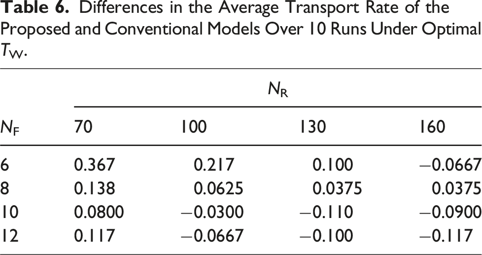
Table 6 and Table 7 show the quantitative differences in the performances of the proposed and conventional models for four types of N_R and N_F. The performance results of the conventional model subtracted from those of the proposed model are shown. The performances obtained using optimal T_W were compared. Figure 11 visually shows the results of Table 6 and Table 7. From the discussion in Sections 5.2 and 5.3, it is clear that the proposed model is dominant in small N_R environments and small N_F environments in terms of the transport rate (Figure 11(a)). Additionally, the proposed model always outperforms the conventional model in terms of energy efficiency regardless of N_R and N_F (Figure 11(b)).

Table 6.

Differences in the Average Transport Rate of the Proposed and Conventional Models Over 10 Runs Under Optimal T_W.

N _F	N _R
N _F	70	100	130	160
6	0.367	0.217	0.100	−0.0667
8	0.138	0.0625	0.0375	0.0375
10	0.0800	−0.0300	−0.110	−0.0900
12	0.117	−0.0667	−0.100	−0.117

Table 7.

Differences in the Average Energy Efficiency of the Proposed and Conventional Models Over 10 Runs Under Optimal T_W.

N _F	N _R
N _F	70	100	130	160
6	5.50×10⁻⁵	3.35×10⁻⁵	2.66×10⁻⁵	1.74×10⁻⁵
8	3.16×10⁻⁵	3.11×10⁻⁵	3.19×10⁻⁵	3.11×10⁻⁵
10	3.98×10⁻⁵	3.04×10⁻⁵	3.26×10⁻⁵	2.88×10⁻⁵
12	4.37×10⁻⁵	3.19×10⁻⁵	3.33×10⁻⁵	2.55×10⁻⁵

Figure 11.

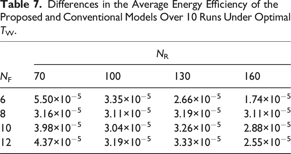
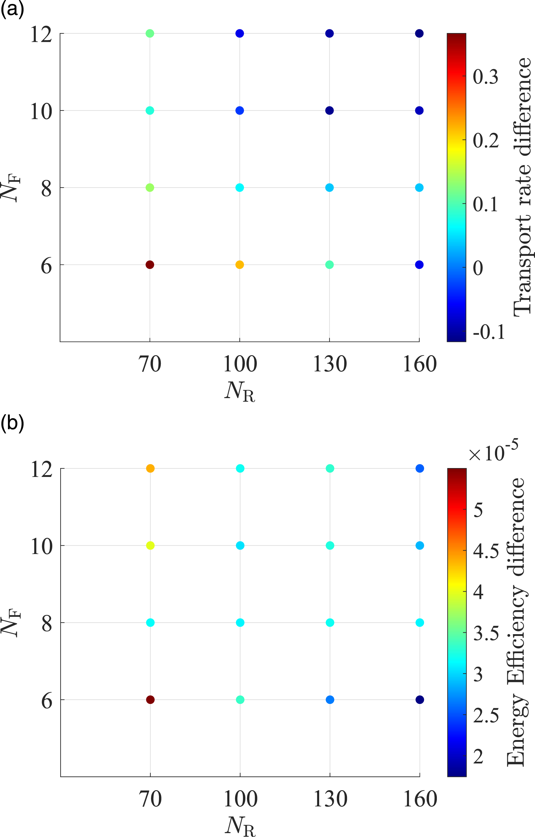
Differences in the average (a) transport rate and (b) energy efficiency of the proposed and conventional models over 10 runs under optimal T_W.

6. Conclusion and future extensions

In this study, we constructed a state-transition model for a swarm of robots for group foraging. In the proposed model, a state-transition model for solitary foraging including the resting behavior (Liu et al., 2007) and ant recruiting behavior for group foraging are combined.

Because of its resting behavior, the proposed model leads to more resting robots and fewer searching robots than the conventional state-transition model without the resting behavior. Moreover, the maximum search duration is limited, so exploration at distant sites is not sufficient. Therefore, the proposed model underperforms the conventional model in food item discovery. By contrast, because of the resting behavior, the nest functions as a gathering spot and therefore the robot density inside the nest is high. Therefore, recruiting robots can recruit many robots quickly inside the nest. In this way, the resting robots function as a potential labor pool. As a result, the proposed model outperforms the conventional model in gathering sufficient number of robots.

Regarding the evaluation of the transport rate, when each food item in the environment is light or there are many robots in the swarm, the proposed model underperforms the conventional model. This is because the time required to discover a food item is important in those situations. However, the proposed model, which includes the resting behavior, is dominant in environments where heavy food items are scattered and population in the swarm is small. This is because the time required to gather a sufficient number of robots is important in such situations. Regarding the evaluation of energy efficiency, the proposed model always outperforms the conventional model. This is because resting robots save energy when they are not needed; they are recruited and consume energy only when they are needed.

The well-known central-place foraging approach is defined as a set of foraging behaviors, that is, departure from a place, searching for food items at distant sites, and returning to the same place (Olsson et al., 2008). In central-place foraging, a return trip is necessary, and hence the search range is constrained. However, a central place provides benefits exceeding the constraint, for example, a safe resting place and frequent interaction between agents (Davidson et al., 2016). In this study, recruitment through frequent interaction between robots increased the speed of foraging, and hence it is consistent with the characteristics of central-place foraging.

For future extensions, we would like to introduce adaptive versions of the parameters T_R, T_S, T_P, and T_W that change in response to changes in N_R and N_F. Additionally, a real robot experiment will be a primary challenge.

Supplemental Material

Supplemental Material - Investigating dominant situation of resting behavior as a potential labor pool in robotic swarm for group foraging

Supplemental Material for Investigating dominant situation of resting behavior as a potential labor pool in robotic swarm for group foraging by Tomohiro Hayakawa, Toshiyuki Yasuda, and Fumitoshi Matsuno in Adaptive Behavior

Footnotes

Authors’ note

We have uploaded two videos showing whole simulation about Figures 5 and 6. Additionally, we have uploaded a figure showing the influence of changing m_total. All of the code used in this study has been uploaded to GitHub ().

Declaration of conflicting interests

The author(s) declared no potential conflicts of interest with respect to the research, authorship, and/or publication of this article.

Funding

The author(s) received no financial support for the research, authorship, and/or publication of this article.

ORCID iD

Tomohiro Hayakawa

Supplemental Material

Supplemental material for this article is available online.

About the Authors

Tomohiro Hayakawa received the B.E., M.E., and PhD degrees in mechanical engineering, in 2015, 2017, and 2020, respectively, from Kyoto University, Kyoto, Japan. From 2021 to 2023, he has been an assistant Professor with the Faculty of Engineering, University of Toyama. Since 2024, he has been an assistant professor with the Department of Mechanical Engineering, Faculty of Engineering, Shizuoka University. His research interests include multi-legged robot, swarm robotics, and reconfigurable modular robot.

Toshiyuki Yasuda received B.E., M.E., and PhD degrees in engineering in 2000, 2002, and 2006, respectively, from Kobe University, Japan. From 2006 to 2007, he was a research associate at Tsuyama National College of Technology. Before joining University of Toyama as an associate professor in 2017, he was an assistant professor at Hiroshima University for 10 years. Since 2023, he has been a professor with Faculty of Engineering, University of Toyama, Japan. His research areas cover artificial intelligence and autonomous agents. His current research interests include learning and evolutionary approaches to swarm robot systems.

Fumitoshi Matsuno received the Dr.Eng. degree in control engineering from Osaka University in 1986. The same year, he joined the Department of Control Engineering at Osaka University. From 2009 to 2023, he served as a Professor in the Department of Mechanical Engineering and Science at Kyoto University. Since 2023, he has held multiple roles: Professor in the Department of Electronics and Information Systems Engineering at Osaka Institute of Technology, Deputy Director of the Robotics Field at the Fukushima Institute for Research, Education, and Innovation (F-REI), and Professor Emeritus at Kyoto University. In addition, he is the Vice-President of the NPO International Rescue System Institute and served as the President of the Institute of Systems, Control, and Information Engineers and as Vice-President of the Robotics Society of Japan. His current research interests include robotics, swarm intelligence, control of distributed parameter and nonlinear systems, and disaster rescue support systems.

References

Barrientos

Colorado

Cerro

Martinez

Rossi

Sanz

Valente

(2011). Aerial remote sensing in agriculture: A practical approach to area coverage and path planning for fleets of mini aerial robots. Journal of Field Robotics, 28(5), 667–689. https://doi.org/10.1002/rob.20403

Bayindir

(2016). A review of swarm robotics tasks. Neurocomputing, 172(4), 292–321. https://doi.org/10.1016/j.neucom.2015.05.116

Berman

Lindsey

Sakar

M. S.

Kumar

Pratt

S. C.

(2011). Experimental study and modeling of group retrieval in ants as an approach to collective transport in swarm robotic systems. Proceedings of the IEEE, 99(9), 1470–1481. https://doi.org/10.1109/JPROC.2011.2111450

Bonabeau

Theraulaz

Deneubourg

J. L.

(1998). Fixed response thresholds and the regulation of division of labor in insect societies. Bulletin of Mathematical Biology, 60(4), 753–807. https://doi.org/10.1006/bulm.1998.0041

Brambilla

Ferrante

Birattari

Dorigo

(2013). Swarm robotics: A review from the swarm engineering perspective. Swarm Intelligence, 7(1), 1–41. https://doi.org/10.1007/s11721-012-0075-2

Brutschy

Pini

Pinciroli

Birattari

Dorigo

(2014). Self-organized task allocation to sequentially interdependent tasks in swarm robotics. Autonomous Agents and Multi-Agent Systems, 28(1), 101–125. https://doi.org/10.1007/s10458-012-9212-y

Castello

Yamamoto

Libera

F. D.

Liu

Winfield

A. F. T.

Nakamura

Ishiguro

(2016). Adaptive foraging for simulated and real robotic swarms: The dynamical response threshold approach. Swarm Intelligence, 10(1), 1–31. https://doi.org/10.1007/s11721-015-0117-7

Castello

Yamamoto

Nakamura

Ishiguro

(2013). Task allocation for a robotic swarm based on an adaptive response threshold model. 13th International Conference on Control, Automation and Systems (ICCAS 2013), 259–266. https://doi.org/10.1109/ICCAS.2013.6703905

Charbonneau

Dornhaus

(2015). When doing nothing is something. how task allocation strategies compromise between flexibility, efficiency, and inactive agents. Journal of Bioeconomics, 17(3), 217–242. https://doi.org/10.1007/s10818-015-9205-4

10.

Charbonneau

Sasaki

Dornhaus

(2017). Who needs ‘lazy’ workers? Inactive workers act as a ‘reserve’ labor force replacing active workers, but inactive workers are not replaced when they are removed. PLoS One, 12(9), Article e0184074. https://doi.org/10.1371/journal.pone.0184074

11.

Chen

Gauci

Kolling

Gros

(2015). Occlusion-based cooperative transport with a swarm of miniature mobile robots. IEEE Transactions on Robotics, 31(2), 307–321. https://doi.org/10.1109/TRO.2015.2400731

12.

Daly-Schveitzer

Beugnon

Lachaud

J. P.

(2007). Prey weight and overwhelming difficulty impact the choice of retrieval strategy in the neotropical ant gnamptogenys sulcata (f. smith). Insectes Sociaux, 54(4), 319–328. https://doi.org/10.1007/s00040-007-0949-2

13.

Davidson

J. D.

Arauco-Aliaga

R. P.

Crow

Gordon

D. M.

Goldman

M. S.

(2016). Effect of interactions between harvester ants on forager decisions. Frontiers in Ecology and Evolution, 4(1), 115–117. https://doi.org/10.3389/fevo.2016.00115

14.

Digani

Sabattini

Secchi

Fantuzzi

(2013). Towards decentralized coordination of multi robot systems in industrial environments: A hierarchical traffic control strategy. In 2013 IEEE 9th international conference on intelligent computer communication and processing (ICCP) (pp. 209–215). IEEE. https://doi.org/10.1109/ICCP.2013.6646110

15.

Farivarnejad

Wilson

Berman

(2016). Decentralized sliding mode control for autonomous collective transport by multi-robot systems. In 2016 IEEE 55th conference on decision and control (pp. 1826–1833). CDC. https://doi.org/10.1109/CDC.2016.7798530

16.

Feinerman

Pinkoviezky

Gelblum

Fonio

Gov

N. S.

(2018). The physics of cooperative transport in groups of ants. Nature Physics, 14(7), 683–693. https://doi.org/10.1038/s41567-018-0107-y

17.

Ferrante

Turgut

A. E.

Duéñez-Guzmán

Dorigo

Wenseleers

(2015). Evolution of self-organized task specialization in robot swarms. PLoS Computational Biology, 11(8), Article e1004321. https://doi.org/10.1371/journal.pcbi.1004273

18.

Fujisawa

Dobata

Sugawara

Matsuno

(2014). Designing pheromone communication in swarm robotics: Group foraging behavior mediated by chemical substance. Swarm Intelligence, 8(3), 227–246. https://doi.org/10.1007/s11721-014-0097-z

19.

Gross

Bonani

Mondada

Dorigo

(2006). Autonomous self-assembly in swarm-bots. IEEE Transactions on Robotics, 22(6), 1115–1130. https://doi.org/10.1109/TRO.2006.882919

20.

Hamann

(2013). Towards swarm calculus: Urn models of collective decisions and universal properties of swarm performance. Swarm Intelligence, 7(2-3), 145–172. https://doi.org/10.1007/s11721-013-0080-0

21.

Hasegawa

Ishii

Tada

Kobayashi

Yoshimura

(2016). Lazy workers are necessary for long-term sustainability in insect societies. Scientific Reports, 6(1), Article 20846. https://doi.org/10.1038/srep20846

22.

Hayakawa

Dobata

Matsuno

(2020). Behavioral responses to colony-level properties affect disturbance resistance of red harvester ant colonies. Journal of Theoretical Biology, 492(1), Article 110186. https://doi.org/10.1016/j.jtbi.2020.110186

23.

Hunt

E. R.

Jones

Hauert

(2019). Testing the limits of pheromone stigmergy in high-density robot swarms. Royal Society Open Science, 6(11), Article 190225. https://doi.org/10.1098/rsos.190225

24.

Ijspeert

A. J.

Martinoli

Billard

Gambardella

L. M.

(2001). Collaboration through the exploitation of local interactions in autonomous collective robotics: The stick pulling experiment. Autonomous Robots, 11(2), 149–171. https://doi.org/10.1023/A:1011227210047

25.

Jin

Liang

Han

Ohkura

(2020). Generating collective foraging behavior for robotic swarm using deep reinforcement learning. Artificial Life and Robotics, 25(4), 588–595. https://doi.org/10.1007/s10015-020-00642-2

26.

Jurt

Milner

Sooriyabandara

Hauert

(2022). Collective transport of arbitrarily shaped objects using robot swarms. Artificial Life and Robotics, 27(2), 365–372. https://doi.org/10.1007/s10015-022-00730-5

27.

Kantor

Singh

Peterson

Rus

Das

Kumar

Pereira

Spletzer

(2006). Distributed search and rescue with robot and sensor teams. Field and Service Robotics, 24(1), 529–538.

28.

Krieger

M. J. B.

Billeter

J. B.

(2000). The call of duty: Self-organised task allocation in a population of up to twelve mobile robots. Robotics and Autonomous Systems, 30(1-2), 65–84. https://doi.org/10.1016/s0921-8890(99)00065-2

29.

Labella

T. H.

Dorigo

Deneubourg

J. L.

(2006). Division of labor in a group of robots inspired by ants’ foraging behavior. ACM Transactions on Autonomous and Adaptive Systems, 1(1), 4–25. https://doi.org/10.1145/1152934.1152936

30.

Lee

Vaughan

Kim

(2020). Task allocation into a foraging task with a series of subtasks in swarm robotic system. IEEE Access, 8(1), 107549–107561. https://doi.org/10.1109/ACCESS.2020.2999538

31.

Liu

Winfield

A. F. T.

(2010). Modeling and optimization of adaptive foraging in swarm robotic systems. The International Journal of Robotics Research, 29(14), 1743–1760. https://doi.org/10.1177/0278364910375139

32.

Liu

Winfield

A. F. T.

Chen

Dou

(2007). Towards energy optimization: Emergent task allocation in a swarm of foraging robots. Adaptive Behavior, 15(3), 289–305. https://doi.org/10.1177/1059712307082088

33.

McCreery

H. F.

Breed

M. D.

(2014). Cooperative transport in ants: A review of proximate mechanisms. Insectes Sociaux, 61(2), 99–110. https://doi.org/10.1007/s00040-013-0333-3

34.

Mondada

Gambardella

Floreano

Nolfi

Deneubourg

Dorigo

(2005). The cooperation of swarm-bots: Physical interactions in collective robotics. IEEE Robotics and Automation Magazine, 12(2), 21–28. https://doi.org/10.1109/MRA.2005.1458313

35.

Nouyan

Gross

Bonani

Mondada

Dorigo

(2009). Teamwork in self-organized robot colonies. IEEE Transactions on Evolutionary Computation, 13(4), 695–711. https://doi.org/10.1109/TEVC.2008.2011746

36.

Olsson

Brown

J. S.

Helf

K. L.

(2008). A guide to central place effects in foraging. Theoretical Population Biology, 74(1), 22–33. https://doi.org/10.1016/j.tpb.2008.04.005

37.

Pini

Brutschy

Frison

Roli

Dorigo

Birattari

(2011). Task partitioning in swarms of robots: An adaptive method for strategy selection. Swarm Intelligence, 5(3-4), 283–304. https://doi.org/10.1007/s11721-011-0060-1

38.

Pini

Gagliolo

Brutschy

Dorigo

Birattari

(2013). Task partitioning in a robot swarm: A study on the effect of communication. Swarm Intelligence, 7(2-3), 173–199. https://doi.org/10.1007/s11721-013-0078-7

39.

Radeva

Dornhaus

Lynch

Nagpal

H. H.

(2017). Costs of task allocation with local feedback: Effects of colony size and extra workers in social insects and other multi-agent systems. PLoS Computational Biology, 13(12), e1005904–e1005929. https://doi.org/10.1371/journal.pcbi.1005904

40.

Reynolds

C. W.

(1987). Flocks, herds and schools: A distributed behavioral model. SIGGRAPH Comput. Graph, 21(4), 25–34. https://doi.org/10.1145/37402.37406

41.

Schmickl

Karsai

(2014). Sting, carry and stock: How corpse availability can regulate de-centralized task allocation in a ponerine ant colony. PLoS One, 9(12), Article e114611. https://doi.org/10.1371/journal.pone.0114611

42.

Wang

Schwager

(2016). Kinematic multi-robot manipulation with no communication using force feedback. In 2016 IEEE international conference on robotics and automation (ICRA) (pp. 427–432). IEEE. https://doi.org/10.1109/ICRA.2016.7487163

43.

Wilson

E. O.

(1984). The relation between caste ratios and division of labor in the ant genus Pheidole (Hymenoptera: Formicidae). Behavioral Ecology and Sociobiology, 16(1), 89–98. https://doi.org/10.1007/BF00293108

44.

Wilson

Buffin

Pratt

S. C.

Berman

(2018). Multi-robot replication of ant collective towing behaviours. Royal Society Open Science, 5(10), Article 180409. https://doi.org/10.1098/rsos.180409

45.

Yang

Zhou

Tian

(2009) Swarm robots task allocation based on response threshold model. In: 2009 4th international conference on autonomous robots and agents (pp. 171–176). IEEE. https://doi.org/10.1109/ICARA.2000.4803959

46.

Yoshimoto

Endo

Maeda

Matsuno

(2018). Decentralized navigation method for a robotic swarm with nonhomogeneous abilities. Autonomous Robots, 42(8), 1583–1599. https://doi.org/10.1007/s10514-018-9774-x

47.

Yasuda

Ohkura

Matsumura

Goka

(2013). Cooperative transport by a swarm robotic system based on cma-neuroes approach. Journal of Advanced Computational Intelligence and Intelligent Informatics, 17(6), 932–942. https://doi.org/10.20965/jaciii.2013.p0932

48.

Zahugi

E. M. H.

Shabani

A. M.

Prasad

T. V.

(2012). Libot: Design of a low cost mobile robot for outdoor swarm robotics. In 2012 IEEE international conference on cyber Technology in automation, control, and intelligent systems (CYBER) (pp. 342–347). IEEE. https://doi.org/10.1109/CYBER.2012.6392577

Supplementary Material

Please find the following supplemental material available below.

For Open Access articles published under a Creative Commons License, all supplemental material carries the same license as the article it is associated with.

For non-Open Access articles published, all supplemental material carries a non-exclusive license, and permission requests for re-use of supplemental material or any part of supplemental material shall be sent directly to the copyright owner as specified in the copyright notice associated with the article.

0.00 MB

0.25 MB