Deep learning models for predictive maintenance in Industry 4.0: An analysis

Abstract

This paper focuses on exploring the use cases and practical applicability of deep learning in Industry 4.0 by studying on a water pump time series dataset with 5 models namely LSTM, CNN-LSTM, GAF-CNN, BiLSTM and Time-Series Transformer. The unplanned downtime due to sudden equipment failure costs the industry huge losses every year. The proposed methodology based on deep learning architectures uses sensor readings and leads to meaningful predictions for cost-cutting and time saving. The study evaluates and compares these models in terms of fine-grained architecture-level components and prediction accuracy. The results demonstrated that the transformer based time series hybrid model is more accurate in prediction with balanced performance and strong interpretability than other models.

Keywords

deep learning LSTM CNN-LSTM GAF-CNN BiLSTM time-series

Introduction

Mechanical asset failure can lead to downtime, costly repairs, and potential safety hazards in industries. Traditionally, maintenance strategies were based on scheduled approaches that are often inefficient in unexpected breakdowns (Hakami, 2024). As industries continue to embrace the principles of Industry 4.0, there is growing demand for intelligent automated solutions that can anticipate failures and optimize the maintenance process driven by the economic necessity to mitigate unplanned downtime (Achouch et al., 2022).

According to the Aberdeen Group (2016), global manufacturing incurs approximately US $1 trillion in annual losses due to such failures. In the specific context of industrial pumping systems, the Hydraulic Institute and Europump estimate that maintenance and downtime account for roughly 25% of the total lifecycle expenditure—significantly higher than the initial purchase cost 10% (Hydraulic Institute and Europump, 2001). Therefore, the deep learning models analyzed in this study are not merely classifiers but critical enablers of the Industry 4.0 ‘Smart Factory'. By predicting failures before they occur, these architectures directly address the 25% cost burden, facilitating the shift from reactive repairs to autonomous, predictive lifecycle management (Lee et al.,, 2013).

Deep learning has shown promise in this domain due to its ability to extract temporal and spatial features from large, multivariate datasets. Among various deep learning architectures, Long Short-Term memory (LSTM) networks, BiLSTM, Convolutional Neural network combined with LSTM (CNN-LSTM), Gramian Angular Field - Convolutional Neural Networks (GAF-CNN), Transformer based networks have gained considerable attention. LSTM networks are effective in modeling sequential dependencies and capturing temporal patterns in time - series data (Hochreiter and Schmidhuber, 1997). BiLSTM network works in both forward and backward direction to capture recent and past data for accurate prediction (Schuster and Paliwal, 1997). CNN-LSTM hybrid model combines strengths of CNNs local feature extraction with LSTMs capability to model long term temporal dependencies making it well suited for complex degradation processes (Ordonez and Roggen, 2016). GAF-CNN approaches transform time-series data into two dimensional images using Gramian Angular Fields, allowing CNN to learn discriminative spatial features from encoded time-series pattern (Zhang, 2025). Transformer based time series model is beneficial with ample amount of data for prediction.

Despite of their promising performance, these architectures also present challenges related to data requirements and pre-processing, interpretability, model complexity and deployment in real time applications. Specifically, the existing approaches present the following challenges which must be addressed. LSTM model is effective in identifying temporal dependencies, often struggles with very long sequential data it can be computationally intensive. BiLSTM model improves these by spanning in both the directions simultaneously but leads to high computational cost and memory requirements which becomes unsuitable for real time applications. CNN-LSTM combines sequential modeling and local feature extraction, but if there persists flaw in designing convolutional layer, then performance of model may degrade. These trade-offs underscores importance of comparing different data models to identify the most suitable model for time series data.

Our contributions

Besides comparing deep learning models for accuracy, this work is distinguished by evaluating its operational and practical feasibility of the architecture for edge computing and industrial digital twin.

(1) Baseline for Edge Deployment: Assessing the trade-offs in storage and computational cost to identify models suitable for embedded devices. This facilitates on-spot processing, eliminating the need to export sensitive sensor data to the cloud and thereby preserving industrial data using embedded systems.

(2) Enablement of Digital Twin: Analyzing model interpretability and latency to enable ’policy twins’— digital counterparts that allow operators to answer ’what-if’ maintenance questions (e.g., simulating deferred maintenance scenarios) before implementation.

(3) Trade-off Analysis: Systematically categorize the strengths and weaknesses of LSTM, CNN-LSTM, GAF-CNN, and Transformers to guide the selection of architectures that balance fault detection with the resource constraints of IoT infrastructure.

Paper organization

The remainder of this paper is organized as follows:

• Section II reviews various deep learning models for predictive maintenance and identifies research gaps.

• Section III details methodology which includes data description, data preprocessing, class distribution, model architectures and their workflow. It also mentions the Implementation hyperparameters selection and evaluation metrics.

• Section IV presents experimental result and comparative performance analysis based on accuracy, F1 score, precision, recall etc. It highlights the discussion based on the comparative analysis.

• Finally, Section V represents conclusion obtained and future directions of the study.

Related works

Deep learning models have become the cornerstone of modern predictive maintenance with powerful tools for learning spatial patterns, temporal dependencies and image encoded time-series in context of Industry 4.0. In particular LSTM, BiLSTM, CNN-LSTM, GAF-CNN, Transformer based architectures are leading frameworks to predict Remaining Useful Life (RUL) and fault detection. Various recent approaches have been proposed to enhance predictive maintenance capabilities, each comes with specific limitations regarding data requirements, scalability and interpretability.

Ho et al. (2025) employed reinforcement learning for planning dynamic path of automated guided vehicles in smart logistics and operations, improving efficiency in automated manufacturing system. Drakaki et al. (2022) provided a comprehensive survey on deep learning and machine learning methods towards Industry 4.0 for predictive maintenance in induction motors highlighting techniques that improves operational efficiency and reduce downtime. Kotsiopoulos et al. (2021) explored the integration of machine learning and deep learning in smart manufacturing systems to optimize production process and resource management. Integration of Remaining Useful life (RUL) of machinery into decision making becomes a critical task in predictive maintenance. Wang et al., (2025a) demonstrated how predictive maintenance strategy can be optimized by combining RUL predictions. Similarly, Wang et al., (2025b) proposed novel formulation and metaheuristic algorithm mainly for aircraft engines illustrating RUL-driven optimization in high-stake engineering contexts.

Liu and Xu (2021) introduced LSTM, to predict RUL of roller bearings by capturing vibration signals. They demonstrate superior performance over LSTM based datasets. The methodology used here is pure sequenced LSTM, they often struggle with noisy and multivariate data sets. Yang and Peng (2022) proposed the LSTM framework with Monte Carlo Dropout and nonparametric kernel density and estimation of both RUL and prediction uncertainty and lacks built-in data interpretability. Hochreiter and Schmidhuber (1997) introduced LSTM networks providing base for handling sequential data effectively. Their work limelights the capability of LSTM to capture long term dependencies, crucial for time-series applications.

Schuster and Paliwal (1997); Isnain et al. (2020) presented bidirectional Recurrent Neural Networks spanning in both the direction simultaneously for fault prediction based on past and future states. This approach is better then simple RNN model but less suitable for real-time systems due to high computational cost then other models.

Khorram et al. (2021) presented a Convolutional Recurrent Neural Network (CRNN) that intakes raw accelerometer signals, applies 1D convolutions to extract local temporal features and feeds to LSTM layers for fault detection. This method outperforms hand-crafted feature methods on two benchmark vibration datasets without any preprocessing. Kiangala and Wang (2020) used CNN with time series imaging for predictive maintenance of conveyor motors, identifying research gap in LSTM sequential data processing.

Methodology

We analyze five deep learning models, i.e., LSTM model, BiLSTM model, CNN-LSTM hybrid model, GAF-CNN model and Transformer based model one after another to come up with efficient suitable technique for predictive maintenance of mechanical assets.

Dataset description

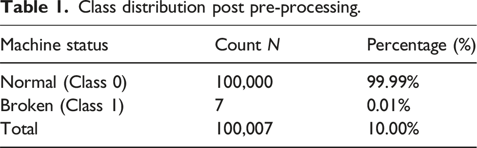
The dataset used in this study is obtained from the open-source Pump Sensor Data repository available on Kaggle (Phantawee, 2018). The dataset contains multivariate time-series sensor readings collected from an industrial pump system monitored continuously over operational cycles.

Table 1.

Class distribution post pre-processing.

Machine status	Count N	Percentage (%)
Normal (Class 0)	100,000	99.99%
Broken (Class 1)	7	0.01%
Total	100,007	10.00%

It is utilized to model the relationship between multivariate sensor trends and machine failure events. The predictive goal is to classify machine status at any given timestamp and forecast potential breakdowns before they occur, enabling timely maintenance intervention and reduced operational downtime and costs associated with it. The dataset contains 220320 time-stamped observations recorded at one-minute intervals. Each row corresponds to:

(timestamp, {sensor}_{00}, {sensor}_{01}, \dots, {sensor}_{51}, machine_status)

Data preprocessing and class distribution

The dataset comprises of sensor readings recorded at one-minute interval across 52 sensor channels. Raw data passes through several preprocessing stages including label refining, handling missing values, class balancing and feature preservation to ensure suitability for predictive modeling. Firstly, the data sets which are not suitable for binary classification are labeled as RECOVERING state. Data from sensors which are under RECOVERING state, nil or undefined are dropped to preserve integrity of time series pattern. Nearly 100,000 records are downsampled to reduce computational complexity, making them model-suitable. Following pre processing stages the class distribution of dataset is given in Table 1.

Model architecture and workflow

LSTM (Long short term memory)

LSTM model learns sequential data and avoids vanishing gradient issues using gates. The architecture of LSTM can be visualized as a series of repeating blocks. It includes:

• Input Layer: This layer ingests current input at each timestamp in sequence.

• LSTM Layers: The model comprises two stacked LSTM layers each containing hidden units. To reduce risk, dropout layers with dropout rate of 0.2 are inserted after each LSTM layer to prevent overfitting of data.

• Dense layers: Fully connected layer with sigmoid activation function to produce binary prediction.

As shown in Figure 1 the workflow of LSTM model begins with ingesting the raw data and performing initial cleansing i.e to drop corrupt entries. Cleaned data is then segmented into fixed length sequence and labeled after 10 consecutive spans, resulting into an input array of required format.

I n p u t s h a p e = (s a m p l e s, t i m e s t e p s, f e a t u r e s)

Figure 1.

LSTM Data flow.

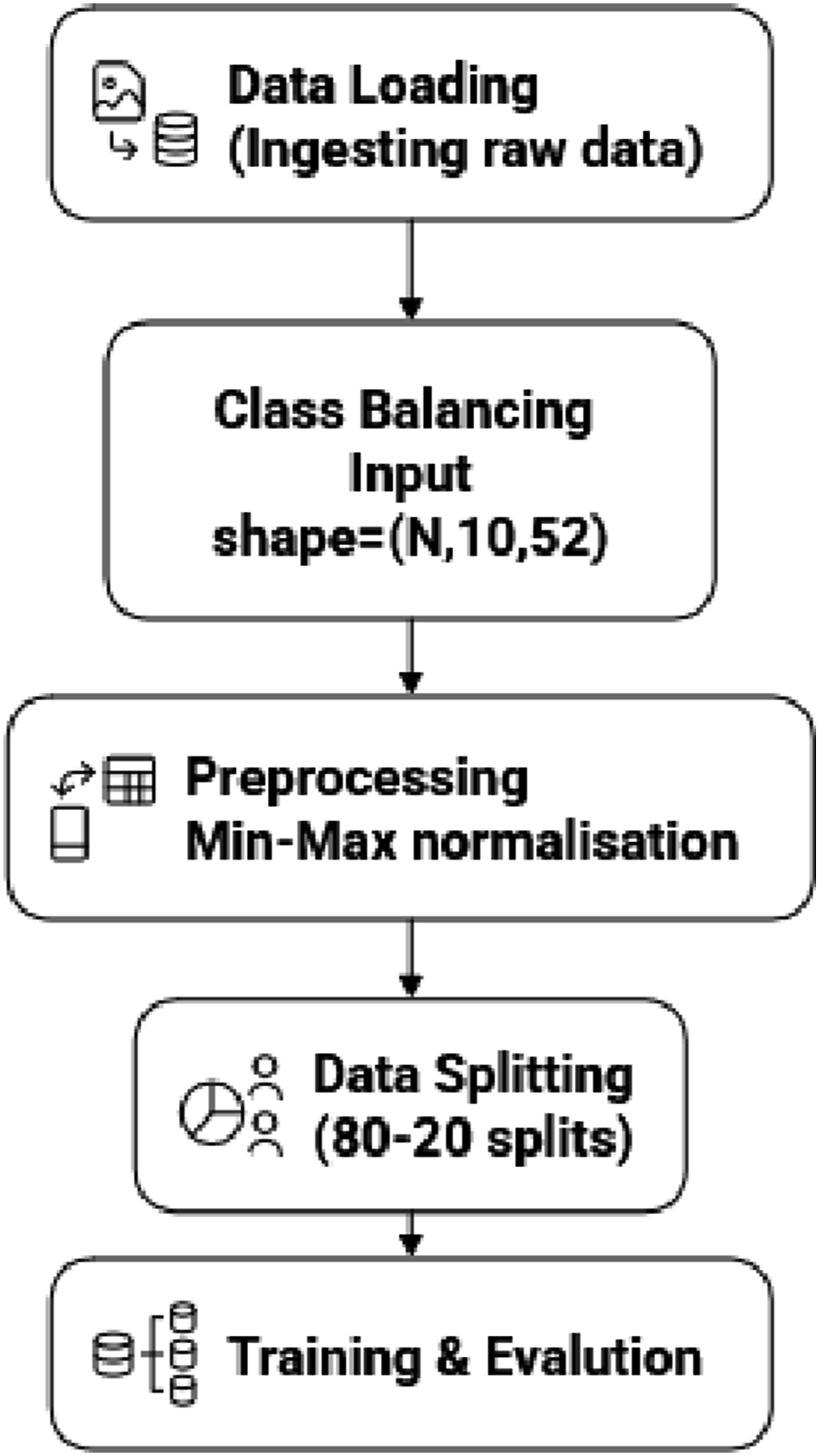
Data is then pre-processed using MinMax normalisation, readings are scaled to the range [0, 1]. Followed by preprocessing data is chronologically splited (Time based) into 80–20 splits to preserve temporal sequence of data and to prevent data leakage. 20% data from data split is fed for validation to enable early stopping and overfitting of data. 80% data from split is sent future for evaluation.

BiLSTM (Bidirectional long short term memory)

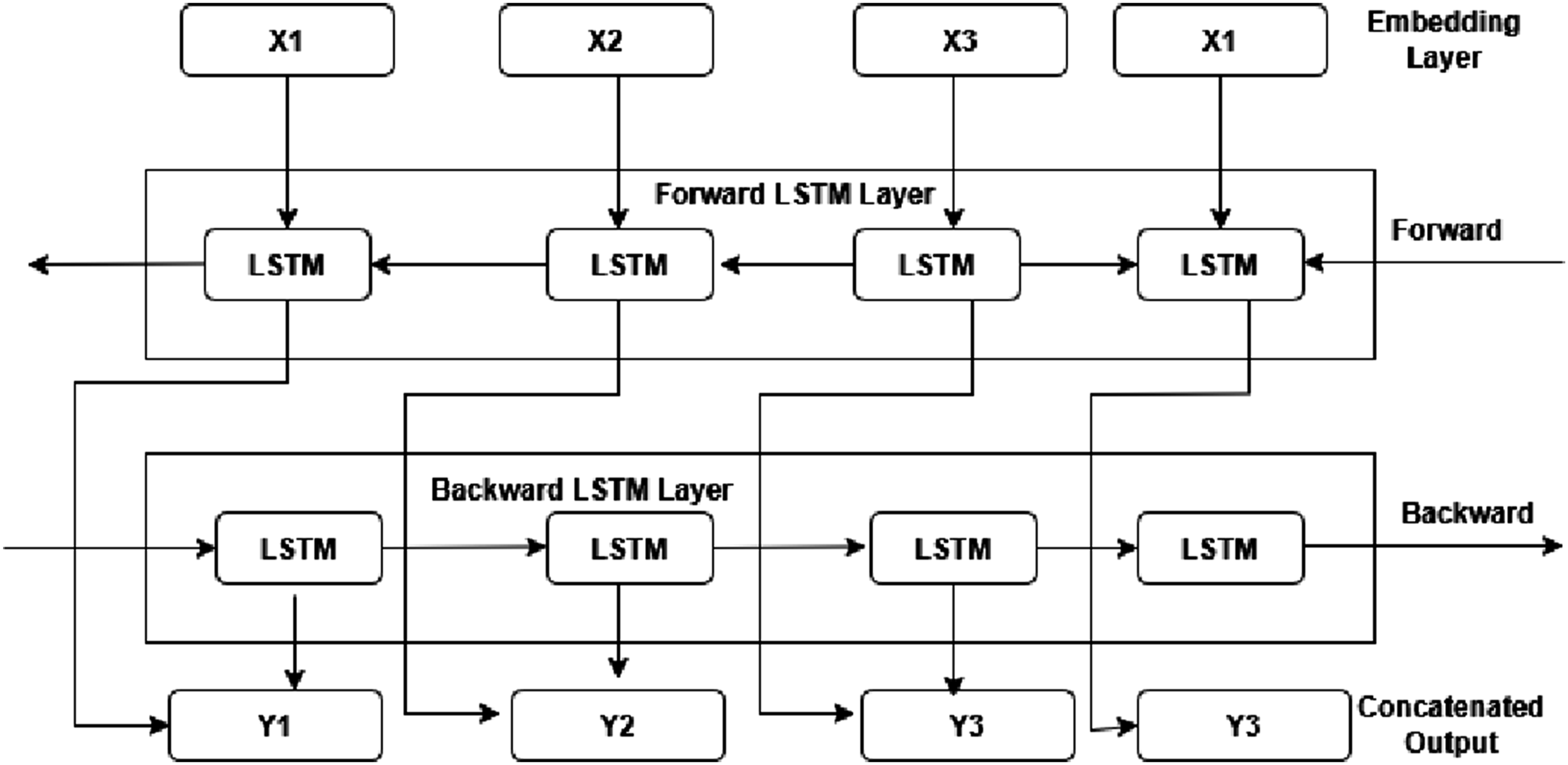
BiLSTM model is extended version of LSTM network, it processes data simultaneously in both forward and backward direction to avail data from past and future for accurate predictions. As shown in Figure 2 it includes two different forward and backward layer running in parallel connected to same output layer.

• Forward LSTM Layer: This layer processes the input sequence from beginning to end. At each time stamp it computes a hidden state having past information.

• Backward LSTM Layer: This layer processes the forward layers inputs sequence in reverse direction. At each time stamp it computes a hidden state having access to future information.

• Output Layer: Hidden state of both forward and backward layer is concatenated to produce final output in terms of past and future data.

Figure 2.

BiLSTM model.

As shown in Figure 3 the workflow of BiLSTM model begins with ingesting the raw data and performimg initial cleansing i.e to drop corrupt entries. Cleaned data is then segmented into fixed length sequence and labeled after 10 consecutive spans, resulting into an input array of required format.

I n p u t s h a p e = (s a m p l e s, t i m e s t e p s, f e a t u r e s)

Figure 3.

BiLSTM model data flow.

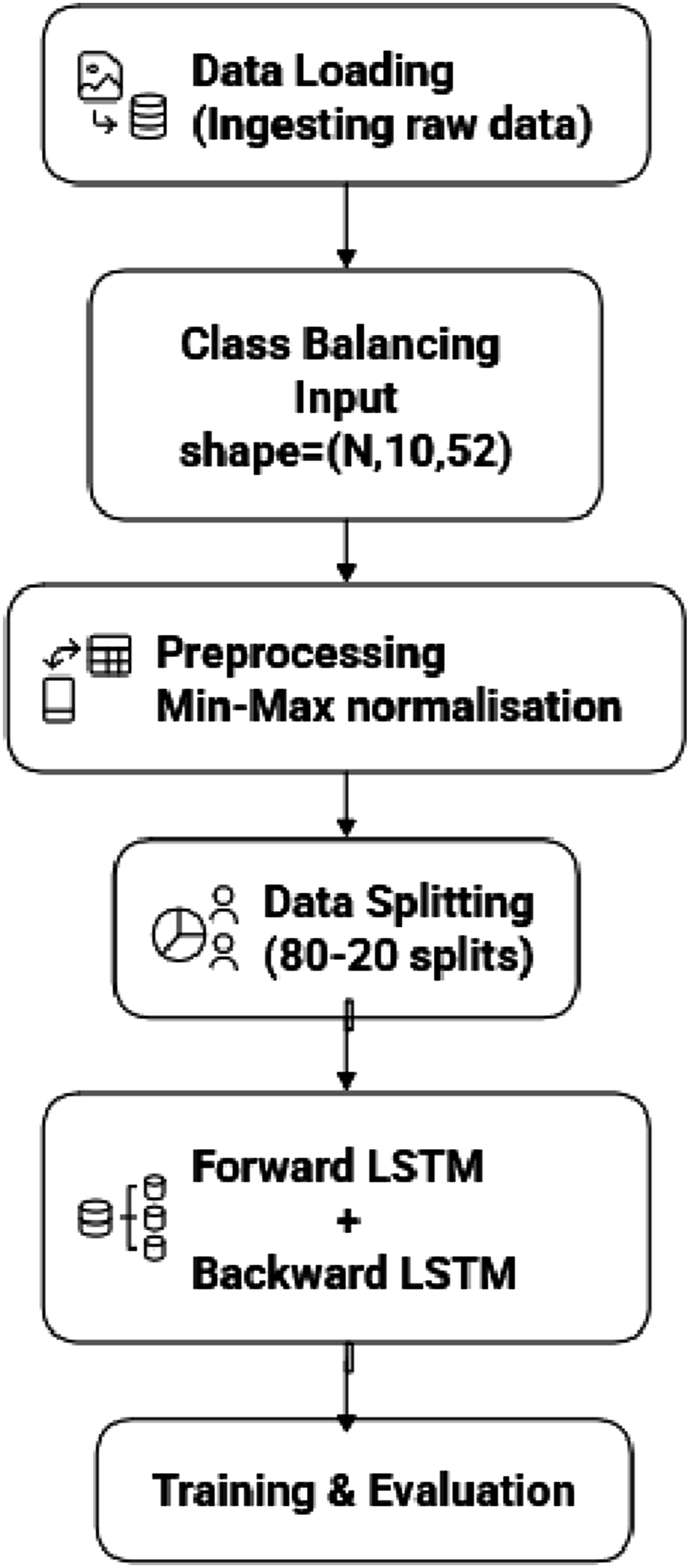
Data is then pre-processed using MinMax normalisation, readings ae scaled to the range [0, 1]. Followed by preprocessing data is chronologically splited (Time based) into 80–20 splits to preserve temporal sequence of data and to prevent data leakage. 20% data from data split is fed for validation to enable early stopping and overfitting of data. 80% split is sent to forward and backward LSTM layers which runs simultaneously. The output from both the layers is concatenated in the output layer and sent for evaluation.

LSTM-CNN hybrid model

Hybrid CNN-LSTM architecture combines the local feature-learning power of convolution networks with the temporal-dependency modeling recurrent units. As shown in Figure 4 hybrid model consists of:

• CNN Layers: Consists of one or two one dimensional convolutional layers and Max pooling layers for detecting recurring patterns and reducing sequence length.

• LSTM Layer: Refines data for suitable classification.

• Dense Layers: Fully connected layer for classification and regression of data.

Figure 4.

CNN-LSTM hybrid model.

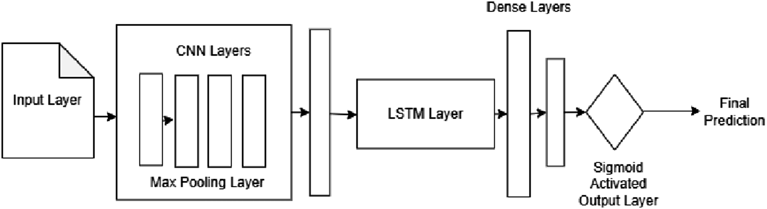
Workflow of CNN-LSTM model begins with ingesting the raw data and performimg initial cleansing i.e to drop corrupt entries. Cleaned data is then segmented into fixed length sequence and labeled after 10 consecutive spans, resulting into an input array of required format.

I n p u t s h a p e = (s a m p l e s, t i m e s t e p s, f e a t u r e s)

Data is then pre-processed using MinMax normalisation, readings ae scaled to the range [0, 1]. Followed by preprocessing data is chronologically splited (Time based) into 80–20 splits to preserve temporal sequence of data and to prevent data leakage and fed to CNN layers, here they are assembled into pooling blocks followed by stacked LSTM layers, dropout and dense classification head. Now the data set is optimised using Adam optimiser with early stopping based on validation loss.

Figure 5.

GAF-CNN model.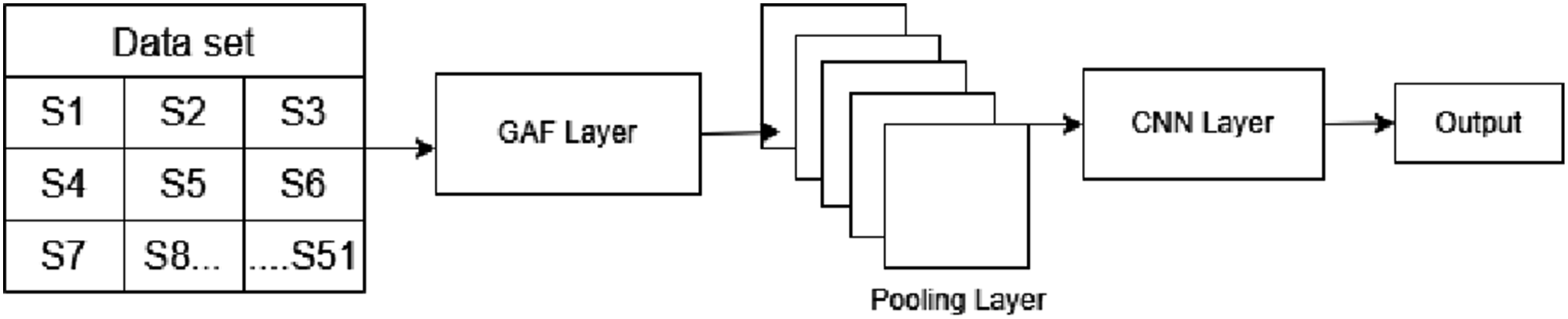

GAF-CNN model

As shown in Figure 5 GAF-CNN model consists of five stages:

• GAF Layer: Encodes 1D time series data to 2D matrix (image).

• Convolutional Layer: Filters are applied to input image to extract local features, followed by Rectified Linear Unit (ReLU) activation function for non-linearity.

• Pooling Layer: Reduces spatial dimensions and flattens data in one dimension undergoing many pooling stages.

• Fully Connected Layer: Learns higher-level representation and performs classification or regression task based on extracted features.

As shown in Figure 6 workflow of GAF-CNN model begins with ingesting the raw data and performing initial cleansing i.e to drop corrupt entries. Cleaned data is then reduced dimensionally using principal component analysis (PCA) to collapse 52- channel sensor data into a single time-series per sample

I n p u t s h a p e = (n_s a m p l e s, t i m e s t e p s, 1)

Figure 6.

GAF- CNN model data flow.

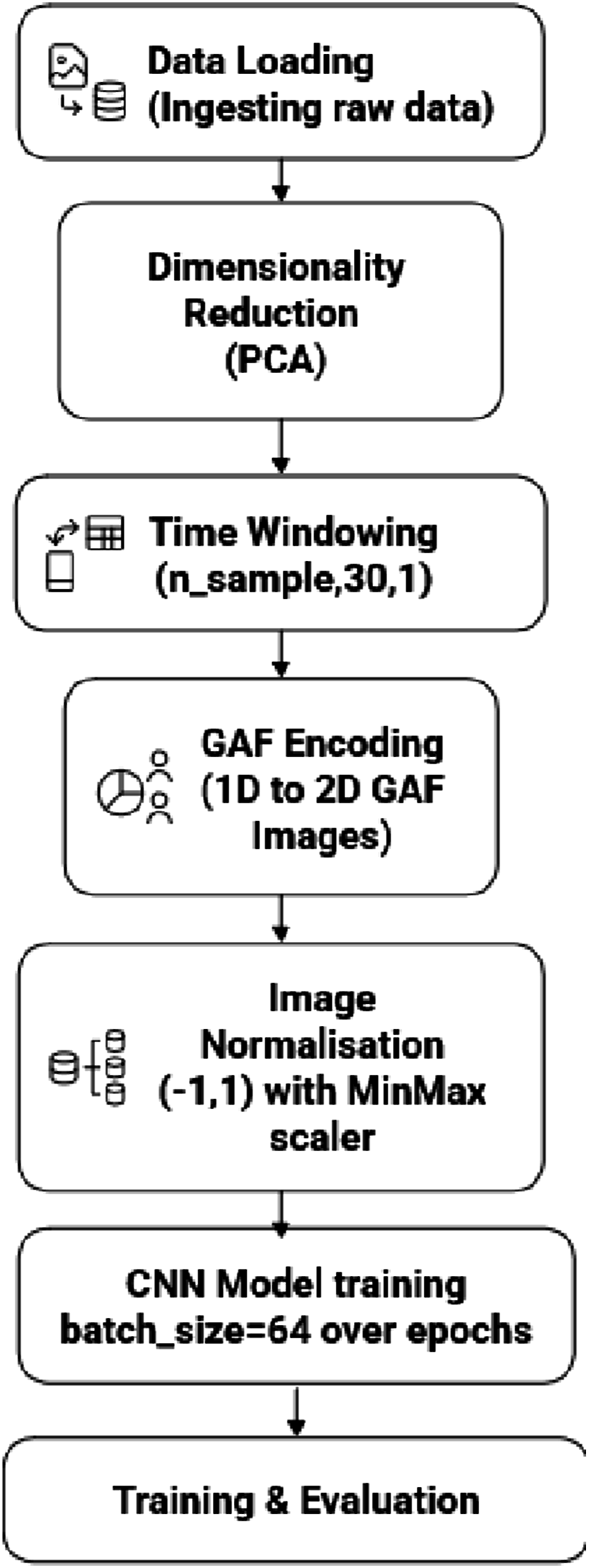
Overlapping window of length 30 is slid over each time series. Each 1D window is transformed into 2D GAF images using summation method. The images are normalized to [−1, 1] with MinMax scaler to stabilize CNN training. Data is then flatten in CNN layers and trained in batch size of 64 over several epochs and evaluated.

Time Series Transformer model

The Time Series Transformer model employs a self-attention mechanism to learn temporal dependencies directly from multivariate sensor data, without relying on recurrent computations. Unlike LSTM-based models that process inputs sequentially, the Transformer attends to all time steps in parallel, allowing it to effectively capture both short- and long-range temporal relationships.

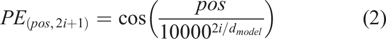
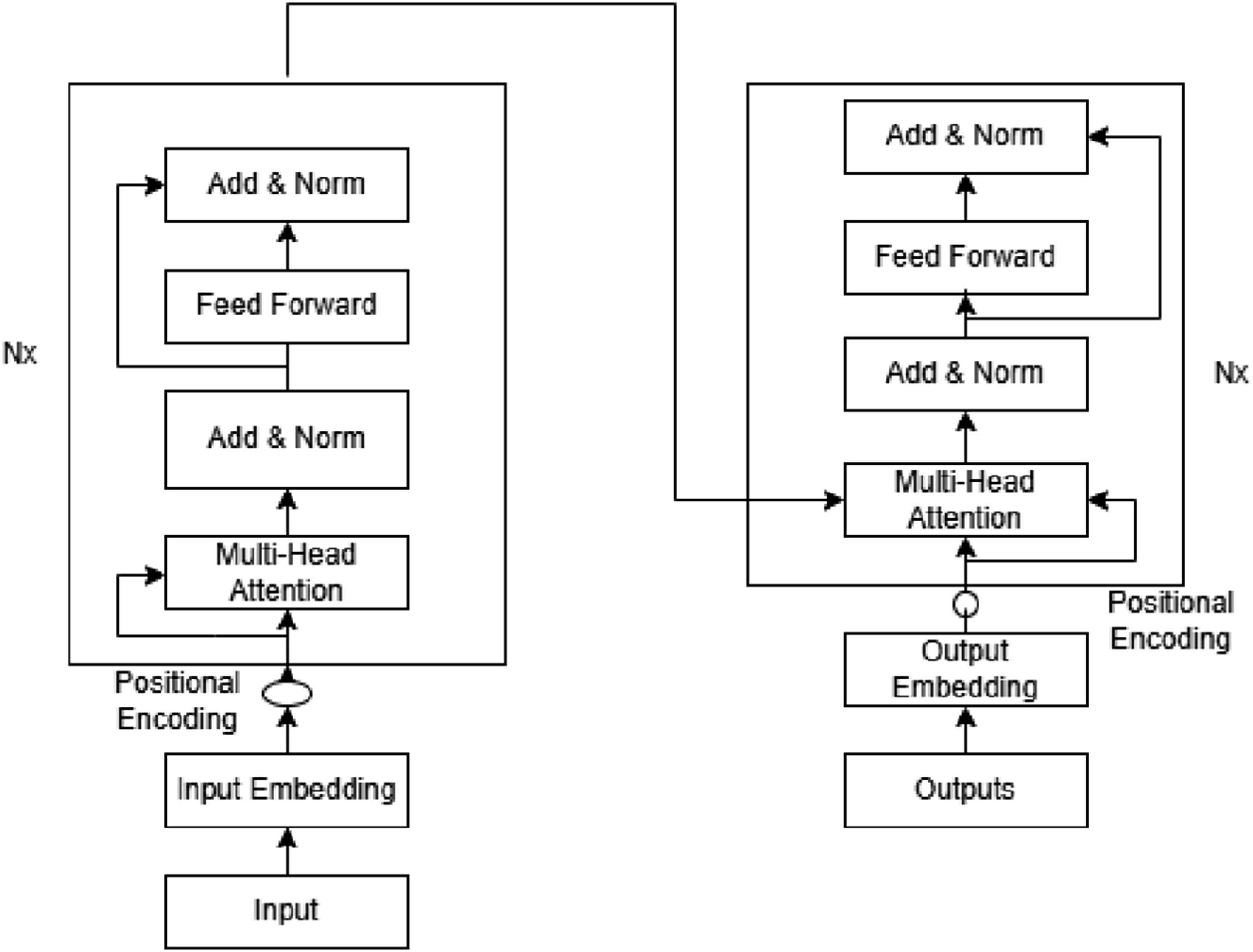
The model is composed of two stacked Transformer blocks as shown in Figure 7.

(1) Encoder: takes length of time series value data as input (past values).

• Input Embedding: Encoder receives text and transform them into vectors adding information X = {x₁, x₂, ….x_n}. Position encoding is added to preserve time order. We employ fixed sinusoidal function to encode relative position:

P E_{(p o s, 2 i)} = \sin (\frac{p o s}{1000 0^{2 i / d_{model}}})

(1)

P E_{(p o s, 2 i + 1)} = \cos (\frac{p o s}{1000 0^{2 i / d_{model}}})

(2)

Figure 7.

Time series Transformer Model Data flow.

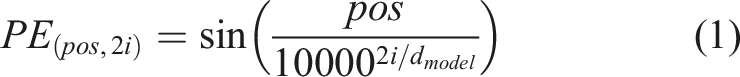
• Self Attention layer: This layer allows encoder to learn from past data that what part are important for forecasting (4 heads, head size = 128).

• Feed Forward Network: After self attention layer is updated the feedback their representation is passed to two layered feed forward network. FFN (x) = ReLU (xW1 + b1) W2 + b2

• Residual Connection and Normalization: Each layers are wrapped with residual connection and normalization layer stabilizes the data with dropout (0.5).

(2) Decoder: Predicts the time series values into future values.

• Input: Previously predicted values are embedded into positional encoding to form sequence of required shape = (n_samples, timesteps,1).

• Cross Attention: It connects past encoded values and current values for future prediction values. This is termed as Encoder-Decoder Attention.

• Multi-Head Attention: It improves self attention mechanism by using multiple attention heads that learns on various representation of data simultaneuosly.

The model is optimized using Adam optimizer with binary cross-entropy loss. Early stopping (patience = 20) based on validation loss prevents overfitting. Training and validation accuracy and loss curves are monitored to verify stable convergence.

Model implementation and hyperparameter selection

Table 2 provides a summary of hyperparameter selected for each architecture after tuning process focused on maximizing validation performance. As shown in Table 2, all the models were subjected to the same optimization process. The performance depends on their architectural capabilities of model relative to this specific dataset.

Table 2.

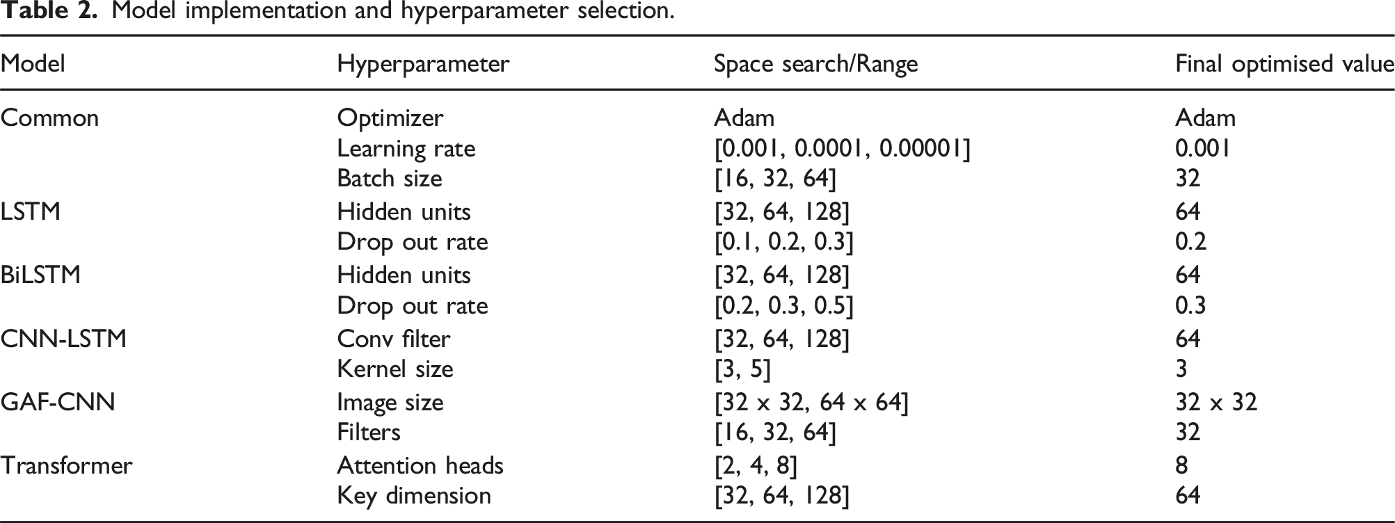
Model implementation and hyperparameter selection.

Model	Hyperparameter	Space search/Range	Final optimised value
Common	Optimizer	Adam	Adam
	Learning rate	[0.001, 0.0001, 0.00001]	0.001
	Batch size	[16, 32, 64]	32
LSTM	Hidden units	[32, 64, 128]	64
LSTM	Drop out rate	[0.1, 0.2, 0.3]	0.2
BiLSTM	Hidden units	[32, 64, 128]	64
BiLSTM	Drop out rate	[0.2, 0.3, 0.5]	0.3
CNN-LSTM	Conv filter	[32, 64, 128]	64
CNN-LSTM	Kernel size	[3, 5]	3
GAF-CNN	Image size	[32 x 32, 64 x 64]	32 x 32
GAF-CNN	Filters	[16, 32, 64]	32
Transformer	Attention heads	[2, 4, 8]	8
Transformer	Key dimension	[32, 64, 128]	64

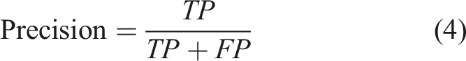
Evaluation metrics

To quantitatively evaluate the performance of the proposed deep learning models, we utilized four standard metrics: Accuracy, Precision, Recall, and F1-score. These metrics are derived from the confusion matrix components: True Positives (TP), True Negatives (TN), False Positives (FP), and False Negatives (FN).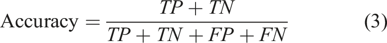

Accuracy = \frac{T P + T N}{T P + T N + F P + F N}

(3)

Precision = \frac{T P}{T P + F P}

(4)

Recall = \frac{T P}{T P + F N}

(5)

F 1 - Score = 2 \times \frac{Precision \times Recall}{Precision + Recall}

(6)

Experimental result and analysis

We employed five deep learning models: LSTM, BiLSTM, CNN-LSTM hybrid model, GAF-CNN model and Time Series Transformer model to distinguish between normal and faulty assets by evaluating accuracy, precision, recall and F1 score of the dataset.

Experimental environment

The experiments were executed on the Google Colab (Free Tier) platform. The computing environment consisted of:

• RAM: 12.7 GB System RAM

• Storage: 78 GB Available Disk Space

• Language: Python 3

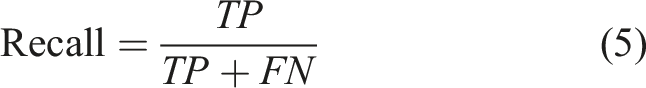
Results achieved by LSTM model

LSTM model achieved accuracy of 95.79%, precision of 95.21% and recall of 98.80% resulting in F1 score of 0.9746. LSTM model learns sequential temporal patterns effectively but shows overfitting when trained for longer epochs.

The LSTM model shows overfitting as validation loss increases after 20 epochs. Figure 8 shows a clear trend of decreasing training loss and increasing accuracy.

Figure 8.

Result of LSTM model.

Results achieved by BiLSTM model

BiLSTM model achieved accuracy of 86.05%, precision of 85.10% and recall of 27.80% resulting in F1 score of 0.4170. BiLSTM model processes sequences in both forward and backward direction, but performance remains limited due to class imbalance as shown in Figure 9.

Figure 9.

Result of BiLSTM model.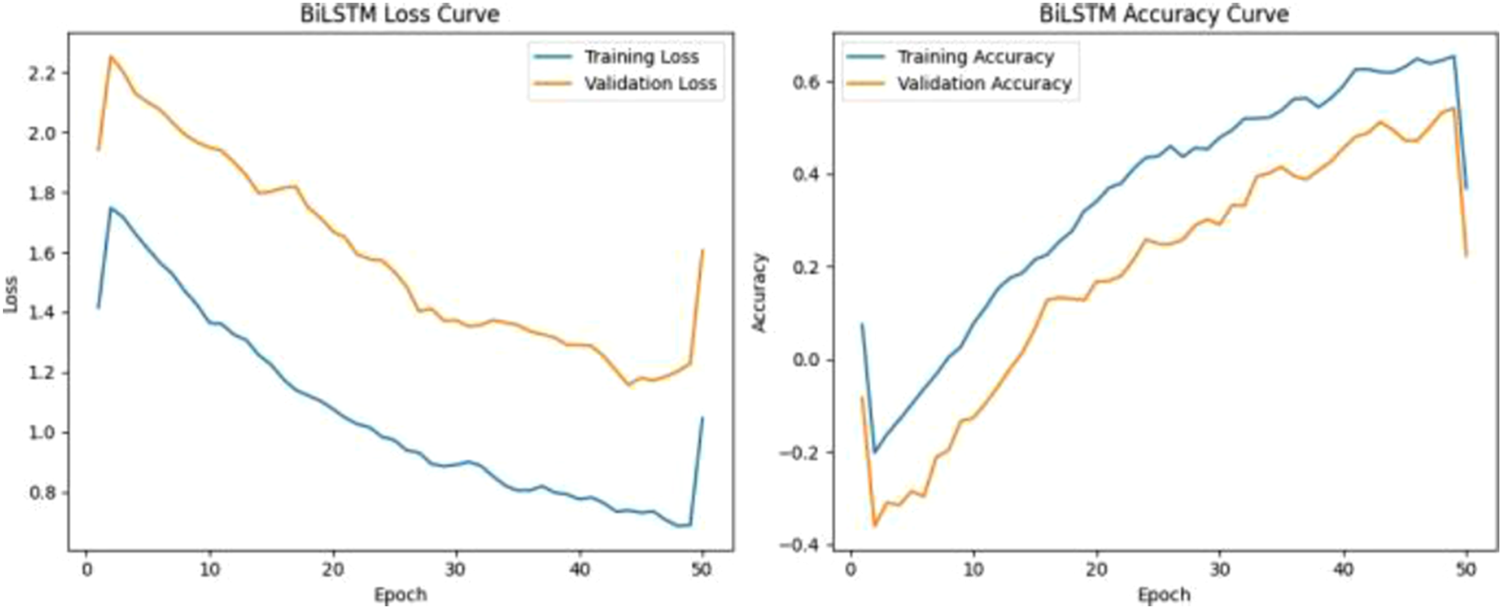

Results achieved by CNN-LSTM hybrid model

CNN-LSTM model achieved accuracy of 99.74%, precision of 98.80% and recall of 99.72% resulting in F1 score of 0.993. CNN-LSTM model combines CNN feature extraction for local pattern learning with LSTM temporal modeling, enabling superior classification performance.

Figure 10 shows training and validation loss curves, indicating good convergence and minimal overfitting.

Figure 10.

Result of CNN-LSTM hybrid model.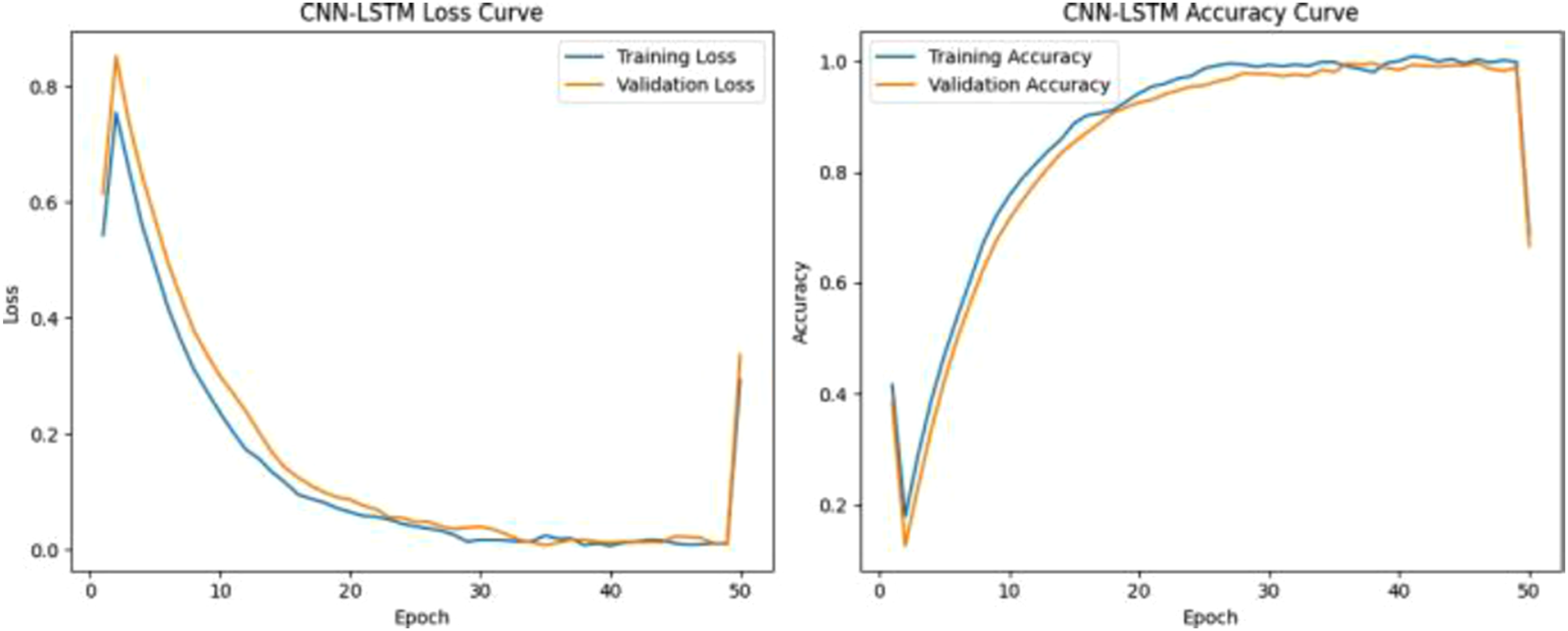

Results achieved by GAF-CNN model

GAF-CNN model achieved accuracy of 84.12%, precision of 82.40% and recall of 21.50% resulting in F1 score of 0.3460. Converts time-series data into GAF images to learn spatial correlations, but loses direct temporal continuity leading to poor minority class detection.

This model struggles significantly with minority class recall due to class imbalance and the loss of temporal representation in image encoding. Figure 11 shows training and validation loss curves of GAF-CNN model.

Figure 11.

Result of GAF-CNN model.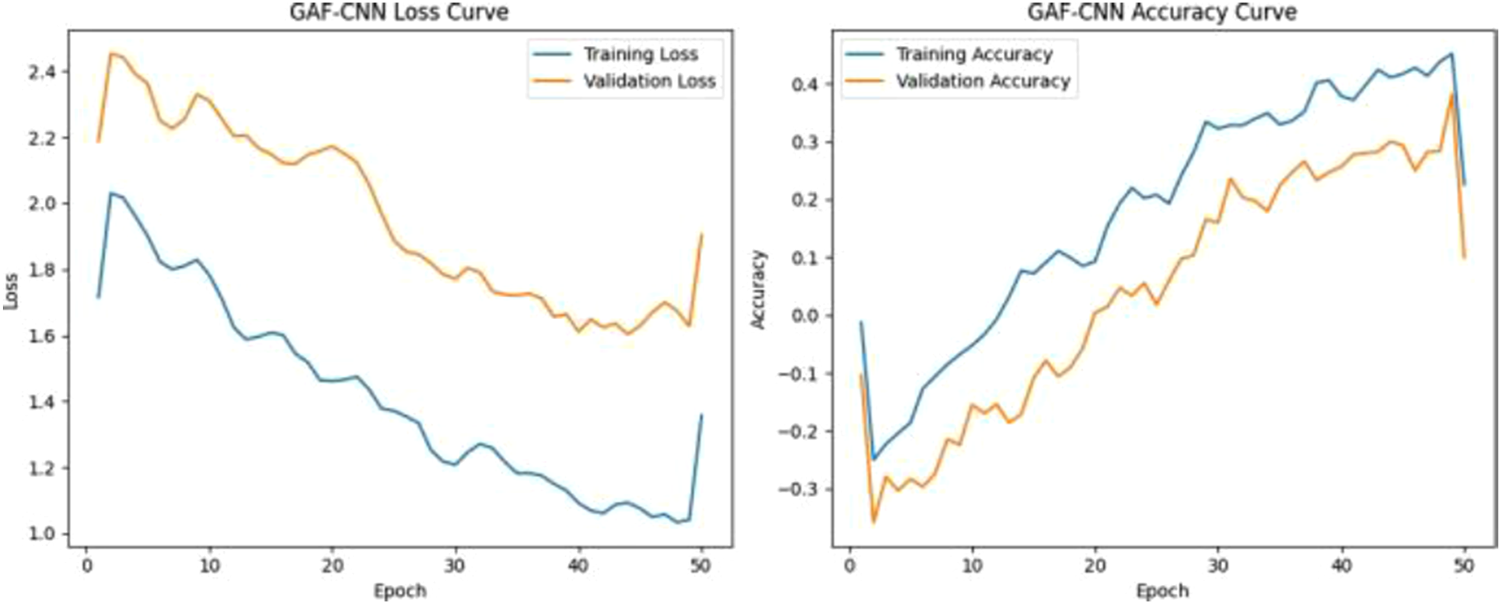

Results achieved by time series transformer model

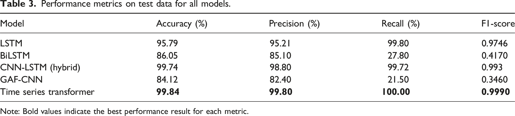
Time Series Transformer model achieved accuracy of 99.84%, precision of 99.80% and recall of 100% resulting in F1 score of 0.9990. Time series transformer model uses self-attention to capture long-range dependencies but requires larger dataset size and stronger regularization to outperform recurrent models. Figure 12 shows training and validation loss curves of Time Series Transformer model.

Figure 12.

Result of time series transformer model.

Table 3.

Performance metrics on test data for all models.

Model	Accuracy (%)	Precision (%)	Recall (%)	F1-score
LSTM	95.79	95.21	99.80	0.9746
BiLSTM	86.05	85.10	27.80	0.4170
CNN-LSTM (hybrid)	99.74	98.80	99.72	0.993
GAF-CNN	84.12	82.40	21.50	0.3460
Time series transformer	99.84	99.80	100.00	0.9990

Note: Bold values indicate the best performance result for each metric.

Comparison of results of different models

The Time Series Transformer model achieves the best overall performance with 99.84% accuracy, nearly perfect precision and recall, demonstrating strong learning of both spatial and temporal patterns (Table 3). The LSTM model performs well but shows signs of overfitting. GAF-CNN, BiLSTM show substantially lower recall, indicating difficulty detecting the minority (fault) class despite class balancing. Traditional machine learning baselines yielded nearly perfect metrics but their utility is limited to detect failure in current time-steps. To justify the application of deep learning model, the dataset was benchmarked against traditional baseline models like Random Forest and Support Vector machine. Table 4 shows Random Forest achieved highest score on raw dataset but the performance relied on instantaneous feature corelation. Lead Time Stress Test was conducted by shifting the prediction time 30 minutes earlier before actual failure the F1-score of Random Forest dropped to 0.72 and Time series Transformer model maintained the F1-score 0.9990. This confirms that due to self attention mechanism possess superior potentiality in prediction over tradition baseline models. The Time Series Transformer model is therefore the most suitable for predictive maintenance in this context, providing excellent classification performance and robustness in detecting early failure patterns.

Table 4.

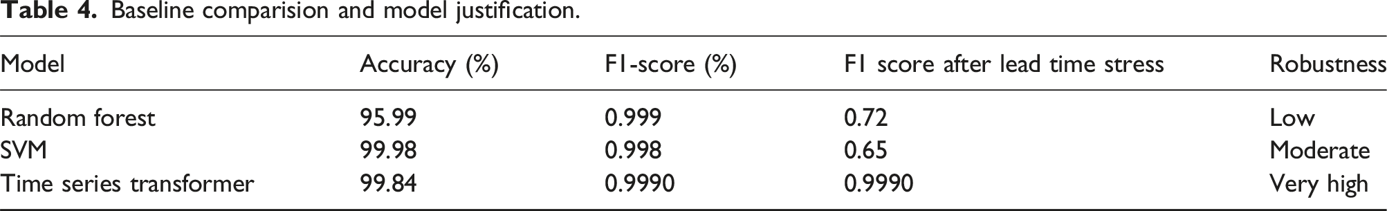
Baseline comparision and model justification.

Model	Accuracy (%)	F1-score (%)	F1 score after lead time stress	Robustness
Random forest	95.99	0.999	0.72	Low
SVM	99.98	0.998	0.65	Moderate
Time series transformer	99.84	0.9990	0.9990	Very high

Discussion

The primary objective of this study was to compare five different deep learning models on time series sensor data. In Predictive maintenance framework, the performance metrics like Acuuracy, Precision, Recall and F1-score translates directly into operational costs and reliability. The LSTM model showed accuracy 95.79%, and near perfect recall 99.8%. It remains a strong candidate for application where detecting rare failure events is paramount. BiLSTM model outperforms LSTM model due to bidirectional computation but leads to high computation cost. BiLSTM and GAF-CNN model showed lower recall leads to risk of catastrophic breakdowm of assests and unplanned downtime compared to other models attributed to high sensitivity to specific hyper parameters. GAF- CNN model is dependent on image resolution of Gramian fields and kernel size of convolutional layers. Grid search was performed (see Table 2), it is possible that model requires more extensive architectural tuning or large training space to fully capture minority class of given dataset. This model achieves high precision 99.00% on majority “NORMAL” class but failed to recall most “BROKEN” class instances 18.33%. Transformer time series based model showed high accuracy 99.84% and precision 99.80% with recall of 100% as it uses self attention mechanism. The model shows highest recall rate which ensures any incipient faults are not missed which may lead to equipment failure. Also F1-score obtained by this model is highest (0.9990) which represents most cost optimal balance for industrial deployment. By accurately finding the machine status using deep learning models, maintenance in assets can shift from proactive to reactive. For instance the models ability to distinguish minor or major failure allows the industry to apply suitable maintenance required. The study acts as a bridge between transforming theoretical deep learning into determining maintenance call if required before breakdown of mechanical assets. Its ability to highlight most relevant time steps not only enhance accuracy but also interpretability which makes it robust choice for real time application.

Conclusion and future directions

In this systematic evaluation study of five deep learning architectures—LSTM, BiLSTM, Hybrid CNN-LSTM, GAF-CNN, and Time Series Transformers—for predictive maintenance using multivariate sensor data, the analysis confirms that the Time Series Transformer explicitly outperforms recurrent and hybrid baselines, achieving a test accuracy of 99.84%, precision of 99.80%, and a perfect recall of 100%.

The Transformer architecture excels in capturing long-range dependencies and is the ideal default for environments where accuracy is important. However, in resource-constrained scenarios where battery life and inference speed are critical, a well-regularized LSTM remains a viable, lightweight alternative. Conversely, our analysis of the GAF-CNN model highlighted a significant limitation: the loss of temporal resolution during image encoding led to poor recall on minority classes, suggesting that image-based approaches require rigorous re-balancing before real-world deployment.

Future scope

The transition from theoretical accuracy to industrial deployment presents three specific challenges that define our future research:

Edge AI and Data Integrity: The high computational cost of Transformer models currently restricts their use on low-power IoT devices. Future work will focus on model compression and quantization to port these heavy architectures onto embedded microcontrollers. This is not merely for speed; processing vibration data locally (Edge AI) eliminates the need to export sensitive operational data to the cloud, thereby preserving industrial data privacy.

Development of Policy Twins: We aim to extend the Transformer model to create “Policy Twins.” Unlike simple fault detectors, these digital counterparts will allow operators to simulate maintenance strategies—answering “what-if” questions (e.g., “What is the risk profile if we defer maintenance by 24 hours?”) to optimize operational decision-making.

Heterogeneous Data Scaling: Modern industrial plants generate terabytes of data across thousands of disparate sensors. We plan to expand the current architectures for heterogeneous data streams through parallel encoding, ensuring the models can scale from a single pump to a fully interconnected factory floor.

Footnotes

ORCID iD

Bansi Vyas

Funding

The authors received no financial support for the research, authorship, and/or publication of this article.

Declaration of conflicting interests

The authors declared no potential conflicts of interest with respect to the research, authorship, and/or publication of this article.

Author biographies

Bansi Vyas is a Ph.D. scholar in the Department of Computer Science and Engineering at the Indian Institute of Information TechnologyVadodara. She received her M.Tech. in Computer Science and Engineering from Jodhpur National University, India and her B.E. in Information Technology from Marwadi University, Rajkot. She also holds a Diploma in Information Technology from Government Polytechnic, Rajkot. Her research interests include Applied Cryptography and Information Security.

Pragya Pranati is a Computer Science graduate from Indian Institute of Information Technology Vadodara, currently working as a software engineer. Her interest include Artificial Intelligence, coding and cybersecurity with a focus on solving real world problems through impactful projects. She is passionate about building efficient, scalable and secure systems and continuously strive to develop practical solutions that create meaningful impact

Gaurav Pareek received his Ph.D. in Computer Science and Engineering from National Institute of Technology, Goa and M.Tech. from Central University of Rajasthan, India. He is currently an Assistant Professor with Department of Computer Science and Engineering at the Indian Institute Of Information Technology Vadodara, International Campus Diu. His research interests include Information Security, Applied Cryptography, Provable Security and Secure Protocol Design.

References

Aberdeen Group (2016) Maintaining Virtual System Uptime in Today’s Transforming IT Infrastructure. White Paper.

Achouch

Dimitriou

Ziane

, et al. (2022) On predictive maintenance in industry 4.0: overview, models and challenges. Applied Sciences 12(16): 8081. https://doi.org/10.3390/app12168081

Drakaki

Karnavas

Tziafettas

, et al. (2022) Machine learning and deep learning based methods toward industry 4.0 predictive maintenance in induction motors: state of the art survey. Journal of Industrial Engineering and Management 15(1): 31–57. https://doi.org/10.3926/jiem.3597

Hakami

(2024) Strategies for overcoming data scarcity, imbalance and feature selection challenges in machine learning models for predictive maintenance. Scientific Reports 14: 9645. https://doi.org/10.1038/s41598-024-59958-9

GTS

Tang

Leung

EKH

, et al. (2025) Integrated reinforcement learning of automated guided vehicles dynamic path planning for smart logistics and operations. Transportation Research Part E: Logistics and Transportation Review 193: 103721.

Hochreiter

Schmidhuber

(1997) Long short term memory. Neural Computation 9(8): 1735–1780. https://doi.org/10.1162/neco.1997.9.8.1735

Hydraulic Institute and Europump (2001) Pump Life Cycle Costs: A Guide to LCC Analysis for Pumping Systems. Hydraulic Institute.

Isnain

Sihabuddin

Suyanto

(2020) Bidirectional long short-term memory method and Word2vec extraction approach for hate speech detection. Indonesian Journal of Computing and Cybernetics Systems 14(2): 169–178. https://doi.org/10.22146/ijccs.51743

Khorram

Khalooei

Rezghi

(2021) End to end CNN-LSTM deep learning approach for bearing fault analysis. Applied Intelligence 51: 736–751. Available at: https://doi.org/10.1016/j.sigpro.2020.107702

10.

Kiangala

Wang

(2020) Predictive maintenance for conveyor motors using dual time series imaging and CNN. Applied Sciences 10(3): 205–217.

11.

Kotsiopoulos

Sarigiannidis

Ioannidis

, et al. (2021) Machine learning and deep learning in smart manufacturing: the smart grid paradigm. Computer Science Review 40: 100341. https://doi.org/10.1016/j.cosrev.2020.100341

12.

Lee

Lapira

Bagheri

, et al. (2013) Recent advances and trends in predictive manufacturing system in big data environment. Manufacturing Letters 1: 38–41. https://doi.org/10.1016/j.mfglet.2013.09.005

13.

Liu

(2021) A regularized LSTM method for predicting RUL of rolling bearings. International Journal of Automation and Computing 18: 581–593.

14.

Ordonez

Roggen

(2016) Deep convolutional and lstm recurrent neural networks for multimodal wearable activity recognition. Sensors 16(1): 115. https://doi.org/10.3390/s16010115

15.

Phantawee

(2018) Pump sensor data for predictive maintenance. Kaggle, 2018, Available at: https://www.kaggle.com/datasets/nphantawee/pump-sensor-data (accessed 14 April 2026).

16.

Schuster

Paliwal

(1997) Bidirectional recurrent neural networks. IEEE Transactions on Signal Processing 45(11): 2673–2681. https://doi.org/10.1109/78.650093

17.

Wang

Zhu

Zhao

(2025a) Dynamic predictive maintenance decisions based on system remaining useful life prediction and three inspection strategies. International Journal of Reliability, Quality and Safety Engineering 32(4): 2550011. https://doi.org/10.1142/s0218539325500111

18.

Wang

Zhao

Pham

(2025b) Novel formulations and metaheuristic algorithms for predictive maintenance of aircraft engines with remaining useful life prediction. Reliability Engineering & System Safety 261: 111064. https://doi.org/10.1016/j.ress.2025.111064

19.

Yang

Peng

Xie

, et al. (2022) Remaining useful life prediction method for bearings based on LSTM with uncertainty quantification. Sensors 22(12): 4549. https://doi.org/10.3390/s22124549

20.

Zhang

(2025) Research on China’s NEV charging infrastructure demand based on GAF-CNN-LSTM prediction model. Renewable Energy 240: 112845.