






Abstract
We revisit a critical problem of cross-cultural research: the non-independence of nations arising from shared ancestry and joint cultural diffusion. Recent review highlighted that few published cross-cultural studies attempt to control for such non-independence, often doing so inefficiently. This may compromise causal claims derived from such analyses. We reassess the problem and caution against using a one-size-fits-all “remedy” for non-independence. Non-independence can involve three distinct issues—(1) confounding by (un)observable variables, (2) Galton’s problem (joint diffusion and shared ancestry) as a special case of confounding, and (3) non-independence as a nuisance—each requiring a careful assessment of the causal model and a specific treatment. Controlling for non-independence by default may result in one of five outcomes, including successful elimination of the bias, improving precision, doing nothing, harming precision, or introducing bias, which we demonstrate with simulations. Instead of rolling a five-sided dice, we encourage cross-cultural scholars to begin with a careful evaluation of their underlying theoretical assumptions and causal models. In essence, we contribute to the refinement of cross-cultural research methodology by advocating for a tailored approach to addressing non-independence that models the real-world processes under examination.
Nigeria. Malaysia. Singapore. Myanmar. Australia. These five countries seem distinct from each other in cultural beliefs and practices. To understand why these countries are different, one might consider the influence of differences in various geographical and ecological factors (e.g., climate, land size, natural resources). However, a common scientific argument is that in understanding cultural differences connected to political histories (e.g., government structure), these five countries should not statistically be treated as five countries, but one “cluster”. This is because all five countries were, at some point in their history, British colonies. This is, in essence, an example of the problem of non-independence.
The problem is well-known in anthropology and ecology (Mace et al., 1994), and recent work by Claessens and colleagues (2023) revisits this significant methodological challenge in cross-national research. The authors argue that many studies fail to adequately consider in their statistical analysis how countries are interconnected by geography and shared ancestry. As researchers often falsely treat countries as independent of each other, their findings could be biased, increasing the frequency of Type I errors (false positive results). By reviewing top publications in cross-cultural research, their study shows that many findings change when these connections are accounted for, calling for future research to adopt more robust methods.
The problem of non-independence is a complex one. Despite having been recognized for centuries, a widely agreed-upon methodological remedy has not been adopted. Here, we seek to build on existing discussion of this issue, highlighting that (1) controls for spatial and/or linguistic similarities may misrepresent the true underlying issues, (2) the problem of non-independence is in fact more heterogeneous than it looks, and depending on the nature of the problem, (3) statistical controls without careful thought, both when dealing with non-independence or tackling confounds more broadly, may lead to biased research findings. In doing so, we use the points made in Claessens et al.’s work as a reference, due to being the most recent and salient revival of this discussion. The insights and findings hold significant relevance for scholars who wish to enhance the rigor of their cross-cultural analyses. The authors’ contribution opens up the opportunity to introduce a few additional issues that deserve attention.
In this article, we systematically assess the problem of non-independence and study various scenarios of how it could arise. In each of them, we look at the impact of controlling for non-independence 1 , also using empirical simulations. These examples are simplifications for illustrative purposes only and are not intended to be irrefutable but mostly to compel researchers to think about their underlying causal models. Our overarching goal is to promote accuracy of causal inference in cross-cultural research by addressing bias, defined as the systematic deviation of an estimated effect from the true causal effect (Cinelli et al., 2022).
Reassessing the Evidence for Non-Independence in Cross-National Research
As noted earlier, the problem of non-independence has been known for centuries but remains overlooked by the research community. Why might this be so? It seems straightforward that countries that are geographically close and/or that share the same language have shared histories, and this needs to be controlled for (Claessens et al., 2023). That said, the nature and the solution to the problem may be more complex than they appear at first glance.
Claessens et al. (2023) highlight spatial and linguistic relatedness as key drivers of cross-national variation in economic and cultural values. The authors demonstrate that a substantial proportion of the variation in key economic and cultural indicators, widely used in cross-cultural research, can be “explained” by geographic proximity (e.g., around 75% in Gini Index) and shared cultural ancestry (e.g., around 75% in Individualism). They conclude “that economic development and cultural values are spatially and culturally non-independent across nations, emphasising the need to control for non-independence” (p. 2). However, the use of zero-order correlations as a basis for such a conclusion overlooks the complexity of causal relationships that transcend mere spatial or linguistic commonalities.
In similar analyses examining the predictors of cultural similarity between 40 European countries, linguistic proximity and geographic distance do account for 13% and 23% of the cultural distances between countries, respectively (Akaliyski, 2017). However, in multiple regressions with several other theoretically plausible predictors of cultural similarity 2 , the effect size of sharing a language family on cultural distance diminishes by about 74% (from −28.48 to −7.33), and that of sharing the same language by about 54% (from −41.30 to −18.99), whereas that of geographic distance completely vanishes. Thus, knowing that a national indicator clusters geographically does not allow us to conclude that it has been spatially diffused because the spatial clustering can be due to multiple other factors. For example, Scandinavian countries have similar cultures, they are also neighboring each other and speak similar languages. We may jump to the conclusion that their cultural characteristics have been transmitted from their shared ancestors, such as the Vikings. However, they also share similar climates, religion, history, level of socio-economic development, and political institutions, all of which may be the true causal explanation for their cultural similarities (and not their geographic proximity and shared ancestry). Geographic proximity and shared ancestry indeed typically correlate with cultural similarity but this relationship can often be spurious. Processes of cultural inheritance and geographic diffusion may also follow different patterns; for instance, practices like sea fishing are typically transmitted within coastal communities across generations but do not diffuse inland geographically, whereas phenomena like disease prevalence can spread across geographic space without implying cultural inheritance.
To “replicate” a dozen highly-cited studies that did not control for non-independence, Claessens et al. (2023) estimated bivariate correlations (aside from two cases where they included one control variable, see their Figure 5). When they added controls for spatial and linguistic dependence, the reduction in the correlation strength was relatively modest but half of the correlations no longer remained significant at the 95% confidence level. From a causal point of view, though, these demonstrations do not prove any reduction in bias since the controls for independence may simply capture the variation in other confounders that scholars usually account for in their studies, but Claessens et al. (2023) did not, or they may also control for mediators or induce collider bias (see below). These oversights remind us of the necessity to evaluate the underlying causal models in cross-national research to ensure a credible interpretation of typically complex socio-cultural relationships.
The Nature of Non-Independence of Nations
Undeniably, the problem of non-independence exists, but it requires precise specification. Galton’s problem, or the problem of non-independence of cultural units, occurs when our predictor and outcome are diffused or inherited by shared ancestry and therefore the relationship we find between them is not causal but spurious (Naroll, 1965). In this sense, the problem of non-independence is simply a special case of the general problem of endogeneity, induced by third variables (confounds).
Types of Non-Independence Problems and Suggested Solutions
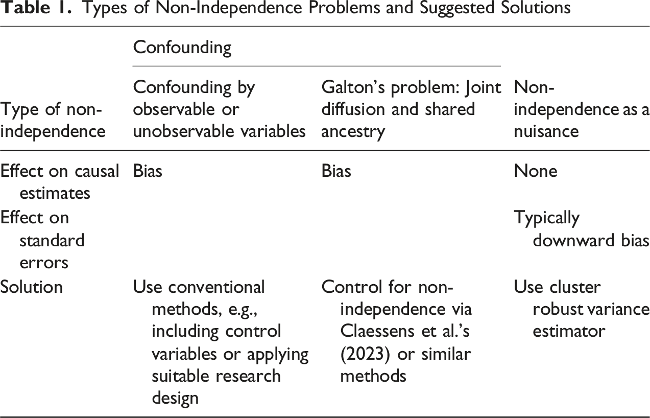
First is the problem of confounding by observable or unobservable variables such as climate or shared histories of colonialism and post-communism. Peer-reviewed cross-cultural research interested in identifying causal relationships rarely neglects adjustment for or discussion of (residual) confounding where that is necessary and possible. Using fixed effects for measured covariates has an advantage over using random effects for cultural clusters or relatedness: It avoids the “incomplete conditioning” problems (Hazlett & Wainstein, 2022) that come with shrinkage-based methods like that by Claessens et al. (2023), which may not fully capture the confounding influences. If observable, using direct measures of the confounder(s) should be the preferred way to control for their impact rather than using proxies such as geographic proximity and linguistic similarity as proposed by the authors. For instance, if a researcher is interested in cross-country variation in legal policies as an outcome, instead of simply controlling for shared colonial histories, one might instead control specifically for the extent/duration during which a country adopted a colonizer’s legal systems. The selected variables should suit the research question and causal model at hand. We return to this case in our section “Mediated Confounding”. Besides regression adjustment, quasi-experimental designs are an option for causal inference about cultural variables, even in the presence of unobserved confounding (see, for example, Faessler et al., 2023; Wang et al., 2023).
Non-independence as a nuisance is a second problem that falls within the same umbrella of issues related to non-independence of nations, albeit of quite a different nature. In some settings, the causes of non-independence might not be of particular relevance for the research question and dependence may hence not bias the effect estimates. For example, in a study on the effects of trade liberalization on income inequality across countries, non-independence may become a nuisance when countries influenced by shared economic treaties exhibit similar inequality trends. Yet, we might not want to condition on membership in the treaty, because our target estimand (i.e., the effect we aim to estimate) is the marginal effect among countries – not the effect for a given treaty cluster. If we control for treaty membership, we would be estimating how trade liberalization affects inequality for countries within the same treaty (conditional effect) instead of understanding its population-average impact across all countries, regardless of treaty status. Hence, whether or not we control for treaty membership effects depends on our research question: if we are interested in the average relationship between trade liberalization and inequality across all countries, having treaty cluster membership as a term in the model would not yield the estimate we are interested in. Rather, non-independence of countries in this scenario merely induces pseudo-replication, effectively reducing the amount of information per data point. We can correct for it with conventional cluster robust standard error estimators (Liang & Zeger, 1986), or Conley standard errors, if suitable distance measures are available (Conley, 1999). Such corrections take into account heterogeneity across clusters and distances when estimating the error of our effect estimator.
The third form, Galton’s Problem, is a particular case of confounding, named after Sir Francis Galton, who highlighted the challenge of non-independence in comparative cultural data, acknowledging that cultural traits can be diffused 3 . Naroll (1965) specified Galton’s problem as arising when we have a joint diffusion. That is, both the predictor (X) and the outcome (Y) are diffused or inherited (Z). For example, one might hypothesize that in populations high in density, a jury system is more likely to emerge (given the requirement for a large pool of individuals, unrelated to the defendant, who can be drawn upon). Even if a relationship between the two is found, this could be a problem of joint diffusion. In this case, countries that were colonized by the British might have both (1) adopted infrastructural practices and technology that allow a large population, and (2) adopted common law, including a jury system. If so, then it is not population density of countries (X) that led to the emergence of jury systems (Y), but a shared colonial history (Z). The key issue Naroll (1965) presents is distinguishing between “historical” and “functional” associations in cross-cultural research. Researchers typically wish to make claims about a functional association: X causes Y. But diffusion or shared ancestry (Z) can be the source of both, creating a historical form of association, which is spurious.
However, we want to draw readers’ attention to the fact that simply having an association structure between X, Y, and Z, does not reveal whether the link is historical, functional, or a combination of both. We need a causal model to determine whether confounding that biases our causal estimates occurs and needs to be taken care of.
Causal Models with Controls for Spatial and Linguistic Dependence
Theoretical Models
The spurious-type relationship Claessens et al. (2023) depict is plausible and a valid concern. However, this should not be portrayed as the causal model, overlooking a myriad of possible causal relationships involving other observable or unobservable variables, of which the spurious correlation is just one example, not necessarily the most common one. Figure 1 presents five such models where X is a cause of Y, the outcome of interest. In all cases, we are interested in the causal effect of X on Y. A third variable (or variables) Z denotes a potential confounder.
4
Model 1 shows a classic case of a confounded X-Y relationship due to shared cause Z, which requires controlling for Z to obtain unbiased X-on-Y estimates. In Model 2, where Z affects only Y, controlling for Z is optional but can enhance precision by accounting for Y’s variation not explained by X (Cinelli et al., 2022). Model 3, with Z unrelated to X and Y, makes controlling Z irrelevant. Model 4 presents Z as a background variable for X, unrelated to Y. Here, controlling for Z is unnecessary and could lead to larger standard errors and potential Type II (false negative) errors, as it reduces exogenous variation in X that creates variation in Y (Cinelli et al., 2022). Model 5 introduces an unobserved confounder U into the previous model, affecting both X and Y, and thus creating a partly spurious correlation. Controlling for Z here exacerbates the bias from U, as it diminishes X’s variation due to the external variable Z that is not a confounder (Cinelli et al., 2022). Examples of Simple Types of Causal Models Involving Third Variables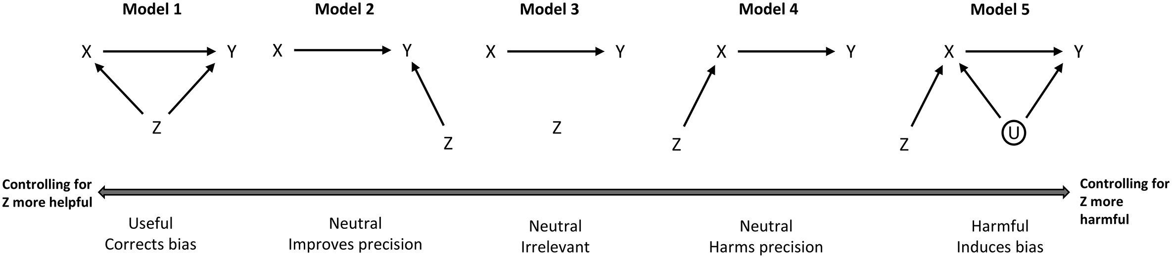
A cautious researcher can provide many examples of a possible Model 1. For instance, the relationship between religiosity and economic development may be confounded because religious traditions often spread through historical and regional ties rather than independent societal choices (Ruck et al., 2018). Many predominantly Catholic countries in Latin America have similar levels of religiosity and economic development, not necessarily because religion affects economic growth, but due to shared colonial histories, church-state relations, and regional economic trends. Thus, controlling for Z would ensure we obtain unbiased estimates of the effect of X on Y (assuming no other sources of confounding exists).
For Model 2, we may be interested in the relationship between climate (X) and emancipative values (Y) (e.g., Welzel, 2013). Controlling for shared linguistic ancestry or geographic proximity (Z) may improve precision but it is not necessary for obtaining an unbiased estimate of X on Y. While Welzel’s theory proposes causal mechanisms through which climate causes emancipative values—cooler climates with continuous rainfall provide the conditions for independent farming which foster stronger emancipative values—countries that share a common linguistic heritage (e.g., Romance or Germanic language families) may also have similar levels of emancipative values due to historical diffusion of cultural norms. However, since it is impossible for linguistic ancestry or geographic location to causally affect climate, controlling for it is unnecessary for unbiased estimates of the effect of X on Y. As it reduces unexplained variance in Y, accounting for shared ancestry could nevertheless increase precision.
Model 3 requires strong assumptions that spatial and linguistic dependence do not affect either X or Y. Claessens et al. (2023) have replicated one such case: the relationship between natural disaster vulnerability (X) and tightness-looseness (Y) as proposed by Gelfand et al. (2011). Arguably, this applies only to spatial dependence (Z) though since spatial dependence cannot possibly influence the occurrence of natural disasters 5 and Claessens et al. (2023) demonstrate that tightness-looseness does not exhibit spatial patterning. Thus, controlling for spatial dependence would be completely irrelevant – we also see that it does not alter the estimated coefficient of natural disaster vulnerability in Claessens et al.’s demonstration (their Figure 5, p. 7). 6
For Model 4, consider the following example: Research suggests collectivism (X) predicted nations’ likelihood of mask-wearing during the COVID-19 pandemic (Y) (Lu et al., 2021). Imagine a genetic factor (Z), representing shared cultural ancestry, that hypothetically affects collectivism but not mask-wearing directly. In this scenario, not controlling for shared ancestry would still yield an unbiased estimate of the effect of collectivism on mask-wearing. Controlling for it might instead introduce imprecision, potentially leading to a false negative relationship between collectivism and mask-wearing.
To transition this into the bias-inducing Model 5 type scenario, consider introducing an unmeasured fourth variable that affects both collectivism and mask-wearing, such as perceived pathogen threat. In that case, controlling for shared cultural ancestry (Z) would bias the true causal relationship between X and Y, increasing the risk of Type II errors. It is, thus, to be avoided.
Empirical Illustrations with Simulations
To demonstrate the practical implications of different causal models, we conducted simulations to evaluate the implications of controlling for a third variable (Z) across the five causal scenarios, each representing a different causal structure involving the predictor (X), outcome (Y), and third variable (Z). While these causal models are well known in the causal inference literature and can be derived analytically (Cinelli et al., 2022; Elwert, 2013; Pearl, 1995), we conduct these simulations to illustrate the implications in a manner accessible to cross-cultural researchers, using parameters calibrated to the effect sizes, confounding strengths, and sample sizes commonly observed in cross-national studies. In each scenario, we generated simulated datasets of X, Y, Z, and U, where applicable, by first drawing all nodes without parents (e.g., node Z in Model 1) from standard normal distributions. All descendant nodes (e.g., node Y in Model 1) were formed as a weighted sum of all their parent nodes, with subsequently added independent, normally distributed noise. The weights for these linear combinations and the noise variances were chosen to achieve the desired covariance structure implied by the theoretical model and the true effect sizes of the simulation scenario. Furthermore, they were chosen so that all simulated random variables had a theoretical mean of zero and a variance of one, reflecting the standardized predictors and outcome variables typically used in applied research. As a consequence, all effect sizes in our simulations (true and estimated) can be understood as standardized linear regression coefficients. We systematically varied sample sizes (30, 60, 120 countries), the true causal effect of X on Y (linear regression coefficients of 0, 0.3, 0.5), and the strength of the effects of Z on X and/or Y (0.3, 0.6). In Model 5, an unobserved confounder (U) was added as a latent common cause of both X and Y, with effect size set to the same value as Z’s effect on X (0.3 or 0.6). The effect sizes represent standardized regression coefficients in a linear additive model. When a variable had multiple parent nodes (e.g., X and Z), we added a single normally distributed noise term and scaled it such that all variables had unit variance.
For each model, we estimated regression models with and without controlling for Z, allowing us to evaluate whether inclusion of Z improved accuracy, harmed precision, or introduced bias. We skipped Model 3 because, since Z is unrelated to any of the other two variables in that model, the results with and without control for Z would be identical. In each simulation, we estimated the effect of X on Y using linear regression, with Z included as a covariate where applicable. Each point plots the average estimated coefficient on X over 1000 simulations for a given combination to ensure stable estimates. All analyses and data visualizations were conducted in R (R Core Team, 2025). All simulation code is publicly available in a GitHub repository: https://github.com/Akaliyski/non-independence.
In Figure 2, we present 36 averages of the predictor’s resulting causal effect, one for each scenario and Model in Figure 1. Of note is that the actual possible combinations of parameter values are virtually indefinite even in such simple models without considering further variables. Moreover, the actual empirical models researchers deal with in their analyses are usually far more complex than these simulations, while still being simplifications of the real world. Therefore, our simulations serve as simple illustrations rather than a comprehensive guide to researchers. They should be taken with caution. Simulation Results Illustrating the Implications of Controlling for a Third Variable (Z) Across Four Causal Models. Notes. The Plots Display Estimated Regression Coefficients for X Predicting Y, With (Green) and Without (Blue) Controlling for Z, where Applicable. True Causal Effect Sizes are Indicated by Horizontal Dashed Lines (b, True Effect Size = 0, 0.3, 0.5). The Strength of Z’s Associations (True Effect Size = 0.3 or 0.6) With X And/or Y, and Sample Sizes (n = 30, 60, 120), are Systematically Varied. In Model 1, “Conf” Refers to the Strength of the Association Between Z on the one Hand and X and Y on the Other. In Model 2, Path “C” is the Association Between Z and Y. In Model 4, Path “a” is the Association Between Z and X. “Conf” in Model 5 Refers to the Strength of the Confounding From U on Both X and Y, as Well as the Strength of the Association Between Z and X. Each Point Plots the Average Estimated Coefficient on X Over 1000 Simulations for a Given Combination to Ensure Stable Estimates. Error Bars Represent the Means of the Lower and Upper 95% CIs Across Simulations. Coefficients Falling on the Dotted Lines are Unbiased. The Further away From the Dotted Line, the Stronger the Bias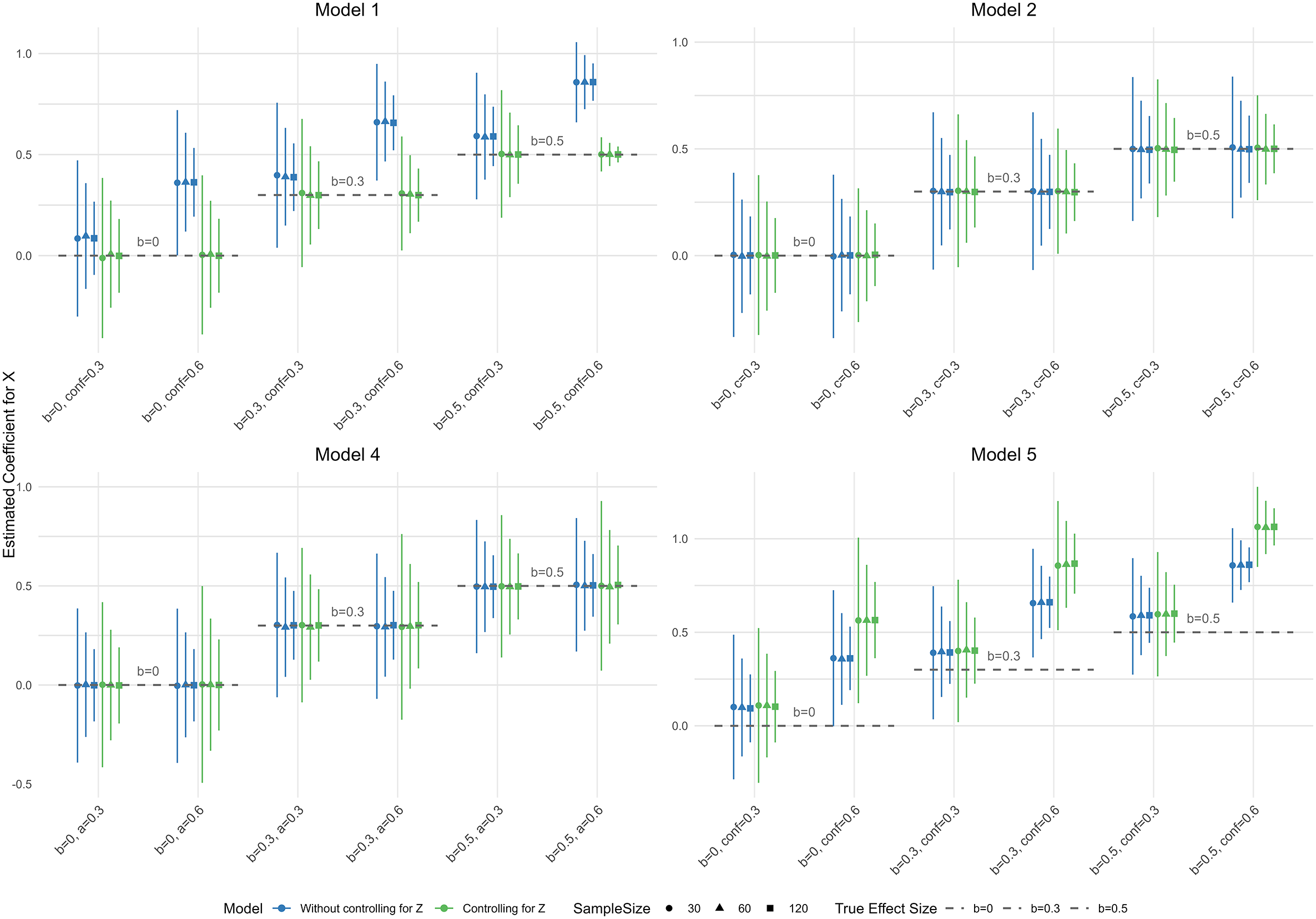
All results are as expected, according to Figure 1. In Model 1, controlling for Z results in unbiased estimates of X on Y regardless of the true effect, confounding, and sample sizes. Unsurprisingly, controlling for Z (green lines) here corrects the biased/inflated estimates of X’s zero-order effect (blue lines), bringing it back to its unbiased/true effect (horizontal dashed line). This is especially so when Z's effect size on X and Y is larger. A Type I error occurred only in the case where the true effect (b), the confounding (conf), and the sample size (n) were all small (b and conf = 0.3, n = 30).
In Model 2, we observe unbiased estimates in all cases but the confidence intervals were narrower when controlling for Z. The difference in the width of the confidence intervals was barely noticeable when the effect size of Z on Y was small (c = 0.3), but more substantial when that effect size was larger (c = 0.6). For example, when b = 0.3, c = 0.6, and n = 30, we obtain a Type II (false negative) error without controlling for Z, which is not the case when Z is controlled for. Hence, in situations like Model 2, taking third variables into account can allow researchers to capture a significant predictor, when error makes it seem like there is no effect.
Model 4, however, concretely highlights how controls for Z can go wrong. When Z is associated with X (but not Y), controlling for Z leads to wider confidence intervals. This is particularly obvious when Z has a higher effect size on X (a = 0.6). For example, at b = 0.3, c = 0.6, and n = 60, where X’s effect is significantly greater than zero X becomes a non-significant predictor when Z is controlled for due to the widened confidence intervals. Hence, controlling for third variables in such situations can lead to Type II errors.
In Model 5, the problem gets worse. When Z is associated with X (but not Y) and there is an unobserved factor U that is associated with both X and Y, controlling for Z actually leads to an inflated estimate of X’s effect. This can be particularly problematic when X has no true effect. For example, at b = 0 (X has no effect), conf = 0.6, and n = 30, a previously (accurately estimated) null effect of X actually becomes significant (different from zero) after controlling for X. We obtain biased estimates in all cases. However, they are significantly more biased when we control for Z, especially when the confounding by the unobservable factor U was stronger.
Since Claessens and colleagues reported that spatial and linguistic “dependence” can exceed even a correlation of 0.6, we repeated our models also with confounding strengths of 0.75 and 0.85. These models, presented in Figure S1 in the Supplemental Material, show greatly inflated confidence intervals in all cases, indicating a high risk of Type II error. This is the case especially in Model 4, where a moderate true effect (b = 0.5) remains not statistically significant even when the sample size is fairly large (n = 60) if we control for Z. These findings should serve as a caution against including third variables indiscriminately, especially with small sample sizes, which is commonly the case in cross-cultural research.
Collider Bias
For brevity and readability, the models in Figure 1 and Figure 2 only consider Z as a parent node, i.e., it is a (potential) predictor of X and/or Y. However, although arguably rare, models where Z is a descendant are also conceivable. This would lead to conditioning on post-treatment variables – i.e., collider bias – which opens further dangers for model misspecification. Consider a scenario where economic modernization (X) influences democratic values (Y) directly (Inglehart & Welzel, 2005), but both economic modernization and democratic values independently promote greater cultural diffusion (Z). For instance, wealthier countries may have more resources for global cultural engagement (Tomlinson, 1999), while democratic countries may actively spread democratic norms among each other (Deutsch & Welzel, 2016). Consequently, diffusion (Z) becomes a collider—an endogenous descendant influenced by both X and Y. In this scenario, controlling for Z, intended to account for non-independence, inadvertently induces collider bias, creating or distorting statistical associations and thus biasing the estimate of the true causal effect of economic modernization on democratic values.
Figure 3 (Model 6) illustrates this case with a simulation in which we generate three variables—X, Y, and Z—across multiple scenarios, then estimate two regression models (with and without controlling for Z). First, X is drawn from a standard normal distribution, and Y is created so that it depends on X plus random noise, while ensuring Y has a constant variance. Next, Z is introduced as a “collider” that partly depends on X and Y, making it a post-treatment variable. We vary the true effect of X on Y (true effect size = 0, 0.3, 0.5), the collider strength (i.e., the coefficients for the links Z→X and Z→Y in the data-generating model, set at either 0.3 or 0.6, for both), and sample sizes (30, 60, 120), repeating each simulation 1000 times. Collider Bias in Simulations of Cross-National Analyses. Notes. The Predictor (X) is Drawn From a Standard Normal Distribution and the Outcome (Y) is Generated as a Function of X Plus Noise, while Ensuring Constant Unit Variance. The Collider Variable (Z) is Constructed as a Weighted Combination of the Difference (Y – X) and Random Noise Such that Z has Unit Variance as well. The More Weight is Put on the Difference (Y – X), the Higher the Effect Size of Z on Y, and the Negative Effect of Z on X, i.e., the Stronger the Colliding. We Vary the True Effect of X on Y (True Effect Size = 0, 0.3, 0.5), the Collider Weight (True Effect Size = 0.3, 0.6), and the Sample Size (30, 60, 120). Two Regression Models are Estimated: one Regressing Y on X Alone and a Second Controlling for Z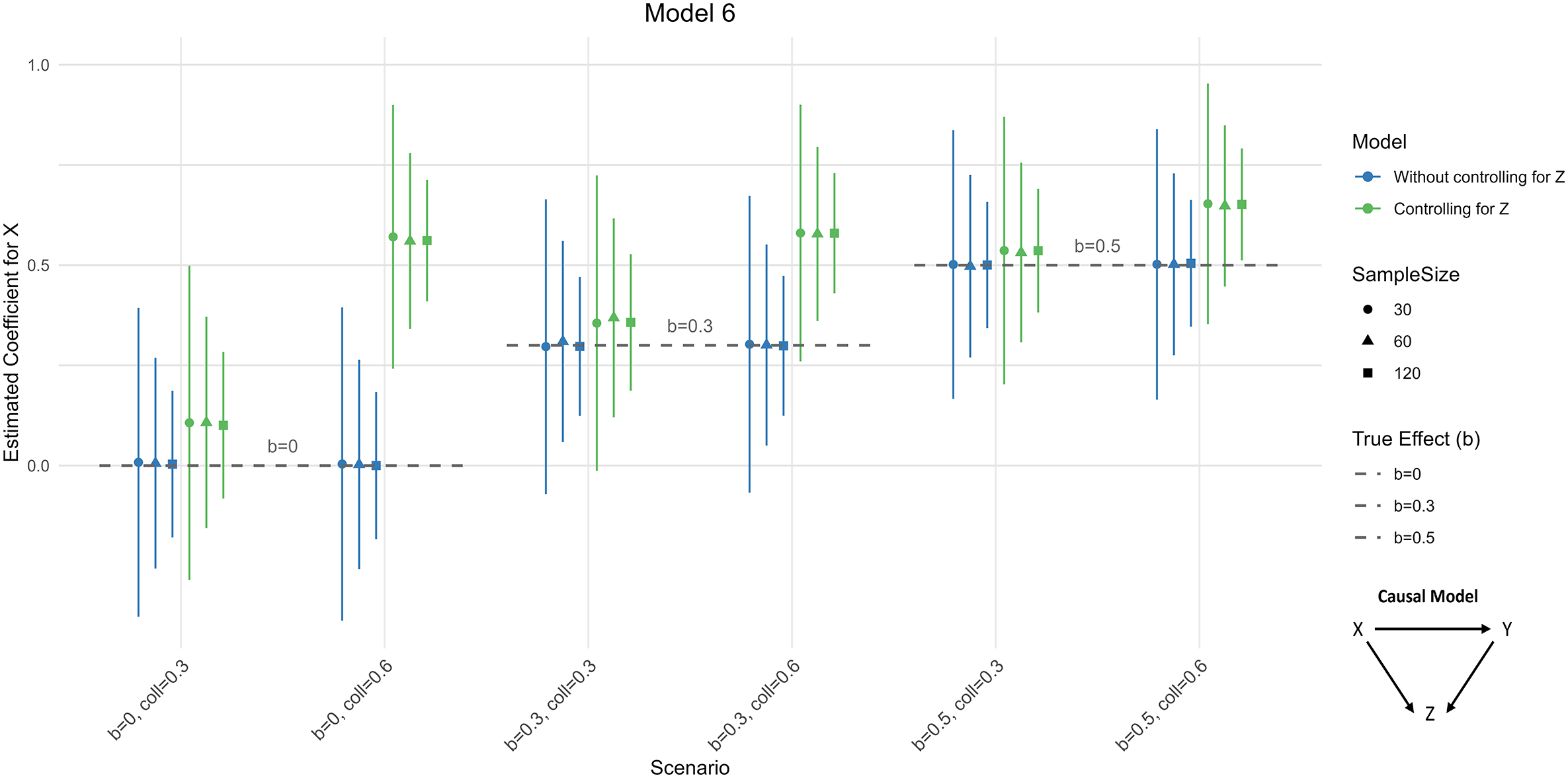
As shown in Figure 3, the model that excludes Z accurately recovers the true causal effect of X on Y, whereas controlling for Z—the collider—leads to a positively biased estimate of X’s coefficient. The bias becomes stronger, the lower the true causal effect of X on Y and the larger the colliding association (that between X and Z and Y and Z). In purely cross-sectional observational analyses, the pattern of associations among X, Y, and Z alone is insufficient to distinguish whether Z serves as a confounder or a collider—whether Z causes X and Y or is caused by them can only be determined theoretically, not statistically. Put another way, without a clear theory and causal model, blindly controlling for third variables can lead to “discovery” of an effect, even when there is none.
Therefore, without knowing the real causal relationships between variables, we may as well introduce bias instead of removing it. Controlling for shared ancestry and spatial autocorrelation is necessary only if we are certain that we are dealing with a Model 1, and possibly also Model 2, type of relationship. Even in that scenario, where confounding exists, one needs to define what the source of that confounding is—diffusion, shared ancestry, or something else—and apply appropriate adjustments to make sure no harmful controls are introduced into the model.
Mediated Confounding
Furthermore, we make a broader point: diffusion or ancestry typically affect contemporary outcomes through intermediate pathways, rather than directly as suggested by our Models 1-6. In such cases, it is advisable to control for those mediators—whenever observable—rather than rely on coarse proxies like spatial or linguistic distance, which also open the possibility of unintentionally introducing bias. Consider a case where historical cultural diffusion (Z), such as being part of the former Soviet Bloc, does not directly shape current levels of economic coordination (predictor X) or generalized trust (outcome Y), but instead operates entirely through a measurable institutional mediator: the legacy of a centralized planned economy (M). Countries influenced by Soviet diffusion inherited centralized economic institutions (M), which persisted to shape how economies function today (X) and how citizens perceive and trust institutions and others (Y). In this scenario, Z (Soviet influence) does not directly affect economic behavior or trust levels; its impact is mediated by centralized institutional structures, which are measurable and can be directly included in the model. We advise controlling for M directly, when possible, because (1) it offers a more precise representation of the actual confounding mechanism than broad proxies like geographic proximity or shared ancestry, and (2) it avoids opening unintended causal pathways that may bias our estimates. While this strategy hinges on M being measured, such mediators—like institutional legacies, education systems, or religious composition—are commonly available in cross-national datasets.
In Figure 4, we simulated a mediated confounding scenario by drawing a latent historical variable Z from a standard normal distribution and using it to generate an observed institutional mediator M as a weighted combination of Z and independent normally distributed noise (true effect size of Z on M set to 0.3 or 0.6). Next, we generated the predictor X by combining M and normally distributed noise using the same true effect size as the effect of Z on M. We then constructed the outcome Y as a linear combination of both X (with true effect sizes of 0, 0.3, or 0.5) and M (with the same 0.3 or 0.6 weight). Again, all noise variances were chosen such that all random variables had a theoretical unit variance. For each of the 2 confounding strengths (0.3, 0.6) × 3 effect sizes (true effect = 0, 0.3, 0.5) × 3 sample sizes (30, 60, 120), we repeat this data-generation 1000 times. In each replication, we fit three regressions—(1) Y on X alone, (2) Y on X and Z, and (3) Y on X and M—and record the estimated coefficient on X. Averaging across replications shows that only the model controlling for the true mediator M recovers the known effect, whereas both the unadjusted and “historically”-adjusted models (including Z as predictor) remain biased. Controlling for Z reduces bias, but it is not as efficient in eliminating it as controlling for the more immediate and precisely measured mediator. Note that including both Z and M would also eliminate bias, but lead to less precise estimates than only including M (no simulations shown). The take-home here then is that researchers interested in a causal effect should not be lulled into assuming that all is well, if the effect holds controlling for broad cultural diffusion variables (like spatial and linguistic distance). Again, clear theory and precise measurement matter. Simulations of Models of Mediated Confounding. Notes. Each Point Plots the Average Estimated Coefficient on X Over 1000 Simulations for a Given Combination of Sample Size (30, 60, 120), Confounding Strength (True Effect Size = 0.3, 0.6), and True Effect (True Effect Size = 0, 0.3, 0.5); Vertical Bars Show the Means of the 95% Confidence Interval of Those Estimates. Gray Points Correspond to the Unadjusted Regression (Y on X), Blue to the Model Controlling for Proxy Z, and Green to the Model Controlling for Mediator M. Dashed Horizontal Lines Mark the True Effect Values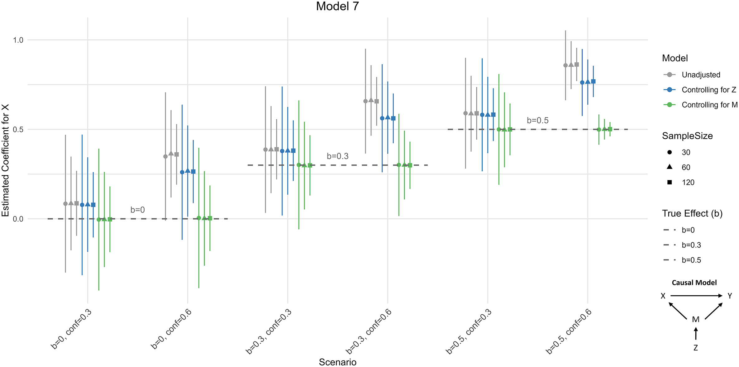
Recommendations for Cross-Cultural Researchers
Given all of the above, what recommendations would we suggest for researchers moving ahead? First, examine if the third variable Z, be it shared ancestry or a confound of some sort, influences Y, the outcome of interest. If there is no association between Z and Y, then one is most likely dealing with Models 3-5, where controlling for Z is either neutral, or it harms the precision of estimates of the X-Y relationship, potentially leading to false negative or otherwise biased conclusions. In such situations, controlling for Z is not recommended, and we would encourage researchers not to do so, and not to recommend doing so (as reviewers).
If there is an association between Z and Y, then one might be dealing with Model 1 or 2. Here, controlling for Z can be useful, as it can correct for bias or improve model estimates. But again, we stress the importance of specifying one’s theoretical causal model. Because without a causal model, Model 1 (where Z is a confounder) is statistically indistinguishable from Model 6 (where Z is a collider). As outlined earlier, if X and Y in fact cause Z (rather than being caused by it), controlling for Z can inflate the estimated effect of X on Y, leading to false discoveries.
Conclusion
In sum, this article argues that while often valuable, controlling for third variables, including recommended controls for geographical and linguistic distances in tackling the problem of non-independence (e.g., Claessens et al., 2023) overlooks both important practical and theoretical considerations when doing cross-cultural research. Solving the problem of non-independence of nations begins with specifying the causal model and target estimand. Confounding becomes a concern only when an omitted variable is a cause of both the predictor and outcome of interest. If it is correlated solely with the predictor, controlling for that variable may be unnecessary and it could cause inefficiency. While well-intended, controlling for background factors like spatial distance and linguistic similarity may even backfire by introducing bias in certain causal models, making it inappropriate as the default strategy. Highlighting this risk is important, as overlooking it could inadvertently lead to potentially creating new issues while seeking to mitigate one. Thus, inspired by Claessens et al. (2023), cross-cultural research must venture into further methodological refinement with an enhanced causal inference mindset.
Supplemental Material
Supplemental Material - Non-Independence of Nations: Revisiting a Centuries-Old Methodological Challenge
Supplemental Material for Non-Independence of Nations: Revisiting a Centuries-Old Methodological Challenge by Plamen Akaliyski and Oliver Sng in Cross-Cultural Research.
Footnotes
Acknowledgements
We thank Quentin Atkinson, Scott Claessens, Stefan Gehrig, Ronald Fischer, Agner Fog, Joshua Conrad Jackson, Mohsen Joshanloo, Thanos Kyritsis, Jackson Lu, Michael Minkov, Boris Sokolov, and Christian Welzel for useful feedback.

Funding
The author(s) disclosed receipt of the following financial support for the research, authorship, and/or publication of this article: The research of the first author was partly supported by the Lingnan University Research Seed Fund (103645).
Declaration of Conflicting Interests
The authors declared no potential conflicts of interest with respect to the research, authorship, and/or publication of this article.
Supplemental Material
Supplemental material for this article is available online.
Notes
Author Biographies
References
Supplementary Material
Please find the following supplemental material available below.
For Open Access articles published under a Creative Commons License, all supplemental material carries the same license as the article it is associated with.
For non-Open Access articles published, all supplemental material carries a non-exclusive license, and permission requests for re-use of supplemental material or any part of supplemental material shall be sent directly to the copyright owner as specified in the copyright notice associated with the article.
