Bifactor Model Is Not the Best-Fitting Model for Self-Esteem: Investigation With a Novel Technique

Abstract

In the measurement of self-esteem, previous research assumes that all respondents are qualitatively similar. The assumption has not been adequately tested. The current study examines its validity using factor mixture modeling. Results reveal two qualitatively distinct classes: the first provides more consistent responses to positive self-esteem items than the second. The correlations between positive and negative self-esteem suggest that self-esteem is essentially unidimensional in the first class but bidimensional in the second. Furthermore, those with high self-esteem are more likely to belong to the first class; those with low self-esteem are more likely to belong to the second class. The observed dimensionality of self-esteem depends on a person’s level on the trait. Finally, we found that the two-class solution fits the data much better than a simple one-class, two-factor solution or a bifactor solution. Psychometric researchers should no longer ignore the possible existence of qualitatively distinct groups in an underlying population. We include Mplus syntax together with a detailed explanation for researchers to conduct similar investigations on constructs of interest.

Keywords

factor mixture modeling reverse-keyed items self-esteem

Researchers often debate whether regular-keyed items and reverse-keyed items measure the same construct. When regular- and reverse-keyed items are subjected to factor analysis, the usual result is that they load on separate factors. For example, in the case of self-esteem, regular-keyed items (positive self-esteem) and reverse-keyed items (negative self-esteem) tend to form two separate factors (Motl & DiStefano, 2002; Shahani et al., 1990). Some researchers take this to mean that positive and negative self-esteem are distinct constructs (Huang & Dong, 2012; Owens, 1993; Shahani et al., 1990), whereas others believe that the result is an artifact due to regular- and reverse-keyed items not being fully compatible with one another (Carmines & Zeller, 1979; Greenberger et al., 2003; Schmitt & Allik, 2005). As suggested by Campbell and Fiske (1959) in a classic article, using distinct means (in this case, items with opposite keying direction) to measure the same construct is unlikely to yield a perfect correlation.

Research regarding the dimensionality of self-esteem may inform clinical practice. If self-esteem is unidimensional, then psychotherapists do not need to attend to raising positive self-esteem and lowering negative self-esteem. If self-esteem is multidimensional, psychotherapists need to attend to both positive and negative aspects. Therefore, the dimensionality of self-esteem has both theoretical and practical implications.

To investigate self-esteem, researchers often construct a model in which a general factor loads on all self-esteem items, and two specific factors load on positive and negative items separately (Tomás & Oliver, 1999). This model, commonly known as the bifactor model, usually fits the data significantly better than either the one- or the two-factor model. Nevertheless, the meaning of the specific factors is something of a mystery. Despite decades of research, surprisingly little progress has been made (Kam, 2018b), and it is uncertain whether this question will ever be fully answered.

To date, self-esteem researchers have assumed that all participants come from the same underlying population. This is known as the assumption of population homogeneity (Lubke & Muthén, 2005): only one model is needed to capture response variance from all participants. Researchers who make this assumption do not necessarily state it explicitly.

The current study examines the assumption of population homogeneity in the measurement of self-esteem. To do so, we will use a fairly new statistical technique—factor mixture modeling (FMM; Lubke & Muthén, 2005)—which has been used previously to evaluate population homogeneity in the measurement of job satisfaction (Kam & Fan, 2018) and optimism (Kam, 2020).

First we provide a brief history of the dimensionality debate concerning self-esteem, elaborating on the common criticisms of the bifactor model in such work. Then, we will discuss the assumption of population homogeneity in previous research and explain why the assumption is shaky. We then suggest an alternative modeling technique to explain self-esteem data. Finally, we report an empirical study that demonstrates the superiority of this method.

Self-Esteem Dimensionality Research and Problems With the Bifactor Model

Self-esteem is defined as participants’ positive or negative global evaluation of self (Rosenberg, 1965). The construct has been a very popular research subject. The most popular scale of self-esteem was developed by Rosenberg (1965). It consists of 10 items, half of which are regular-keyed items (e.g., “On the whole, I am satisfied with myself”) and half of which are reverse-keyed items (e.g., “I feel I do not have much to be proud of”). The construct was initially conceptualized as a unidimensional, bipolar construct, measuring positive self-esteem (or positive self-evaluation) on one pole and negative self-esteem (negative self-evaluation) on the other. However, regular-keyed (positive) items and reverse-keyed (negative) items often loaded on two correlated but separate factors (see Figure 1a; Bachman & O’Malley, 1986; Carmines & Zeller, 1979; Goldsmith, 1986).

Figure 1.

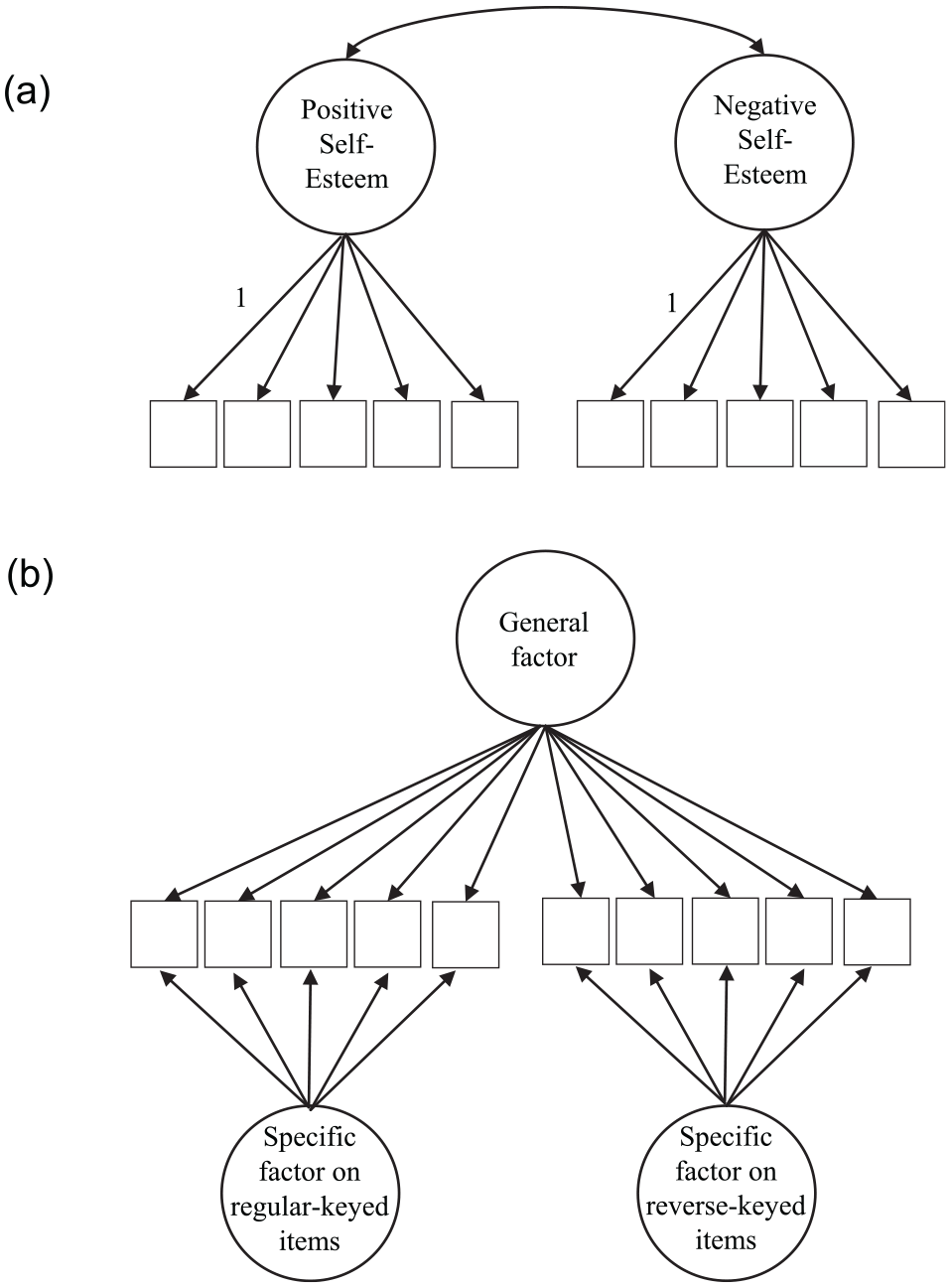
An example of (a) a one-class, two correlated factors model and (b) a bifactor model.

Goldsmith (1986), for example, found a two-factor solution; he also showed that the two factors have slightly different correlations with external variables. Based on these findings, he argued that positive and negative self-esteem have slightly different meanings. Although Carmines and Zeller (1979) also found a two-factor solution, they argued that it was simply a methodological artifact due to contamination by participants’ response set. Marsh (1996) showed that the two-factor solution was at least partly due to participants’ low verbal ability and young age. Greenberger et al. (2003) showed that positive and negative self-esteem correlate similarly across a wide variety of external variables, with the exception of depressive symptoms, which understandably correlate more strongly with negative self-esteem. Overall, most factor analytic research has preferred the two-factor solution, but researchers have widely conflicting explanations for the finding.

Subsequently, using techniques originated in the multitrait–multimethod literature (Campbell & Fiske, 1959), researchers examined the common variance among all self-esteem items and the unique variance specific to keying direction (Motl & DiStefano, 2002; Tomás & Oliver, 1999). This type of model is commonly known as the bifactor model (Figure 1b). Quilty et al. (2006) found that in the bifactor model, the specific factor variance due to keying direction was correlated with avoidance motivation, conscientiousness, and emotional stability. Lindwall et al. (2012) found that the unique variance correlated with depression. DiStefano and Motl (2009) found that it correlated with the fun-seeking subscale in the behavioral activation system, and speculated that it may be predicted by personality characteristics. Marsh et al. (2010) found that specific factor variance was stable over time, but reasons for this stability are unknown. In short, the exact nature of the specific factor variance associated with keying direction is still uncertain.

Some methodologists have criticized the use of bifactor models to explain the factor structure of constructs such as self-esteem (Bonifay et al., 2017). These critics argue that just because a bifactor model has a superior fit does not necessarily mean that the underlying structure of the construct is bifactorial (Bonifay et al., 2017). In their simulation, Bonifay and Cai (2017) demonstrated that a bifactor model is able to accommodate many possible data patterns, even when the true model was not bifactorial. In other words, the bifactor model tends to overfit data.

In their analysis of a large set of actual self-esteem data, Reise et al. (2016) found that many participants fit well in a bifactor model even though they made many implausible and inconsistent responses. Specifically, these participants made inconsistent responses to items with the same keying direction (e.g., agreeing with some regular-keyed items but disagreeing with other regular-keyed items). In contrast, participants who fit well in a unidimensional model tended to provide consistent responses. Based on these results, the researchers argued that self-esteem is largely unidimensional for most participants; the previous finding of bidimensionality was simply the result of improbable and inconsistent responding by some participants. As a result of these latest empirical studies, methodologists caution applied researchers to consider other factors—not just model fit alone—when considering construct dimensionality (Bonifay & Cai, 2017). A construct’s true underlying structure is not necessarily captured by the best-fitting model.

Bifactor models in general are methodologically controversial not only because they can accommodate improbable responses but also because it is difficult to interpret the substantive meaning of the factor scores associated with these models (Reise et al., 2016). As mentioned, a bifactor model usually has a general factor that loads on all items and a specific factor that loads mostly on reverse-keyed items. As Reise et al. (2016) showed, the specific factor can be caused by improbable or invalid responses. They caution that even if these improbable or invalid responses can be reliably identified from all participants, there is currently no method to turn the factor scores associated with those problematic responses into valid scores. Consequently, the meaning of the factor scores is unknown.

For decades, research has examined the nature of the specific factor by correlating it with other variables (such as social desirability and personality factors; e.g., Kam & Meyer, 2015; Quilty et al., 2006)—but we are still without a definitive conclusion. Kam (2018b) found that specific factors across multiple scales do not necessarily correlate strongly with one another, implying that the nature of the specific factor may be scale-dependent and may not have substantive meaning. As a result, methodologists have suggested that the bifactor model be used only to compare the relative contributions of the general factor and the specific factor. If the general factor explains most of the total factor variance (the sum of the general factor variance and the specific factor variance), they suggest that the construct can be regarded as “essentially unidimensional” (Rodriguez et al., 2016). It has been suggested that no substantive interpretation of the keying direction factor in a bifactor model should be made.

There is one final criticism of the bifactor model to be made, but before elaborating, we will first explain the meaning of population heterogeneity and the risk that a bifactor model might disguise it.

Population Heterogeneity and Factor Mixture Modeling

Recent research by Raykov et al. (2019) has shown that a bifactor model may disguise population heterogeneity in a data set. Most research assumes that samples within a population are qualitatively homogeneous, and any deviation from an estimated parameter value is due to random errors. Therefore, only one set of parameter values is sufficient to describe all participants in a sample. A typical example would be a simple unidimensional model or a bifactor model. All participants are assumed to be qualitatively similar. However, as argued by some researchers (e.g., Kam & Fan, 2018), there is usually no strong reason to assume population homogeneity.

The opposite of population homogeneity is population heterogeneity, which requires more than one set of parameter values to describe a population. Figure 2 shows a population heterogeneity model for self-esteem. In such a model, there are subgroups within the population, each of which has a unique set of parameter values. Therefore, multiple sets of parameter values are required to adequately describe the population. Although the term population heterogeneity is rarely heard, its examples are abundant in social scientific research. For example, in a typical multigroup comparison between two cultural groups in a confirmatory factor analysis (CFA) model, each group is allowed to have its own set of parameter values. Differences in these parameter values between the cultural groups can be compared. Thus, cultural groups can differ in item factor loadings, factor means, item intercepts, and other parameters.

Figure 2.

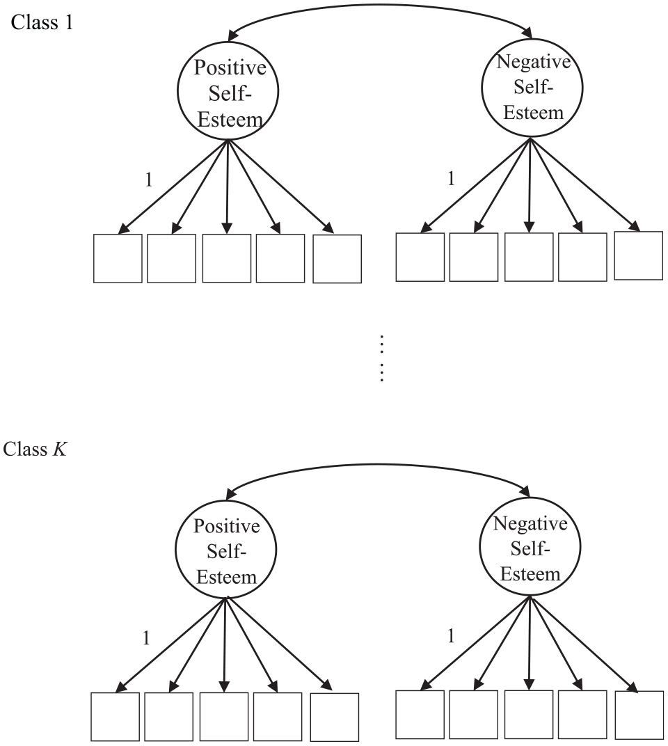
A factor mixture model in the current study.

Of course, in such multigroup CFA models, group membership is known in advance. Recent advances in methodology allow the possibility of analysis even when group membership is unknown before data analysis. FMM can detect previously invisible population heterogeneity, and thereby discover subpopulations (also called classes) within a data set (Lubke & Muthén, 2005). The number and nature of subpopulations is an unknown, latent variable. Therefore, using FMM, researchers are now able to classify participants into different subpopulations.

FMM can be conceptualized as a combination of two popular approaches in statistical analysis: the modeling method and the taxonomic method (Lubke & Muthén, 2005). Modeling methods, such as CFA, give researchers flexibility to build statistical models that specify the relationships among observed indicators (such as survey items). Each indicator may load on any latent factor, and the latent factors are allowed to correlate or covary with each other. Taxonomic methods, such as cluster analysis, investigate the possibility that participants belong to several qualitatively distinct groups. Each member of a group shares characteristics, but individuals from different groups do not. An example is major depressive disorder. Individuals with major depression have characteristics in common, such as depressive mood and loss of interest or pleasure for two weeks or longer. Individuals without depression do not possess these characteristics. However, traditional taxonomic methods do not allow statistical modeling in each group, whereas FMM does. FMM estimates the probability that a given participant belongs to a particular group. Participants are assigned to their most likely group. Participants in the same group are assumed to share a set of parameter values.

Recently, Raykov et al. (2019) simulated a factor analytic model that consists of several subpopulations, where each subpopulation had its own set of parameter values. Even though each subpopulation was a qualitatively distinct data set, a single bifactor model fit the combined data sets well. The lesson is that a bifactor model has the potential to disguise unobserved population heterogeneity. Methodologists therefore advise applied researchers to routinely apply appropriate procedures to examine the possibility of population heterogeneity, rather than blindly applying a bifactor model, as in most previous studies.

Using FMM to Uncover Population Heterogeneity

Kam and Fan (2018) recently applied the methodology of Litson et al. (2017) to study possible population heterogeneity in the measurement of job satisfaction. Notwithstanding previous research, which assumes population homogeneity, Kam and Fan (2018) discovered the existence of two subpopulations. Subsequent analysis showed that the first class features consistent responding and the second-class features inconsistent responding, such as agreeing with some reverse-keyed items but disagreeing with other reverse-keyed items even though the items are supposed to share similar content. These results suggested that a substantial number of respondents have trouble answering the scale items. Most important, the correlation between job satisfaction and job dissatisfaction was strong enough to conclude that the construct is essentially unidimensional—but only for the first class of respondents. Previous research suggesting a distinction between job satisfaction and dissatisfaction (Credé et al., 2009) can thus be considered an artifact caused by inconsistent responding.

Kam (2018a) used the procedure of Kam and Fan (2018) to investigate the possibility of population heterogeneity in the measurement of dispositional optimism. A similar result was found: the construct can be considered essentially unidimensional, but only for the response-consistent class. Overall, the results suggest that inconsistent responding can distort the factor structure of a construct, at least for the measurement of job satisfaction and optimism.

The current study examines possible population heterogeneity in the measurement of self-esteem. As noted earlier, the dimensionality of self-esteem is often the subject of study, but most research on the topic assumes population homogeneity. In situations where population heterogeneity exists, the empirical conclusions of these studies could be severely compromised due to the unexamined assumption of homogeneity. If there are multiple classes of individuals in terms of self-esteem, it is possible that positive and negative self-esteem correlate most strongly for one class or level of self-esteem, but correlate less strongly for other classes, which have different levels of self-esteem.

We employed the procedure described by Kam and Fan (2018) and Litson et al. (2017) to examine potential population heterogeneity and to discover possible novel insights regarding the dimensionality of self-esteem. In a population heterogeneity model (Figure 2), positive and negative self-esteem load on two separate factors, which are allowed to covary. The analytic process estimates the extent to which item covariation is due to class membership or latent factors within a class. Each class is allowed to have a separate set of parameter values. Rosenberg’s Self-Esteem Scale (RSES; Rosenberg, 1965) was used. The RSES is a very popular self-esteem measure across various age groups, and its validity has been well documented (Blascovich & Tomaka, 1993; Bleidorn et al., 2016). FMM will be employed to model a large set of self-esteem data, as described in the Data Analysis section below.

Method

Data came from a free and open website (https://openpsychometrics.org/_rawdata/), where numerous personality raw data are stored and freely downloaded. The current data set consists of 47,929 participants who completed an online self-esteem survey around the globe. According to the website, participants’ identity was anonymous and was not tracked. Participation was voluntary; the only data included had participants’ consent for research purposes.

Rosenberg Self-Esteem Scale

Participants completed the 10-item RSES (Rosenberg, 1965) in English. Half of the items were regular-keyed and half were reverse-keyed. Participants answered each item on a 4-point Likert-type scale (1 = strongly disagree; 4 = strongly agree). Cronbach’s alpha was high (.91).

Data Analysis

Given the type of data collection, it is necessary to control for careless responding (Kam & Meyer, 2015). To detect careless responding, methodologists suggest that we use several indices with loose cutoff criteria, and include only respondents who pass all the cutoffs (i.e., multiple hurdles approach). In this way, false positives can be minimized (Goldammer et al., 2020). The indices in the current study involve Mahalanobis distance (MD), long string, and the person-fit index (standardized log-likelihood, or l_z). MD detects response patterns that deviate from the multivariate normal (Hong et al., 2019). The long-string approach detects responses to items of diverse content that are suspiciously similar. The standardized log-likelihood index detects deviations from the unidimensional item response theory model (Hong, Steedle, & Cheng, 2019).

In the case of self-esteem, it is at least reasonable to assume that regular-keyed items measure a common construct, and therefore responses to them should be very consistent. Therefore, we calculated MD and the standardized log-likelihood index based on the five regular-keyed self-esteem items; respondents were excluded who deviated significantly at α = .05 (i.e., MD > 18.31 and l_z < −1.64). For long string, out of 10 self-esteem items, the longest string of items with the same keying direction was three. To minimize false positive cases, we excluded respondents who made more than four consecutive identical responses. The final sample included 40,940 respondents (i.e., 14.6% were excluded).

After exclusion of careless respondents, the data were analyzed using a procedure similar to that of Kam (2018a), Kam and Fan (2018), and Litson et al. (2017). We employed the Mplus program version 7.11 (Muthén & Muthén, 2012) to conduct FMM, along with robust maximum likelihood estimator to account for nonnormality in the data. We first set up a two-factor model, with positive self-esteem items loaded on one factor and negative items loaded on another factor. The two latent factors were allowed to covary, and thus their correlation could be examined. This is a basic (one-class) CFA model, because it is assumed that the same model (with the same parameters) applies to all participants. It features population homogeneity, which, as noted, is a characteristic commonly assumed in previous construct dimensionality research.

Next, we examined the possibility of population heterogeneity by setting up a two-class model. Participants in each class were allowed to have distinct parameter values (e.g., different factor loadings, factor covariance/correlation), but participants within the same class were assumed to be qualitatively similar, and thus they had identical model parameters. We continued the process by setting up a three-class model, four-class model, and so on, until the model fit deteriorated. Finally, we chose the best among these various models. If any of the multiple-class models fit better than the one-class model, the assumption of population homogeneity in previous construct dimensionality studies would be undermined.

Model fit among various multiple-class models can be compared using the Akaike information criterion (AIC), the Bayesian information criterion (BIC), and sample-size adjusted BIC (SABIC). A model with lower values indicates better fit. Among these three indices, BIC has received the most support in model comparisons. However, as noted in the Introduction, excessive reliance on model fit indices is likely to result in overextraction of classes, particularly when the number of participants is large (as in the current case). Therefore, we should also consider the interpretability of any given solution, and choose a model that makes the most sense. Finally, entropy does not indicate the accuracy of a solution, but a higher entropy value is preferred because it indicates greater classification accuracy.

After identification of the best class, we will follow the recommendation of Kam and Fan (2018) and compute an “inconsistency index”—the difference between the maximum and minimum response value for regular-keyed items (positive self-esteem). We calculate the same index for reverse-keyed items (negative self-esteem). A low value is preferred, because participants are supposed to provide similar responses to items with similar content. In addition, research suggests that some participants may not give logically consistent answers to positive and negative self-esteem items (e.g., they may agree with both positive and negative items; Campbell, 1990; Reise et al., 2016). Therefore, we will also examine the difference between positive and negative self-esteem scores for each class. Given the extremely large sample size, all significance levels in the current study are set at .001 to avoid statistically trivial results. Finally, although a bifactor model is difficult to interpret, we will compare the model fit of our final solution with a bifactor model.

Results

Investigation of Population Heterogeneity

We first set up a (one-class) two-factor model. The model fit was generally adequate, χ² = 12088.91, degrees of freedom = 34, p < .001, Tucker–Lewis index = .93, comparative fit index = .95, root mean square error of approximation = .09, standardized root mean square residual = .03. The correlation between positive and negative self-esteem items was high (−.90), but significantly different from 1, p < .001, meaning that a one-factor model would fit the data significantly worse.¹ Then, we examined the possibility of a multiple-class model. We requested a two-class solution, a three-class solution, and so on. Model fit results are shown in Table 1.

Table 1.

Fit Indices.

	AIC	BIC	SABIC	Entropy
One-class (two correlated factors)	842823.81	843091.03	842992.51	—
Two-class configural invariance	821343.14	821886.20	821685.98	.75
Two-class factor loading invariance (all items)	823190.22	823664.31	823489.52	.75
Two-class (with factor loading invariance for pse items only)	822060.75	822569.32	822381.82	.75
Two-class (with factor loading invariance for nse items only)	822771.45	823280.02	823092.52	.74
Three-class	(nonconvergent)
Four-class	(nonconvergent)

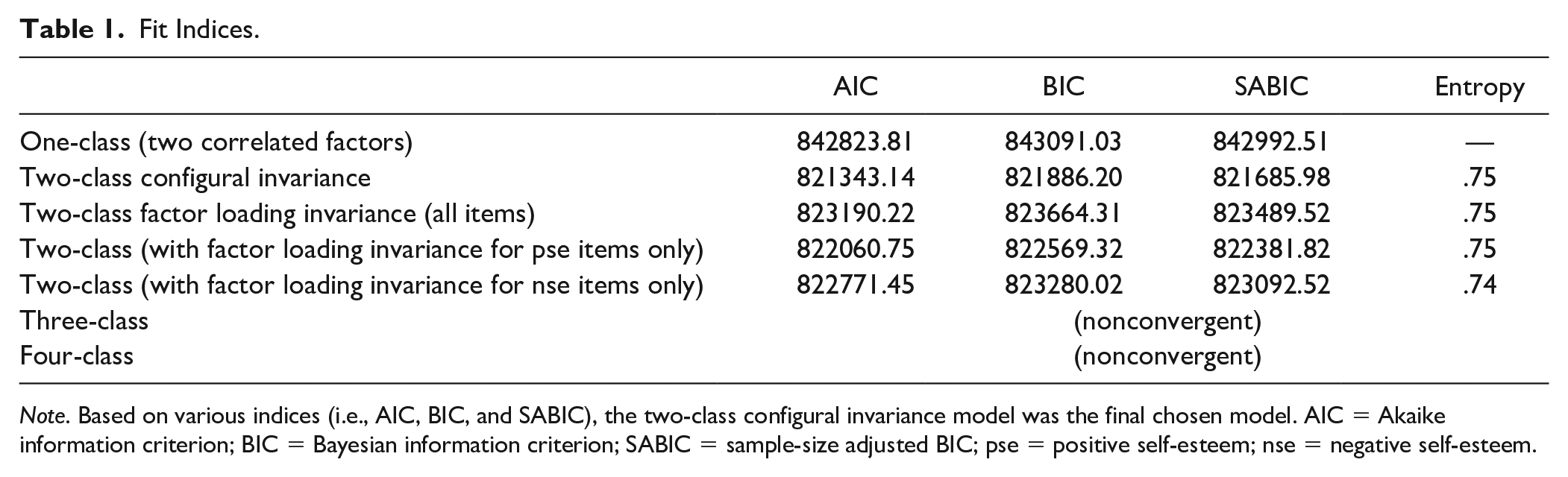
Note. Based on various indices (i.e., AIC, BIC, and SABIC), the two-class configural invariance model was the final chosen model. AIC = Akaike information criterion; BIC = Bayesian information criterion; SABIC = sample-size adjusted BIC; pse = positive self-esteem; nse = negative self-esteem.

The two-class, configural invariance solution separated participants into two groups: Class 1 had a slightly larger percentage of respondents (50.27%) than Class 2 (49.73%). We then tested a model in which item factor loadings were constrained to be identical between the two classes (i.e., factor loading invariance model). Other parameters (e.g., factor variance, item intercept) remained to be freely estimated. This factor loading invariance model was not supported, because all factor loading invariance models increased AIC, BIC, and SABIC values compared with the configural invariance model (Table 1). Therefore, a configural model without factor loading invariance is preferred. The factor correlation was −.80 in Class 1 and −.64 in Class 2. The consensus is that two factors are considered to be the same (i.e., unidimensional) if they correlate at |.80| or above. The difference between positive and negative self-esteem scores was smaller in Class 1 as compared with Class 2 (Ms = 0.42 vs. 0.71), p < .001.

A model with three or more classes could not converge to a proper solution. Among the remaining classes, the fit indices indicated that a two-class model with configural invariance had the lowest AIC, BIC, and SABIC values, and thus we conclude that this is the final model (Figure 3).

Figure 3.

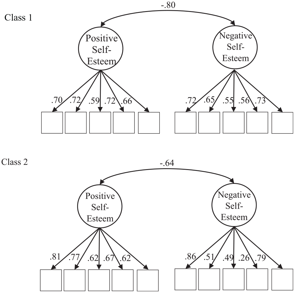
Final model in the current study.

Dimensionality of the Two Classes

We then checked the dimensionality of self-esteem in each class. Further analyses of the correlations between positive and negative self-esteem suggested that the correlation in all two classes differs from 1, because its 95% confidence interval does not include 1 (Table 2). Therefore, self-esteem is not a unidimensional construct in any of these classes. We then checked for essential unidimensionality in the two classes. It is unrealistic to expect strict undimensionality for constructs measured by different keying directions (here, regular- vs. reverse-keyed items). Therefore, researchers (Gu et al., 2017; Rodriguez et al., 2016) recommend the calculation of explained common variance. To do so, we extracted class membership and set up a bifactor model for each class, with all items loading on a general factor and reverse-keyed items (negative self-esteem items) loading on a specific factor. The general factor and the specific factor are constrained to be orthogonal to each other. If the general factor explains a large amount of variance in any class, then the construct can be deemed essentially unidimensional in that class. Explained common variance was found to be .81 and .74 in the first and the second class, respectively. Therefore, the general factor explained more variance in the first class than the second. Given that the factor correlation between positive and negative self-esteem was −.80 and −.64 in Class 1 and Class 2, respectively, self-esteem is likely to be essentially unidimensional in Class 1 and bidimensional in Class 2.

Table 2.

Model Parameters of the One-Class Solution and the Two-Class Solution.

	One-class	Two-class
	One-class	Class 1	Class 2
Percentage of participants	100	50.49	49.51
Standardized loading
pse1. (a person of worth)	.83 (.002) [.82, .83]	.70 (.006) [.69, .71]	.81 (.005) [.80, .82]
pse2. (having a number of good qualities)	.79 (.002) [.78, .79]	.72 (.007) [.71, .73]	.77 (.005) [.76, .78]
pse3. (doing things as well as others)	.71 (.003) [.70, .71]	.59 (.007) [.58, .60]	.62 (.007) [.61, .63]
pse4. (taking a positive attitude)	.86 (.002) [.85, .86]	.72 (.008) [.70, .73]	.67 (.010) [.65, .69]
pse5. (satisfied with oneself)	.83 (.002) [.83, .84]	.66 (.008) [.64, .67]	.62 (.010) [.60, .64]
nse1. (at times no good)	.84 (.002) [.83, .84]	.72 (.007) [.70, .73]	.86 (.007) [.85, .87]
nse2. (feeling like failure)	.80 (.003) [.79, .81]	.65 (.008) [.63, .66]	.51 (.016) [.48, .54]
nse3. (not feeling proud)	.76 (.003) [.75, .76]	.55 (.010) [.53, .57]	.49 (.016) [.45, .52]
nse4. (wish more respect for oneself)	.60 (.004) [.59, .61]	.56 (.008) [.55, .58]	.26 (.015) [.24, .29]
nse5. (thinking oneself as being no good)	.79 (.003) [.78, .79]	.73 (.007) [.71, .74]	.79 (.010) [.77, .81]
Factor correlation	−.90 [−.89, −.90]	−.80 [−.78, −.82]	−.64 [−.60, −.67]
Factor means
pse score	3.03	3.52	2.53
nse score (after reversal)	2.54	3.09	1.83
Factor variance
pse score	0.52	0.14	0.49
nse score	0.83	0.41	0.58

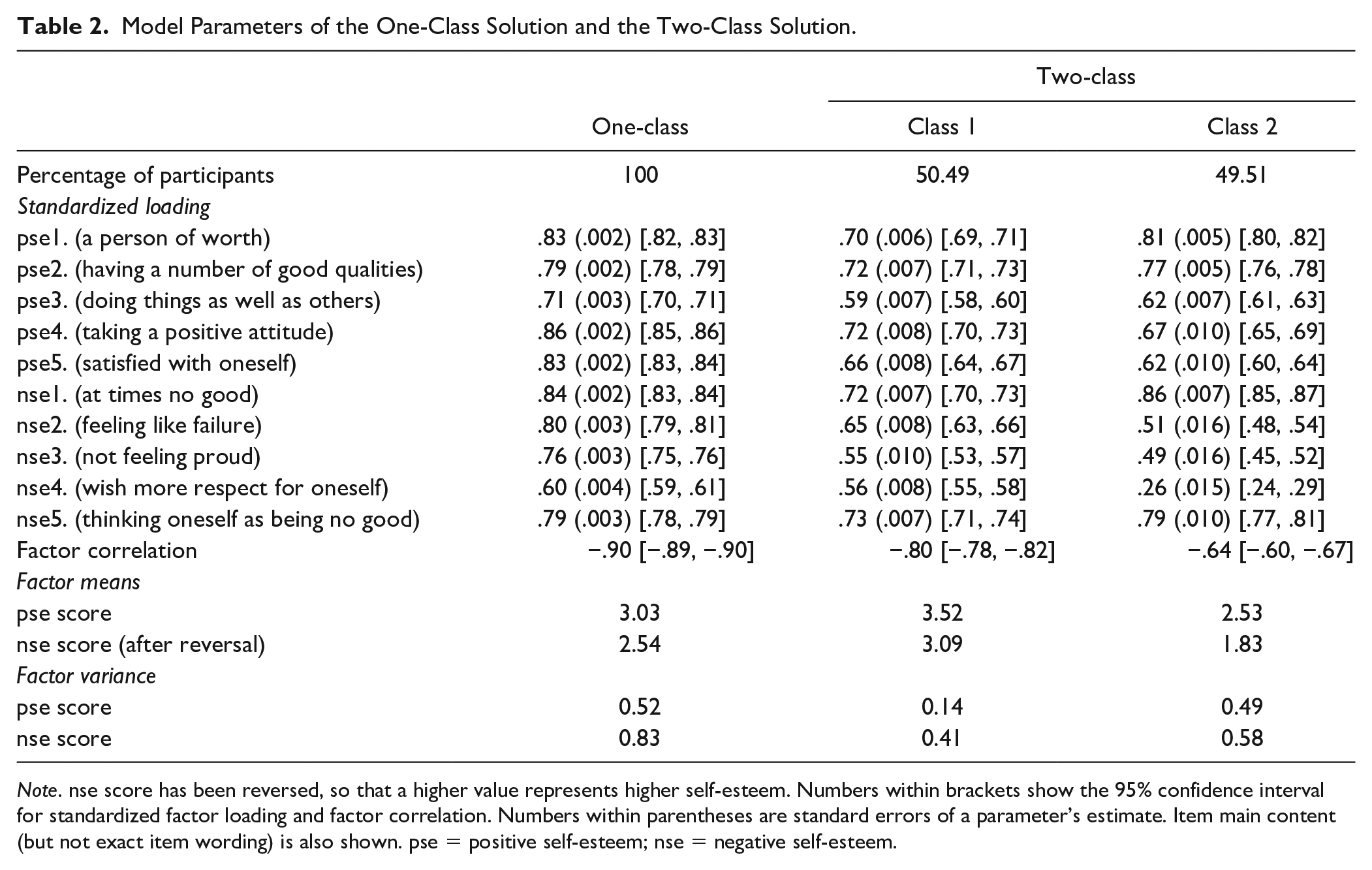
Note. nse score has been reversed, so that a higher value represents higher self-esteem. Numbers within brackets show the 95% confidence interval for standardized factor loading and factor correlation. Numbers within parentheses are standard errors of a parameter’s estimate. Item main content (but not exact item wording) is also shown. pse = positive self-esteem; nse = negative self-esteem.

Characteristics That Differentiate the Two Classes

We further examined mean differences between the two classes on other variables using the procedure of Vermunt (2010). Results showed that the inconsistency index for negative self-esteem was similar in Class 1 and Class 2 (Ms = 1.35 vs. 1.33, Cohen’s d = 0.03), but for positive self-esteem, it was significantly smaller in Class 1 than Class 2 (Ms = 0.81 vs. 1.42, Cohen’s d = 1.00, p < .001). In Class 1, the inconsistency index was higher for negative than positive self-esteem (Ms = 1.35 vs. 0.81, Cohen’s d = 0.77, p < .001); in Class 2, it was slightly higher for positive than negative self-esteem (Ms = 1.42 vs. 1.33, Cohen’s d = 0.13, p < .001). In addition, overall self-esteem was significantly larger in Class 1 than Class 2 (Ms = 3.22 vs. 2.09, Cohen’s d = 2.42, p < .001; see Table 3). According to Cohen (1988), the effect size is small for d = 0.20, medium for d = 0.50, and large for d = 0.80. Therefore, the effect sizes are considered large for differences in (a) positive self-esteem inconsistency and (b) overall self-esteem between classes.

Table 3.

Inconsistency Indices and Overall Self-Esteem Scores in the One-Class Solution and the Two-Class Solution.

	One-class	Two-class
	One-class	Class 1	Class 2	Effect size (d)
pse inconsistent index	1.11	0.81_a	1.42_b	1.00
nse inconsistent index	1.34	1.35_a	1.33_b	0.03
Overall self-esteem score	2.66	3.22_a	2.09_b	2.42

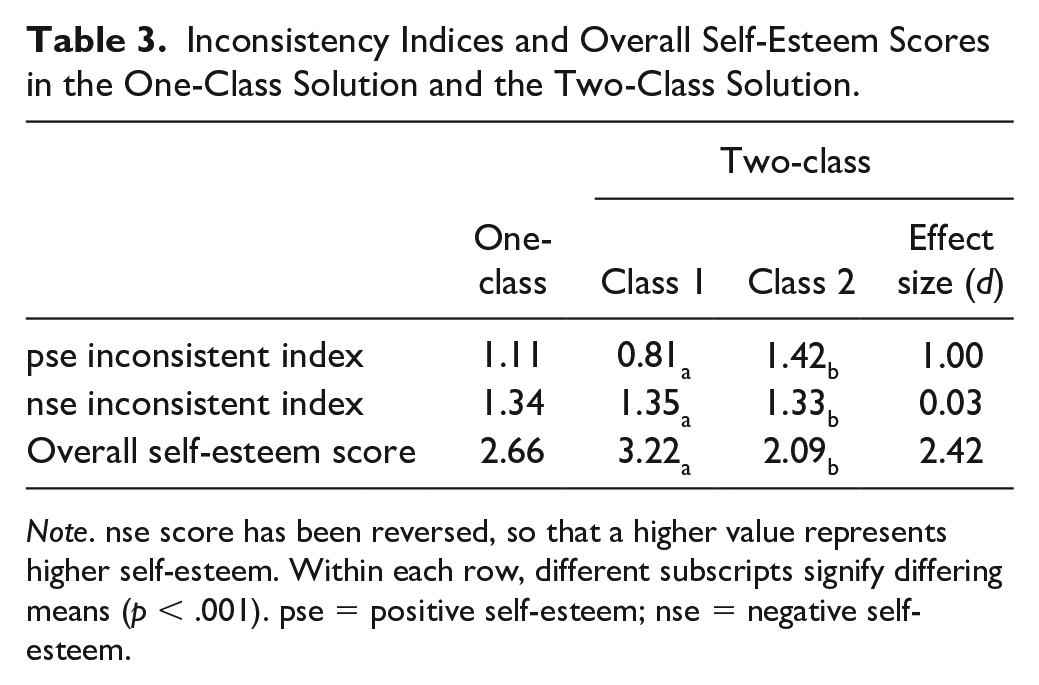
Note. nse score has been reversed, so that a higher value represents higher self-esteem. Within each row, different subscripts signify differing means (p < .001). pse = positive self-esteem; nse = negative self-esteem.

Finally, we attempted to examine which variables significantly contributed to the separation of classes. Using the three-step procedure of Vermunt (2010), we entered five variables—two inconsistency indices, overall self-esteem, gender (with female coded as the higher value), and age—to predict class membership. (Positive and negative self-esteem were excluded because they correlate so strongly with overall self-esteem that multicollinearity is the result.)

Unstandardized results from a logistic regression analysis, using Class 2 as the reference class, suggest that all predictors significantly predict class membership: inconsistency_pse: B = −3.55, standard error (SE) = 0.08, t = 43.12, p < .001, odds ratio (OR) = 0.03; inconsistency_nse: B = 0.36, SE = 0.05, t = −7.28, p < .001, OR = 1.44; overall self-esteem: B = 8.37, SE = 0.14, t = 60.23, p < .001, OR = 4315.64; gender: B = 0.24, SE = 0.07, t = −3.57, p < .001, OR = 1.27; and age: B = −0.01, SE = 0.003, t = 4.77, p < .001, OR = 0.99. To assist comparisons between the various predictors, we standardized all predictors and put them in the logistic regression analysis (except gender, which is a categorical predictor). The regression coefficients remained large for the following two variables: inconsistency_pse: B = −2.43, p < .001, OR = 0.09; overall self-esteem: B = 6.13, p < .001, OR = 459.44, suggesting that both are important. In comparison, the regression coefficients appeared to be much smaller for age (B = −0.17, p < .001, OR = 0.84) and inconsistency_nse (B = 0.30, p < .001, OR = 1.35). With the reference group as Class 2, participants with higher overall self-esteem and lower response inconsistency to positive items are more likely to belong to Class 1.

Bivariate correlational analyses (Table 4) showed that (a) age had almost no association with response inconsistency (|r|s ≤ .05); (b) inconsistency indexes to positive and negative items were only weakly correlated (r = .14), and (c) self-esteem was negatively associated with inconsistent responding for positive (r = −.32) but not for negative items (r = .001). Those with high self-esteem are more likely to provide consistent responses to positive self-esteem items. As implied by the low correlation between inconsistency_pse and overall self-esteem, they seemed to have uniquely contributed to the separation of the two classes, as shown in our previous logistic regression analysis.

Table 4.

Correlations.

	1.	2.	3.
1. Age
2. Overall self-esteem level	.25***
3. Inconsistency_pse	−.05***	−.32***
4. Inconsistency_nse	−.04***	.001	.14***

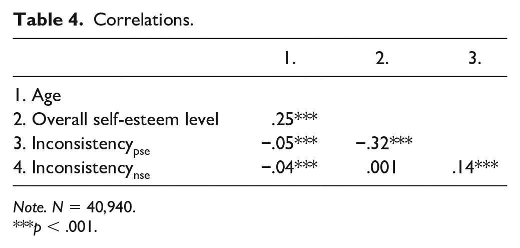
Note. N = 40,940.

***

p < .001.

Probability of the Two-Class Solution Versus the One-Class Solution

BIC values suggested that the most tenable model of self-esteem was the two-class configural invariance model. However, previous research often assumed a one-class solution in which positive and negative self-esteem is correlated (Figure 1a), so it may be useful to explicitly compare the one-class (two correlated factors) solution with the two-class solution. We used a Bayesian model selection method (Wu et al., 2019) to compare the two-class configural invariance solution with the one-class solution. According to Wu et al. (2019), one model is at least 1,000 times more likely than another model if the difference in BIC is 14 or more between them. Given that the two-class configural invariance model is much smaller than the one-class model (ΔBIC = 21204.83; Table 1), the former model is much more likely.

Although a (one-class) bifactor model (Figure 1b) is usually theoretically difficult to interpret, it is still worthwhile to examine the extent to which a bifactor model can provide a good fit to our data, as compared with the best two-class model. In a bifactor model, one general factor loads on all self-esteem items and two specific factors load on positive and negative self-esteem items independently. The general factor does not correlate with the specific factors. In one version of the bifactor model, the specific factors are not correlated with each other (i.e., one-class, uncorrelated specific factors model). In another version, the general factor remains uncorrelated with the specific factors but the specific factors are correlated (i.e., one-class, correlated specific factors model). In two other versions, the specific factor loaded only on positive or negative self-esteem items (i.e., bifactor-(S − 1) models; Eid et al., 2017). Results of the analysis are shown in Table 5.

Table 5.

Model Fit of Bifactor Models.

	χ²(df)	p	TLI	CFI	RMSEA	SRMR	AIC	BIC	SABIC
Uncorrelated specific factors	2044.21 (25)	<.001	.98	.99	.04	.01	831508.81	831853.61	831726.49
Correlated specific factors	2069.91 (24)	<.001	.98	.99	.05	.01	831499.52	831852.93	831722.63
One specific factor only (on positive self-esteem items)	9728.76 (30)	<.001	.93	.96	.09	.03	839951.82	840253.52	840142.29
One specific factor only (on negative self-esteem items)	7668.27 (30)	<.001	.95	.97	.08	.02	837616.46	837918.16	837806.93

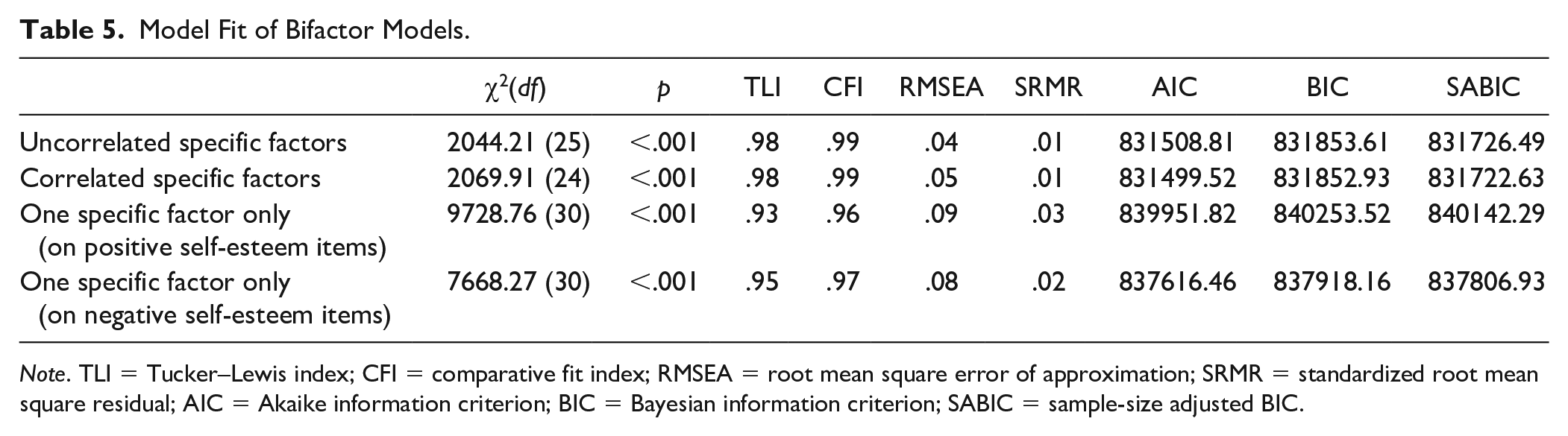
Note. TLI = Tucker–Lewis index; CFI = comparative fit index; RMSEA = root mean square error of approximation; SRMR = standardized root mean square residual; AIC = Akaike information criterion; BIC = Bayesian information criterion; SABIC = sample-size adjusted BIC.

Marsh et al. (2010) found the uncorrelated specific factors model to be the best-fitting among all bifactor models for self-esteem. The current study found that the uncorrelated specific factors model and the correlated specific factors model had similar fit: they shared the lowest BIC values (831853.61 vs. 831852.93) among all bifactor models. However, the best bifactor model still fit worse than the two-class configural invariance model in terms of AIC, BIC, and SABIC. The BIC differences between the two-class configural invariance model and the bifactor models remain huge (ΔBICs ≥ 9966.73), meaning that the two-class configural invariance model was much more likely (Wu et al., 2019). Therefore, the two-class model is strongly preferred.

Discussion

Although the psychometric properties of self-esteem have often been studied, its dimensionality is still a matter of debate. The current study provides several new insights into self-esteem and assessment more generally. First, this study is one of the first to demonstrate that population homogeneity does not hold for the measurement of self-esteem. This in itself suggests a possible reason that many previous studies of the dimensionality of self-esteem data failed to find a single best-fitting model. Second, our analysis showed that participants in Class 1 provided more consistent responses to positive than negative self-esteem items, and for this class of respondents, there is a substantial correlation between positive and negative self-esteem (r = −.80): self-esteem can be considered essentially unidimensional in this class. However, for the other class of participants—the ones who provided inconsistent responses to positive items—self-esteem can be considered two-dimensional. Self-esteem score was higher in Class 1 than Class 2. Both response consistency and overall self-esteem significantly predict class membership. Third, both classes have trouble providing consistent responses to negative self-esteem items, but the difference between positive and negative self-esteem scores was smaller in Class 1 as compared with Class 2. These findings have many implications.

Previous researchers implicitly assumed that all participants come from the same underlying population, and thus one set of parameter values is sufficient to describe all participants. The assumption was convenient, as it allowed researchers to use basic statistical techniques such as CFA to analyze the data. Unfortunately, the tenability of the assumption was seldom tested, which led to much confusion concerning the dimensionality of the construct. The current results reveal the invalidity of the homogeneity assumption: a model with two qualitatively distinct classes fit the data much better than the traditional one-class solution. Furthermore, the two-class model is at least 1,000 times more probable than both the one-class (two-correlated-factors) model and any of the bifactor models. Given the large sample size in our data, the finding that the two-class model is more probable than those other models is unlikely due to chance. Given that previous research mostly assumes a one-class solution for self-esteem, the results and conclusions of these studies are possibly severely compromised. In this respect, the current research demonstrates the usefulness of advanced quantitative techniques for answering questions in psychological assessment (e.g., Marsh et al., 2010). Although these procedures may require substantial investment of time and resources, the payoff, we believe, is worth it, and accordingly urge self-esteem researchers to consider the possibility of population heterogeneity in the measurement of self-esteem.

We found that the dimensionality of a construct is associated with response consistency and level of self-esteem. The participants who had trouble providing consistent responses to positive self-esteem items had a relatively low correlation between positive and negative self-esteem (r = −.64). Positive and negative self-esteem are related but distinct constructs for this group. These respondents have relatively low trait self-esteem. In contrast, the participants who provided consistent responses to positive self-esteem items had a high correlation between positive and negative self-esteem (r = −.80); self-esteem can be regarded as essentially unidimensional for them. These respondents have relatively high trait self-esteem.

If we consider the use of regular- and reverse-keyed items as distinct means to measure a given construct, the correlation between the two means depends on one’s standing on the self-esteem trait. The dependence of factor correlations on a person’s trait level is seldom studied in psychological literature, with some exceptions (Hintz et al., 2019; Litson et al., 2017). To our knowledge, the current study is the first to demonstrate the dependence of factor correlations on a person’s trait level in the measurement of self-esteem. Our finding is noteworthy because a bifactor model assumes no correlation between trait and specific factors, and thus it cannot investigate the interaction between factor correlations and one’s trait level (Hintz et al., 2019).

What could explain the low correlation between positive and negative self-esteem items for participants with low self-esteem? The self-esteem research by Campbell and colleagues is relevant to our discussion. Among participants who rated themselves on personality traits, low self-esteem was associated with lower certainty, lower confidence, and less response extremity (Campbell, 1990). Over a 2-month period, temporal stability of self-ratings was lower for them, and their reaction time to personality items was slower. People with low self-esteem were more likely to provide inconsistent answers to pairs of adjective opposites (e.g., agreeing that they were both timid and bold; Campbell, 1990). Taken together, these studies suggest that low self-esteem is associated with lower clarity of self-concept—knowledge about oneself (Campbell, 1990; Campbell et al., 1996). Compared with those with high self-esteem, low self-esteem individuals are less certain about who they are. Consistent with these findings, the current study discovered distinct response behaviors among participants: low self-esteem participants have more trouble providing consistent responses to positive self-esteem items than high self-esteem participants. This is noteworthy because of the connection between previous social psychological research and the present psychometric research. Response inconsistency on positive self-esteem items results in a lower correlation between positive and negative self-esteem in this class of respondents.

It should be noted that both classes of respondents have trouble providing consistent answers to negative self-esteem items. The value of negative self-esteem items should be evaluated, given the difficulty they cause participants. Previous research (Kam, 2018a) has suggested that respondents may have more trouble admitting possession of negative characteristics than endorsing ownership of positive characteristics. Our finding of inconsistent responding on negative self-esteem items accords with the recommendation from some previous researchers (e.g., Quilty et al., 2006) to exclude them.

Implications for Self-Esteem Dimensionality Research

In previous self-esteem research, a unidimensional model was often compared with a bifactor model. The bifactor model usually featured a general factor representing variance from all items and a specific factor representing variance due to item-keying direction. The discovery of the specific factor is not recent: it was found in very early self-esteem research (e.g., Marsh, 1996). Unfortunately, decades of research have done little to illuminate the specific factor. Although it has been found to correlate with some personality and clinical variables, the correlations tend to be weak. For instance, Tomás et al. (2013) found that trait anxiety weakly predicted the specific factor associated with negative self-esteem (standardized β = −.37). Similarly, they found that the specific factor related to negative self-esteem is negatively predicted by depression (standardized β = −.32) and positively predicted by life satisfaction (standardized β = −.11). None of these relationships was high enough to conclude that negative self-esteem represents anxiety, depression, or life satisfaction. In addition, because correlation does not imply causation, it is impossible to infer any direct relationships between self-esteem and those other variables.

Kam (2018b) showed that the specific factors from various scales do not correlate well with one another, implying no consistent specific factors across scales. Although self-esteem was not included in his study, the specific factors from a close correlate of self-esteem—neuroticism—correlated at .56 with extraversion, but only −.01 with openness to experience. Therefore, the nomological network (Campbell & Fiske, 1959) of specific factors vary substantially across measurement scales. Other research (e.g., Rauch et al., 2007) suggests that specific factors can be the result of social desirability, participants’ tendency to report themselves in an overly positive manner. Again, no consistent correlation between social desirability and specific factors was found by Kam (2018b). For instance, impression management, which is one facet of social desirability, has a moderate relationship with the specific factor from agreeableness (r = −.56, p < .001) and a weak relationship with the specific factor from neuroticism (r = −.15, p < .001), but no relationship with the specific factor from openness (r = .01, ns). The inconsistency of these correlations make it difficult to reach any general conclusions. At one time, it seemed that the ongoing investigation of specific factors had reached a dead end.

Researchers echo this sentiment. Bonifay et al. (2017) explained two common uses of a bifactor model containing a general factor and a specific factor. The first was to understand the amount of variance among measurement items that are captured by the general factor, and they approve of this use as a way to understand the psychometric properties of a measurement scale. The second was to investigate the underlying structure of a construct. Bonifay et al. strongly criticized this use. Analogous to the motto “correlation does not imply causation,” they pointed out that a factor structure that fits the data well does not necessarily imply the latent causal structure of a construct. There may be different processes involved that generate the correlations among the items, and the bifactor structure can camouflage these processes. This caution has been largely underappreciated in the psychometric community. Consistent with this claim, and as pointed out earlier, the bifactor model can overfit by accommodating noisy data, even nonsensical responses (Reise et al., 2016). Simulation investigations have found that the bifactor model can fit the data well even when the true model has a different structure (Murray & Johnson, 2013) or when the data is randomly generated (Bonifay & Cai, 2017).

Consequently, an interesting question is to what extent our findings represent the true structure of a construct. Although recent researchers have questioned the ability of a bifactor model to reflect the true nature of a construct, the same doubt can be applied to a factor mixture model: our results do not preclude the possibility of an unknown model that may fit better than the two-class model. As the famous statistician George Box (1979) said, “All models are wrong but some are useful.” As such, it may be practically impossible for a simple model to perfectly reflect any real-world system. In fact, “all models are approximation” (Box & Draper, 1987, p. 424) due to the multiplicity of factors that potentially affect a phenomenon. Therefore, scientists must continue to seek useful models.

Accordingly, we do not suggest that the two-class model is the most accurate depiction of RSES. We do, though, suggest that the two-class model may be more useful than the more popular bifactor model, for two major reasons. First, the two-class model fits the data better than the bifactor model, and thus provides a better approximation to the data structure. Second, while it is difficult to theoretically defend the emergence of a specific factor in the bifactor model, the two-class model is consistent with previous findings in the self-esteem literature on self-concept clarity. Therefore, we suggest that the two-class model of self-esteem, statistically and theoretically, is more appealing than the bifactor model.

Future Calculation of Self-Esteem Scores

Another issue related to the discovery of the two-class model is the calculation of self-esteem scores. After examining our results, a researcher may wonder whether self-esteem scores should be analyzed separately—one for positive self-esteem and another for negative self-esteem—rather as a unitary score. Such a research practice would be justified by our finding that positive and negative self-esteem scores did not correlate well with each other in one of the discovered classes. The separation of positive and negative scores is not novel—it has appeared in previous self-esteem research (e.g., Owens, 1994). Even so, we are hesitant about this practice, for the following reasons.

First, for about half of the participants (in Class 1), an essentially unidimensional model is likely. For these individuals, there is no need to treat positive and negative self-esteem scores as two distinct constructs, because the two scores will likely function similarly given their strong correlation.

Second, whether a construct is considered unidimensional or not should depend on the latent nature of the construct, not the observed dimensionality of its measurement scale. Therefore, the observed dimensionality of a self-esteem scale does not necessarily reflect the latent structure of self-esteem (Borsboom et al., 2004). There is no strong and consistent evidence to support the conclusion that positive and negative self-esteem have different functions in any respondents. The observed factor analytic results, then, may be the result of participants’ response style: low self-concept clarity among lower self-esteem individuals produces more error in their responses, and these errors lower the correlation between positive and negative self-esteem.

Third, current theory does not support the notion that positive and negative self-esteem are different concepts. Self-esteem is defined as a person’s global evaluation of self; theoretically, it is a unitary concept with cognitive, affective, and behavioral consequences. When positive self-esteem is teased apart from negative self-esteem, there is no coherent theory explaining the difference between the two scores.

Fourth, even though positive and negative self-esteem are not strongly correlated among some participants, the combination of scores may be pragmatically more useful than separate scores. In the personnel selection literature, for instance, researchers recommend the use of a multiple regression model to combine distinct scores such as interview scores, job experience, and personality into a single index to predict a criterion (i.e., job performance; Tett et al., 1991). The prediction made by a single, combined index can be more powerful (in terms of the amount of variance explained in the criterion) than any of its constituents alone. Therefore, to enhance the predictive power of self-esteem, it is perhaps more desirable to combine positive and negative self-esteem into a single score.

Use of FMM in Construct Dimensionality Research

The use of FMM in research on construct dimensionality has been very limited so far. To our knowledge, the analysis has been done on only a few constructs: job satisfaction (Kam & Fan, 2018) and optimism (Kam, 2020). For both, a two-class model was preferred over a one-class model. One class shows a strong correlation between positively and negatively worded items, resulting in an essentially unidimensional model; the other class shows an apparently weaker correlation and more response inconsistency. Therefore, the results are in general similar to the findings of the current study, except that the mean difference between the two classes in those studies was not as large as here. (Unlike the present research, previous work did not compare a two-class model with a bifactor model.)

We suggest that FMM is a valuable procedure for construct dimensionality research in general: it can be conducted on many existing data sets without additional data collection. A major drawback is knowledge of the statistical program syntax. To facilitate its use, we have included the Mplus syntax together with an explanation of its meaning in the online Supplemental Material section. The analysis can now be easily conducted by researchers with basic knowledge of CFA and multigroup comparisons, including many doctoral students who have basic psychometric training. Researchers should now be able to apply this technique to constructs of interest.

Limitations

One major contribution of the current research is to introduce a novel analysis strategy for studying the dimensionality of self-esteem. Nevertheless, the current study has several limitations, which provide opportunities for future research directions. First, using a public data set prevents us from including scales that measure meaningful antecedents of inconsistent responding. For example, personality variables and cognitive abilities (Gnambs & Schroeders, 2017) would be of great interest. It would be worthwhile to assess the contribution of different variables (e.g., self-esteem, cognitive abilities) to class separation in FMM. Second, although RSES is probably the most common measure of self-esteem, there are also other measures of the construct, such as State Self-Esteem Scale (Heatherton & Polivy, 1991). Future research may examine the replicability of our findings with other measures of self-esteem. Finally, if the class of respondents that features inconsistent responding has lower self-concept clarity, this may also cause emergence of a qualitative distinctive class in other constructs as well, such as personality scales. Future research may examine this possibility.

Supplemental Material

Supplemental_material – Supplemental material for Bifactor Model Is Not the Best-Fitting Model for Self-Esteem: Investigation With a Novel Technique

Supplemental material, Supplemental_material for Bifactor Model Is Not the Best-Fitting Model for Self-Esteem: Investigation With a Novel Technique by Chester Chun Seng Kam in Assessment

Footnotes

Declaration of Conflicting Interests

The author declared no potential conflicts of interest with respect to the research, authorship, and/or publication of this article.

Funding

The author disclosed receipt of the following financial support for the research, authorship, and/or publication of this article: The project has been financially funded by the Multi-Year Research Grant (MYRG2018-00010-FED) offered to the first author by the University of Macau.

ORCID iD

Chester Chun Seng Kam

Supplemental Material

Supplemental material for this article is available online.

Notes

References

Bachman

J. G.

O’Malley

P. M.

(1986). Self-concepts, self-esteem, and educational experiences: The frog pond revisited (again). Journal of Personality and Social Psychology, 50(1), 35-46. https://doi.org/10.1037/0022-3514.50.1.35

Blascovich

Tomaka

(1993). Measures of self-esteem. In Robinson

J. P.

Shaver

P. R.

Wrightsman

L. S.

(Eds.), Measures of personality and social psychological attitudes (3rd ed., pp. 115-160). Institute for Social Research. https://doi.org/10.1016/B978-0-12-590241-0.50008-3

Bleidorn

Arslan

R. C.

Denissen

J. J. A.

Rentfrow

P. J.

Gebauer

J. E.

Potter

Gosling

S. D.

(2016). Age and gender differences in self-esteem: A cross-cultural window. Journal of Personality and Social Psychology, 111(3), 396-410. https://doi.org/10.1037/pspp0000078

Bonifay

Cai

(2017). On the complexity of item response theory models. Multivariate Behavioral Research, 52(4), 465-484. https://doi.org/10.1080/00273171.2017.1309262

Bonifay

Lane

S. P.

Reise

S. P.

(2017). Three concerns with applying a bifactor model as a structure of psychopathology. Clinical Psychological Science, 5(1), 184-186. https://doi.org/10.1177/2167702616657069

Borsboom

Mellenbergh

G. J.

van Heerden

(2004). The concept of validity. Psychological Review, 111(4), 1061-1071. https://doi.org/10.1037/0033-295X.111.4.1061

Box

G. E. P.

(1979). Robustness in the strategy of scientific model building. In Launer

R. L.

Wilkinson

G. N.

(Eds.), Robustness in statistics (pp. 201-236). Academic Press. https://doi.org/10.1016/B978-0-12-438150-6.50018-2

Box

G. E. P.

Draper

N. R.

(1987). Empirical model-building and response surfaces. NJ: John Wiley & Sons.

Campbell

J. D.

(1990). Self-esteem and clarity of the self-concept. Journal of Personality and Social Psychology, 59(3), 538-549. https://doi.org/10.1037/0022-3514.59.3.538

10.

Campbell

J. D.

Fiske

D. W.

(1959). Convergent and discriminant validation by the multitrait-multimethod matrix. Psychological Bulletin, 56(2), 81-105. https://doi.org/10.1037/h0046016

11.

Campbell

J. D.

Trapnell

P. D.

Heine

S. J.

Katz

I. M.

Lavallee

F. L.

Lehman

D. R.

(1996). Self-concept clarity: Measurement, personality correlates, and cultural boundaries. Journal of Personality and Social Psychology, 70(1), 141-156. https://doi.org/10.1037/0022-3514.70.1.141

12.

Carmines

E. G.

Zeller

R. A.

(1979). Reliability and validity assessment. Sage. https://doi.org/10.4135/9781412985642

13.

Cohen

(1988). Statistical power analysis for the behavioral sciences. Routledge.

14.

Credé

Chernyshenko

O. S.

Bagraim

Sully

(2009). Contextual performance and the job satisfaction-dissatisfaction distinction: Examining artifacts and utility. Human Performance, 22(3), 246-272. https://doi.org/10.1080/08959280902970427

15.

DiStefano

Motl

R. W.

(2009). Self-esteem and method effects associated with negatively worded items: Investigating factorial invariance by sex. Structural Equation Modeling, 16(1), 134-146. https://doi.org/10.1080/10705510802565403

16.

Eid

Geiser

Koch

Heene

(2017). Anomalous results in g-factor models: Explanations and alternatives. Psychological Methods, 22(3), 541-562. https://doi.org/10.1037/met0000083

17.

Gnambs

Schroeders

(2017). Cognitive abilities explain wording effects in the Rosenberg Self-Esteem Scale. Assessment, 27(2), 404-418. https://doi.org/10.1177/1073191117746503

18.

Goldammer

Annen

Stöckli

P. L.

Jonas

(2020). Careless responding in questionnaire measures: Detection, impact, and remedies. Leadership Quarterly, 31(4), 101384. https://doi.org/10.1016/j.leaqua.2020.101384

19.

Goldsmith

R. E.

(1986). Dimensionality of the Rosenberg Self-Esteem Scale. Journal of Social Behavior and Personality, 1(2), 253-264.

20.

Greenberger

Chen

Dmitrieva

Farruggia

S. P.

(2003). Item-wording and the dimensionality of the Rosenberg Self-Esteem Scale: Do they matter? Personality and Individual Differences, 35(6), 1241-1254. https://doi.org/10.1016/S0191-8869(02)00331-8

21.

Wen

Fan

(2017). Examining and controlling for wording effect in a self-report measure: A Monte Carlo simulation study. Structural Equation Modeling, 24(4), 545-555. https://doi.org/10.1080/10705511.2017.1286228

22.

Heatherton

T. F.

Polivy

(1991). Development and validation of a scale for measuring state self-esteem. Journal of Personality and Social Psychology, 60(6), 895-910. https://doi.org/10.1037/0022-3514.60.6.895

23.

Hintz

F. A.

Geiser

Burns

G. L.

Servera

(2019). Examining quadratic relationships between traits and methods in two multitrait-multimethod models. Frontiers in Psychology, 10, Article 353. https://doi.org/10.3389/fpsyg.2019.00353

24.

Hong

Steedle

J. T.

Cheng

(2019). Methods of detecting insufficient effort responding: Comparisons and practical recommendations. Educational and Psychological Measurement, 80(2), 312-345. https://doi.org/10.1177/0013164419865316

25.

Huang

Dong

(2012). Factor structures of the Rosenberg Self-Esteem Scale: A meta-analysis of pattern matrices. European Journal of Psychological Assessment, 28, 132-138. https://doi.org/10.1027/1015-5759/a000101

26.

Kam

C. C. S.

(2018a). Novel insights into item keying/valence effect using latent difference modeling analysis. Journal of Personality Assessment, 100(4), 389-397. https://doi.org/10.1080/00223891.2017.1369095

27.

Kam

C. C. S.

(2018b). Why do we still have an impoverished understanding of the item wording effect? An empirical examination. Sociological Methods & Research, 47(3), 574-597. https://doi.org/10.1177/0049124115626177

28.

Kam

C. C. S.

(2020). Testing the assumption of population homogeneity in the measurement of dispositional optimism: Factor mixture modeling analysis. Journal of Personality Assessment, 102(2), 238-249. https://doi.org/10.1080/00223891.2018.1502194

29.

Kam

C. C. S.

Fan

(2018). Investigating response heterogeneity in the context of positively and negatively worded items by using factor mixture modeling. Organizational Research Methods, 23(2), 322-341. https://doi.org/10.1177/1094428118790371

30.

Kam

C. C. S.

Meyer

J. P.

(2015). How careless responding and acquiescence response bias can influence construct dimensionality: The case of job satisfaction. Organizational Research Methods, 18(3), 512-541. https://doi.org/10.1177/1094428115571894

31.

Lindwall

Barkoukis

Grano

Lucidi

Raudsepp

Liukkonen

Thøgersen-Ntoumani

(2012). Method effects: The problem with negatively versus positively keyed items. Journal of Personality Assessment, 94(2), 196-204. https://doi.org/10.1080/00223891.2011.645936

32.

Litson

Geiser

Burns

G. L.

Servera

(2017). Examining trait × method interactions using mixture distribution multitrait–multimethod models. Structural Equation Modeling, 24(1), 31-51. https://doi.org/10.1080/10705511.2016.1238307

33.

Lubke

G. H.

Muthén

(2005). Investigating population heterogeneity with factor mixture models. Psychological Methods, 10(1), 21-39. https://doi.org/10.1037/1082-989X.10.1.21

34.

Marsh

H. W.

(1996). Positive and negative global self-esteem: A substantively meaningful distinction or artifactors? Journal of Personality and Social Psychology, 70(4), 810-819. https://doi.org/10.1037/0022-3514.70.4.810

35.

Marsh

H. W.

Scalas

L. F.

Nagengast

(2010). Longitudinal tests of competing factor structures for the Rosenberg Self-Esteem Scale: Traits, ephemeral artifacts, and stable response styles. Psychological Assessment, 22(2), 366-381. https://doi.org/10.1037/a0019225

36.

Motl

R. W.

DiStefano

(2002). Longitudinal invariance of self-esteem and method effects associated with negatively worded items. Structural Equation Modeling, 9(4), 562-578. https://doi.org/10.1207/S15328007SEM0904_6

37.

Murray

A. L.

Johnson

(2013). The limitations of model fit in comparing the bi-factor versus higher-order models of human cognitive ability structure. Intelligence, 41(5), 407-422. https://doi.org/10.1016/j.intell.2013.06.004

38.

Muthén

L. K.

Muthén

B.O.

(2012). Mplus user’s guide (7th ed.). Muthén & Muthén.

39.

Owens

T. J.

(1993). Accentuate the positive—and the negative: Rethinking the use of self-esteem, self-deprecation, and self-confidence. Social Psychology Quarterly, 56(4), 288-299. https://doi.org/10.2307/2786665

40.

Owens

T. J.

(1994). Two dimensions of self-esteem: Reciprocal effects of positive self-worth and self-deprecation on adolescent problems. American Sociological Review, 59(3), 391-407. https://doi.org/10.2307/2095940

41.

Quilty

L. C.

Oakman

J, M.

Risko

(2006). Correlates of the Rosenberg Self-Esteem Scale method effects. Structural Equation Modeling, 13(1), 99-117. https://doi.org/10.1207/s15328007sem1301_5

42.

Rauch

W. A.

Schweizer

Moosbrugger

(2007). Method effects due to social desirability as a parsimonious explanation of the deviation from unidimensionality in LOT-R scores. Personality and Individual Differences, 42(8), 1597-1607. https://doi.org/10.1016/j.paid.2006.10.035

43.

Raykov

Marcoulides

G. A.

Menold

Harrison

(2019). Revisiting the bi-factor model: Can mixture modeling help assess its applicability? Structural Equation Modeling, 26(1), 110-118. https://doi.org/10.1080/10705511.2018.1436441

44.

Reise

S. P.

Kim

D. S.

Mansolf

Widaman

K. F.

(2016). Is the bifactor model a better model or is it just better at modeling implausible responses? Application of iteratively reweighted least squares to the Rosenberg Self-Esteem Scale. Multivariate Behavioral Research, 51(6), 818-838. https://doi.org/10.1080/00273171.2016.1243461

45.

Rodriguez

Reise

S. P.

Haviland

M. G.

(2016). Evaluating bifactor models: Calculating and interpreting statistical indices. Psychological Methods, 21(2), 137-150. https://doi.org/10.1037/met0000045

46.

Rosenberg

(1965). Society and the adolescent self-image. Princeton University Press. https://doi.org/10.1515/9781400876136

47.

Schmitt

D. P.

Allik

(2005). Simultaneous administration of the Rosenberg Self-Esteem Scale in 53 nations: Exploring the universal and culture-specific features. Journal of Personality and Social Psychology, 89(4), 623-642. https://doi.org/10.1037/0022-3514.89.4.623

48.

Shahani

Dipboye

R. L.

Phillips

A. P.

(1990). Global self-esteem as a correlate of work-related attitudes: A question of dimensionality. Journal of Personality Assessment, 54(1), 276-288. https://doi.org/10.1207/s15327752jpa5401&2_26

49.

Tett

R. P.

Jackson

D. N.

Rothstein

(1991). Personality measures as predictors of job performance: A meta-analytic review. Personnel Psychology, 44(4), 703-742. https://doi.org/10.1111/j.1744-6570.1991.tb00696.x

50.

Tomás

J. M.

Oliver

(1999). Rosenberg's self-esteem scale: Two factors or method effects. Structural Equation Modeling: A Multidisciplinary Journal, 6(1), 84-98. https://doi.org/10.1080/10705519909540120

51.

Tomás

J. M.

Oliver

Galiana

Sancho

Lila

(2013). Explaining method effects associated with negatively worded items in trait and state global and domain-specific self-esteem scales. Structural Equation Modeling, 20(2), 299-313. https://doi.org/10.1080/10705511.2013.769394

52.

Vermunt

J. K.

(2010). Latent class modeling with covariates: Two improved three-step approaches. Political Analysis, 18(4), 450-469. https://doi.org/10.1093/pan/mpq025

53.

Cheung

S. F.

Leung

S. O.

(2019). Simple use of BIC to assess model selection uncertainty: An illustration using mediation and moderation models. Multivariate Behavioral Research, 55(1), 1-16. https://doi.org/10.1080/00273171.2019.1574546

Supplementary Material

Please find the following supplemental material available below.

For Open Access articles published under a Creative Commons License, all supplemental material carries the same license as the article it is associated with.

For non-Open Access articles published, all supplemental material carries a non-exclusive license, and permission requests for re-use of supplemental material or any part of supplemental material shall be sent directly to the copyright owner as specified in the copyright notice associated with the article.

0.00 MB

0.08 MB