
Abstract
Psychological test scores are commonly used in high-stakes settings to classify individuals. While measurement invariance across groups is necessary for valid and meaningful inferences of group differences, full measurement invariance rarely holds in practice. The classification accuracy analysis framework aims to quantify the degree and practical impact of noninvariance. However, how to best navigate the next steps remains unclear, and methods devised to account for noninvariance at the group level may be insufficient when the goal is classification. Furthermore, deleting a biased item may improve fairness but negatively affect performance, and replacing the test can be costly. We propose item-level effect size indices that allow test users to make more informed decisions by quantifying the impact of deleting (or retaining) an item on test performance and fairness, provide an illustrative example, and introduce unbiasr, an R package implementing the proposed methods.
Psychological tests are commonly used for selection and classification purposes. Medical professionals, government agencies, licensing boards, and employers alike use tests to measure and make comparisons between individuals’ relative standings on constructs of interest (e.g., depression, aptitude), which are often key components for high-stakes decisions such as diagnosis, personnel selection, placement, licensing, and school admission (Reynolds et al., 2021). In health care, psychological tests are used to screen and assess treatment eligibility for conditions, including depression, substance abuse, and sleep disorders, and may determine which patient gains access to or is denied certain resources and medical services. For example, screening tests are administered during primary care visits or as part of community screening initiatives for the early detection and treatment of depression (Arias de la Torre et al., 2024), and can help clinicians efficiently identify the individuals at greater risk and prioritize these individuals for further assessment. Accurate identification of probable cases of depression via screenings leads to improved health outcomes, expedites treatment delivery, and facilitates optimal allocation of limited resources, while inaccurate decisions may result in heavier burdens on the health care system and delays in treatment (Arias de la Torre et al., 2024; US Preventive Services Task Force et al., 2023).
Test scores contain random and systematic errors, which means that there is a chance that medical conditions may be misdiagnosed, a deserving applicant may be denied admission, or an unqualified employee may receive a promotion. If there are systematic differences in error rates across groups such that individuals belonging to one group (characterized by, for instance, racial identity) disproportionately lose access to opportunities, situations of adverse impact (AI) (Biddle, 2006) may arise. Clearly, the validity and fairness of any test are integral to its value and utility as a decision-making tool.
Implicit in the use of tests in such high-stakes contexts is an assumption that the tests measure the same construct the same way regardless of group membership or other construct-irrelevant conditions. For instance, the gender, socioeconomic status (SES), or ethnicity of test takers should have no bearing on scores on a test measuring the risk of developing depression. If two individuals have the same underlying true risk of depression, their propensity distribution (Lord et al., 1968) for the test should be the same. This idea of equivalence of measurement operations across groups and conditions is termed measurement invariance (MI; Drasgow, 1984; Mellenbergh, 1989; Meredith, 1993). MI is considered a prerequisite for valid inference and interpretation in scientific inquiries (Horn & McArdle, 1992). However, the rigorous criteria for MI are rarely met in practice. More commonly, test users establish partial measurement invariance (PMI; Byrne et al., 1989), which exists when only a subset of the items are measurement invariant. For a test used for classification in high-stakes settings, violations of MI at the test or item levels may harm the prospects of some individuals by reflecting group-level differences when none exist. Such spurious inferences may have grave consequences, from psychiatric conditions being misdiagnosed disproportionately for individuals from disadvantaged groups to delays in treatment and misallocation of limited resources.
Most existing literature on MI has focused on inferences at the group level, but not on classification, which is a major purpose of psychological tests. While one can model PMI to obtain valid group difference estimates, modeling PMI may not be a feasible solution when the goal is the classification of individuals as (a) scoring is usually based on unweighted sums (or weighted sums with the same weights across groups), which leads to bias with biased items, and (b) if using factor scores based on PMI, different scoring formulas are used for different populations, which compounds fairness concerns.
Thus, after discovering PMI, test users are tasked with finding the best course of action going forward, which often entails answering some crucial questions: Is the impact of bias negligible enough that the biased items can be retained? If not, should the test be discarded entirely in favor of a measurement invariant test? Should biased items be deleted, and if so, which ones? What is the practical impact of removing a biased item: does the performance of the test improve, deteriorate, or remain unaffected if a specific item is removed? At which point is the improvement in test performance big enough to justify deleting an item? While research on the importance of and methods for establishing MI is abundant, methods and guidelines for navigating the next steps after the detection of biased items remain sparse in comparison, and the decision to retain or remove items, or discard the test in favor of another (if such an alternative exists) ultimately depends on the researchers’ professional judgment, existing literature, and the application context (Hammack-Brown et al., 2022; Millsap & Kwok, 2004).
Furthermore, a focus on MI in the context of classification is warranted as MI is implicated in the quality and practical impact of the decisions made using test scores, which is not necessarily a consideration when the test’s purpose is to describe group differences in latent means. This research aims to remedy these gaps by developing item-level effect size indices that quantify the impact of deleting (or retaining) an item on test performance. We advocate for an impact-oriented lens for evaluating MI, which brings test purpose to the forefront, and introduce methods and guidelines for exploring and mitigating the practical impact of measurement bias on classification decisions.
This paper is structured as follows. We first introduce MI and review previous work on how PMI impacts classification, which constitutes the building blocks of this research. Then, we introduce the item deletion operations h and Δh which are based on Cohen’s h (1988) effect size, describe the item deletion indices that allow test users to assess how item-level bias impacts metrics such as sensitivity and specificity, and provide an illustrative example of the methods and functions from the R package unbiasr using parameter estimates from a previous invariance study involving the Center for Epidemiological Studies Depression (CES-D) Scale (Radloff, 1977; Zhang et al., 2011). We conclude with a discussion of the results, guidelines for interpretation, and future directions. All accompanying code is available as part of the unbiasr package, and function calls and parameter values for the illustrative example can be found in the Supplemental Material.
Measurement Invariance
MI is achieved when latent construct(s) (e.g., cognitive functioning, depression) are measured equivalently and comparably across groups (e.g., ethnicity, SES), test modes (e.g., paper, computer), or time points (Drasgow, 1984; Mellenbergh, 1989; Somaraju et al., 2022). The focus on the relationship between a test and the latent construct it purports to measure sets MI apart from prediction invariance, which concerns the relationship between test scores and criterion performance (Cleary, 1968). While there is no universally accepted definition of fairness, here we define fairness to encapsulate freedom of scores from the effects of construct-irrelevant characteristics, and equivalence in meaning across individuals and groups in line with standards set jointly by the American Educational Research Association (AERA), the American Psychological Association, and the National Council on Measurement in Education (AERA et al., 2014).
MI facilitates valid and meaningful comparisons of test scores across groups or conditions by ruling out construct-irrelevant group-level attributes as potential sources of observed group differences (Maassen et al., 2023; Meredith, 1993). Especially in high-stakes contexts where inaccurate decisions may have far-reaching negative consequences, it is vital that researchers and practitioners using tests determine if PMI is present, and if so, assess its practical impact on test outcomes and take steps to mitigate any AI caused by measurement bias.
The growing interest in MI has furnished researchers with a wealth of tools and procedures for the detection of noninvariance, which have been discussed extensively elsewhere (Schmitt & Kuljanin, 2008; Somaraju et al., 2022; Vandenberg & Lance, 2000). Many of these operate within the confirmatory factor analysis (CFA) paradigm (Jöreskog, 1969). Of particular interest to the present research is the selection accuracy analysis framework by Millsap and Kwok (2004), which evaluates the practical impact of measurement bias on classification outcomes by comparing selection accuracy indices under MI and PMI. This framework was initially developed for a unidimensional test with continuous items, and has since been extended to work with binary (Lai et al., 2019) and ordinal (Gonzalez & Pelham, 2021) items, and multidimensional tests with continuous items and varying weights (the multidimensional classification accuracy analysis or the MCAA; Lai & Zhang, 2022). A similar framework is the AI ratio (Nye & Drasgow, 2011), or the ratio of selection ratios index (Stark et al., 2004), which is a ratio of observed and expected selection proportions at a particular cut-off score that helps identify which of the two groups, if any, would be under or over-selected due to bias. The AI ratio compares the observed score distribution for one group against the expected distribution of scores for this group if the groups were matched on the latent trait(s).
These methods, along with many other innovative developments in MI research that fall outside of the current scope, reflect an exponential growth in literature on the importance of and methods for establishing MI. However, the next steps after detecting MI have not received as much attention, especially in the context of classification decisions, and there is a critical need for methods and guidelines for mitigating the practical impact of bias on classification decisions.
The Common Factor Model
The common factor model (Thurstone, 1947) is a statistical model of the relationship between an unobserved (latent) construct (e.g., depression) and observed (manifest) variables (e.g., item responses on a depression screening test) such that an individual’s true standing on the latent construct governs the probability of observed responses through a system of linear equations. The relationship between items and the latent construct(s) is characterized by the loading, intercept, and uniqueness parameters, which refer to the correlation between the item and the factor, the expected item responses when the latent score equals zero, and the construct-irrelevant variance of the sum of measurement error and systematic error assumed to be distributed independently with mean zero, respectively (Thurstone, 1947). CFA (Jöreskog, 1969) can be used to estimate and test the equivalence of the parameters of this system (see Appendix A for a more comprehensive overview and technical details). If estimates are identical across groups, the test is factorially invariant (Byrne et al., 1989).
Factorial invariance (FI) has been shown to be equivalent to MI under the common factor model (Horn & McArdle, 1992; Thurstone, 1947); under MI, response probabilities of individuals with the same latent standing are expected to be invariant across groups. Depending on which parameters are the same across groups, the level of FI can be classified as, from the least to most stringent, configural, metric, scalar, and strict (Byrne et al., 2007; Horn & McArdle, 1992; Meredith, 1993). Configural invariance requires that the configuration of items and factors (the factor structure) is the same across groups. All measurement parameters are freely estimated under configural invariance. Metric invariance holds if, additionally, unstandardized factor loadings are equal across groups. If measurement intercepts are also the same across groups, it can be said that scalar invariance holds. Finally, strict factorial invariance (SFI) exists when measurement intercepts, factor loadings, and unique factor variance-covariances (i.e., uniqueness) are equal across groups or conditions, and is the most stringent level of invariance. More often, partial factorial invariance (PFI; Byrne et al., 1989) is met, meaning that invariance holds only for a subset of the items. Under the common factor model, MI is satisfied when SFI holds, and PMI is equivalent to PFI.
The Classification Accuracy Analysis Framework
Consider an example where the 20-item Center for Epidemiologic Studies Depression Scale (CES-D; Radloff, 1977) is used as an initial screener for risk of depression. Letting
Given the probabilistic nature of inferences based on psychological tests (Borsboom et al., 2008), these classifications are error-prone. The relationship between observed scale sums Z and theoretical factor scores
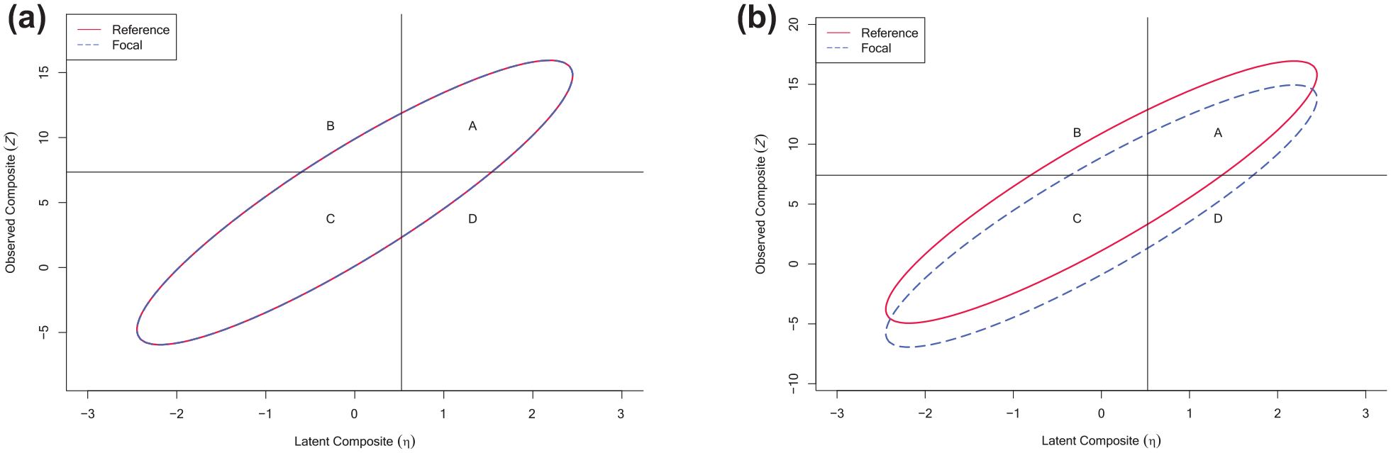
Distribution of Observed and Latent Scores by Group and Invariance Condition: (a) Strict Factorial Invariance and (b) Partial Factorial Invariance
The proportion of decisions in each category (i.e., TP, FP, TN, and FN) may then be used to compute summary classification accuracy indices 2 (CAI): proportion selected (PS), success ratio (SR), sensitivity (SE), and specificity (SP; Millsap & Kwok, 2004). Proportion selected,

refers to the ratio of individuals who screened positive over the number of individuals assessed. Success ratio,

(also termed positive predictive value or the precision of a test; Mohan et al., 2021) indicates the proportion of positive screens who are truly at risk of depression. Sensitivity,

is also known as true positive rate, hit rate, or recall (Mohan et al., 2021), and refers to the success of the test in capturing individuals who meet the criteria: out of all the individuals who should be identified as at risk, how many of them actually screened positive? Finally, specificity,

(selectivity or true negative rate), corresponds to the ability of the test in screening out the individuals who should have been excluded.
Under the simplifying assumption that individuals belong to one of two distinct populations (termed the focal and reference groups, where the reference group often corresponds to the majority group), the classification accuracy analysis framework entails the computation and comparison of CAI for the reference and focal groups under MI versus PMI to better understand the extent and practical impact of bias on test performance. If the negative impact of noninvariant items is deemed large enough by the test user, Millsap and Kwok (2004) suggest solutions such as removing noninvariant items or using a different test, and state that such decisions should be made with the usage of the test and the cost of each type of misclassification in mind. For instance, FPs and therefore SR and SP might be of greater concern if the test will be used to give access to limited and costly resources (Millsap & Kwok, 2004).
When MI holds and the latent distributions are equal, we expect equal TP, FP, FN, and TN proportions for the reference and focal groups. However, proportions may be drastically different across groups under PMI (see Figure 1). Furthermore, if the latent distributions are not equal across groups, it is not possible to compare the indices across groups even under MI. To address this concern, an additional set of indices termed “expected focal” (Efocal) can be computed as the proportions we would expect to observe for the focal group if its latent distribution matched that of the reference group. One index of note based on this idea is the AI ratio (Nye & Drasgow, 2011; Stark et al., 2004), which refers to the ratio of the expected proportion selected for the focal group and the observed proportion selected for the reference group. The AI ratio was developed to quantify the impact of differential item functioning on selection outcomes and can be computed within Millsap and Kwok’s (2004) original framework.
The main idea behind the AI ratio is that if the latent trait level is equal across groups, the proportions of individuals scoring above the threshold should be equal in each group, which allows us to attribute any differences between selection proportions to measurement bias. Conditioning on the latent trait level
The AI ratio is defined as

(Nye & Drasgow, 2011; Stark et al., 2004) which we express as

where PS r denotes PS for the reference group, and PS Ef denotes the expected PS for the focal group if both groups were matched to have the latent score distribution of the reference group. If SFI holds, the expected PS for the focal group will be equal to the PS for the reference group; hence, the AI ratio will equal 1. Deviations from 1 indicate the presence of measurement bias. A commonly used rule is the “four-fifths” rule, which suggests that the focal group has suffered AI if the AI ratio falls below 0.80 (Biddle, 2006; Nye & Drasgow, 2011). In an AI situation, the item with the removal of which brings the AI ratio the closest to 1 would be our candidate for deletion.
The Multidimensional Classification Accuracy Analysis Framework
Noting that selection and classification decisions are rarely based on psychological tests measuring a single, unidimensional latent construct, and that different weights may be assigned to different dimensions in practice, Lai and Zhang (2022) expanded the selection accuracy analysis framework (Millsap & Kwok, 2004) to work with tests aimed to measure multiple latent constructs with different weights. Assuming the multivariate normality of the latent factor scores and the unique factor variables, the observed composite scores Zg and the latent composite factor scores η g (where the latent composite is a weighted combination of the latent dimensions and g denotes group membership) were shown to follow a bivariate normal distribution (see Appendix A; Lai & Zhang, 2022). Furthermore, the marginal distribution of (Z, η) was demonstrated to be a finite mixture of bivariate normal distributions with mixing proportion π g , and the latent composite cut-off η c can be computed as the quantile in the mixture corresponding to PStotal (Lai & Zhang, 2022; Millsap & Kwok, 2004). The researcher may choose to pre-specify PStotal (e.g., to select the top X% of candidates) or specify a cut-off Zc (e.g., in a diagnostic screening setting), which will then be used to compute the proportion of individuals selected using the cut-off.
While this framework helps test users to link measurement noninvariance to the practical impact on classification, it does not provide clear methods for or guidance on how test accuracy and fairness may be improved, for example, by dropping biased items. Our goal is to remedy this gap by providing test users with item deletion indices that allow for the assessment of improvements (or decreases) in test accuracy and fairness when a biased item is dropped.
Methods: Item Deletion
The methods discussed here concern the case where a psychological test used for classification decisions contains measurement bias, and the researcher aims to investigate which of the test items, if any, may be deleted to reduce the negative impact of this bias on the performance and fairness of the scale. The deletion of an item may not be necessary or beneficial in some scenarios, and may in fact harm the validity and reliability of the test as will be discussed later. The methods outlined here are provided to facilitate researchers’ exploration of their data and to lead to more informed decisions about deleting or retaining an item.
The test instrument can consist of a single factor (e.g., depressive affect) or multiple factors (e.g., a scale of depression measuring different facets of depression such as positive affect, negative affect, and somatic symptoms). In this paper and in the accompanying unbiasr package, deletion is considered in a step-wise manner such that no more than one item is to be dropped at one time. Unless otherwise indicated by a subscript (e.g., SE sfi ), we assume that CAI is computed under PFI. The current method assumes that each item loads onto a single factor (i.e., no cross-loadings).
We can examine the impact of dropping an item on the difference in CAI from three distinct but complementary angles. The first approach entails an examination of an overall measure of classification accuracy, termed aggregate CAI (
We now introduce h and Δh, operations used to compute item deletion indices that quantify differences in CAI and
Operation: Cohen’s h (Cohen, 1988)
Cohen’s h (1988) is an effect size measure of the difference in two proportions or probabilities that was designed to account for the fact that probabilities can only range from 0 to 1, and uses the arcsine transformation so that the values better resemble an interval scale. Cohen’s h (1988) effect size of the difference between proportions p1 and p2 is defined as

Resulting h values can be interpreted as indicators of small, medium, or large differences between proportions using the conventionally used benchmarks of 0.2, 0.5, and 0.8 (Cohen, 1988). For example, if p1 = 0.65 and p2 = 0.50, we have h(0.65, 0.50) = 0.30, which corresponds to a small-medium effect size, and h(0.95, 0.80) = 0.48.
Operation: Delta h (Δh)
The change in the effect size h when a noninvariant item j is deleted is also of interest. Using * as a placeholder for the comparison h was computed for, the operation Δh is defined as

Delta h can be used to quantify the change in the difference between h values comparing CAI across groups or invariance conditions when the jth item is dropped. As an example, consider a scenario where we are interested in the change in the effect size h associated with the difference between SE
r
and the SE
Ef
computed when item 2 is deleted (

Second, h for the difference between
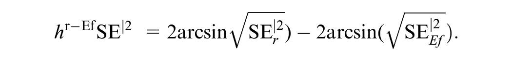
Finally, these values are compared using

Note that Delta h is only computed on h values, in contrast to Cohen’s h which can be computed for “raw” proportions. Having defined these two operations, we now describe the first three approaches to item deletion in more detail.
Approach 1: Examining Changes in Aggregate Classification Accuracy Indices (
)
We obtain aggregate classification accuracy indices as weighted averages across groups (see Appendix B for computation details) and
We suggest that the item j leads to the largest increase in
Approach 2: Examining the AI Ratio
We then compare the AI ratio computed using the full item set (AI) to the one computed using the item set excluding biased item j (AI|j). If the deletion of j does not lead to an AI|j closer to 1 than AI for any j, or leads to an AI ratio that is lower than the one computed using the full item set, all items should be retained as the deletion of items has no impact or leads to more AI. If, on the other hand, the deletion of item j brings the AI ratio closer to 1, the discrepancy between PS r and PS Ef has decreased, signaling an improvement. If in fact AI|j = 1, we can say that the difference between the groups in PS that is due to measurement bias is eliminated as the deletion of item j achieves a PS f that is equivalent to that of the PS r if these two groups were matched on their latent trait level. If there are multiple items the deletion of which leads to an improvement, the researcher is advised to consider the deletion of the item that brings the AI ratio the closest to 1. If multiple items lead to a similar improvement in the AI ratio if deleted, the researcher may continue their exploration of the other indices and make a judgment call as to which item, if any, should be deleted.
Approach 3: Examining Differences in CAI for Reference and Efocal Groups
Comparisons can then be made between the observed scores for the reference group (CAI
r
) and the scores we would expect to see for the focal group if the focal group followed the same distribution as the reference group (CAI
Ef
) by conditioning on the matched latent trait. Unlike the AI ratio, which focuses solely on PS, this approach allows the researcher to quantify discrepancies between SE
r
, SR
r
, and SP
r
, and SE
Ef
, SR
Ef
, and SP
Ef
, and to interpret any observed difference between
After computing Cohen’s h values for the difference between CAI
r
and CAI
Ef
for the full item set (hr-EfCAI) and an item set excluding biased item j (hh-Ef
The three approaches are intended to be examined in conjunction, and test users are advised to compare and contrast results from each approach before making a final decision about item deletion. If there is unanimity across the approaches supporting the deletion of an item (and assuming that its deletion does not have a major impact on the conceptual breadth of the test), the item may be dropped. If the three approaches agree, but the improvement as indicated by the indices is minimal, the test user may opt to retain the item in order to preserve the statistical properties and construct coverage of the scale. If there is disagreement between the approaches such that, for example, one approach indicates an improvement and one approach indicates a decrease in accuracy and fairness if an item is deleted, the user is advised to proceed with caution and examine raw classification accuracy indices. We suggest that items should be retained unless there is a clear indication that the deletion of an item would lead to a concrete improvement and would not harm accuracy and fairness.
Illustrative Example
We now illustrate the use and interpretation of the item-level deletion indices in a diagnostic application context using CFA estimates from a previous study investigating the MI of the CES-D (Radloff, 1977) across Chinese and Dutch elderly populations (Zhang et al., 2011). CES-D is made up of 20 items and four factors: positive affect (good, hopeful, happy, enjoyed), depressive affect (blues, depressed, failure, fearful, lonely, crying, sad), somatic complaints (bothered, appetite, mind, effort, sleep, talk, get going), and interpersonal problems (unfriendly, dislike). Participants are asked to rate each item on a scale of 0 to 3 based on how they felt in the past week. The maximum score is 60 on the full scale.
In their examination of data collected from 4,903 elderly adults from China and 1,903 elderly adults from the Netherlands, Zhang and colleagues (2011) found that configural and metric invariance held, and demonstrated partial scalar and partial strict invariance such that while the same construct was being measured across groups, there were differences in intercepts (failure, good) and uniqueness (depressed, fearful, and dislike). Depending on the size and direction of these differences, more individuals from the Chinese elderly (reference) group may be flagged for depression, resulting in a potential waste of valuable and limited resources. Likewise, fewer individuals from the Dutch elderly (focal) group who are truly at risk for depression may screen positive, which may mean that their treatment is delayed, or they lose access to resources or interventions. These observed differences may also be mistaken for true group-level differences, leading to spurious conclusions in theory building which may have unforeseeable downstream consequences. Taking informed steps to delete the item introducing the most bias to the scale may allow practitioners and researchers to mitigate unfair disadvantages caused by measurement bias.
We demonstrate the item deletion framework assuming that the CES-D scale is used as an initial screener for risk of depression, where selected individuals would be further assessed by a clinician who may leverage multiple additional information sources (e.g., a diagnostic interview) to determine whether the individual qualifies for some treatment or intervention program for depression. We use unstandardized factor loading, uniqueness, intercept, factor mean and factor standard deviation estimates from Zhang et al. (2011) and a latent factor variance-covariance matrix computed using factor correlation estimates from a previous study by Miller et al. (1997) as our input parameters. 4
We use a cut-off score of 16 on the full CES-D scale following the example of Radloff (1977) and hold the proportions selected using the full set of items constant in the item deletion scenarios considered. Note that researchers can instead choose to provide a new post-deletion cut-off to be used.
The mixing proportion π r is set to 4,903/(1,903 + 4,903) ≈ 0.72. As the depressive affect and somatic affect factors have seven items each, the lack of positive affect factor has four items, and the interpersonal problems factor has two items, this allocation of weights results in 35%, 35%, 20%, and 10% weighting for the aforementioned latent dimensions. All relevant parameter values, function calls, and outputs can be found in the code excerpts included in the Supplemental Material. 5
Item Deletion on the 20-Item, Four-Factor CES-D Scale
Under PFI, PS = 0.457 of the Chinese elderly group and PS = 0.144 of the Dutch elderly group scored above the cut-off score of Zc = 16, which corresponds to an aggregated
Items 4, 9, 10, 11, 15, and 20 (effort, depressed, failure, fearful, good, and dislike, respectively) were identified as biased by Zhang et al. (2011). Table 1 illustrates the
Aggregate Classification Accuracy Indices and h Values Computed for the 20-Item CES-D Scale.
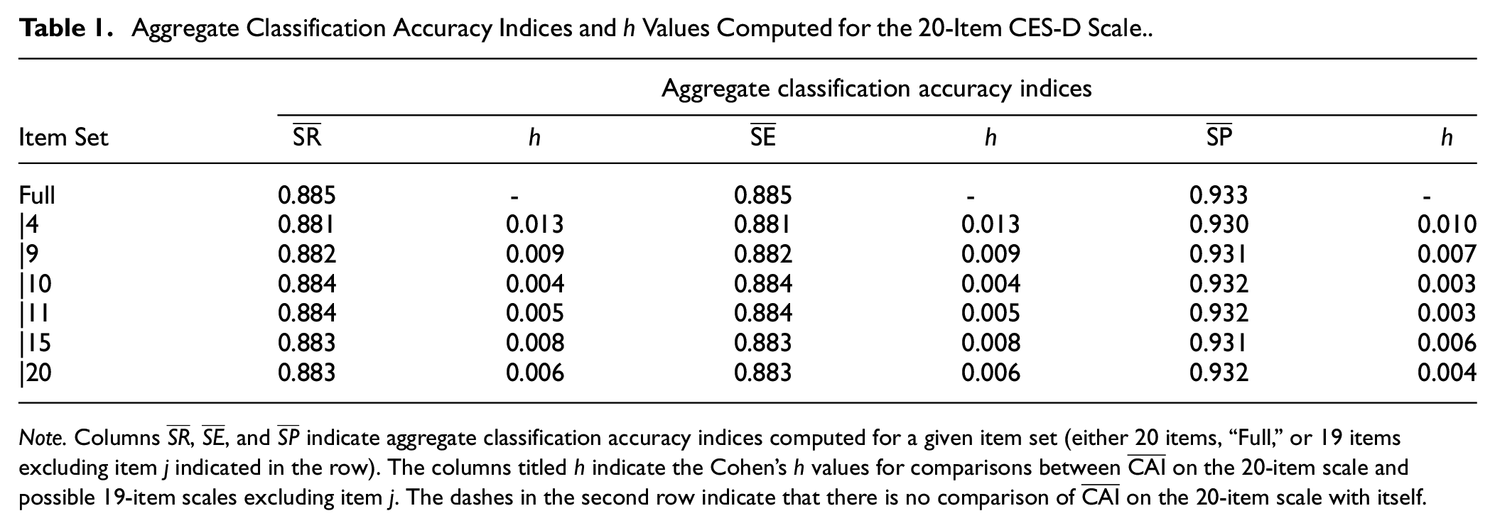
Note. Columns
Table 2 contains the item deletion indices quantifying the discrepancy between CAI r and CAI Ef . The AI ratio for the full scale is AI = 0.908, which is greater than the 80% threshold for adverse impact. The deletion of item 9 (depressed) or 11 (fearful) leads to AI ratios further away from the optimal ratio of 1, whereas deleting item 4 (effort) or 20 (dislike) leads to no change in the AI ratio. The greatest improvement in the AI ratio is observed for the removal of item 15 (good), followed by item 10 (failure) as the removal of either item brings the AI ratio closer to 1: AI|15 = 0.977 and AI|10 = 0.930. The rightmost three columns of Table 2 illustrate the effect size of the discrepancies between CAI r and CAI Ef attributable to measurement bias. hr-EfSR = −0.157 and hr-EfSP = −0.164 on the full CES-D scale suggests higher SR and SP values for the focal group (Dutch elderly) had the focal group been matched with the reference group (Chinese elderly) on the latent traits. Similarly, hr-EfSE = 0.141 suggests a lower SE for the expected focal group. Not only does the deletion of item 15 (good) attenuate the discrepancy between CAI r and CAI Ef , bringing the h values closer to 0 (h|15SR = −0.047, h|15SE = 0.026, h|15SP = −0.048), improvements caused by the deletion of this item also have the largest effect sizes out of all item deletion scenarios (Δh|15SR = 0.110, Δh|15SE = 0.116, Δh|15SP = 0.116).
Item Deletion Indices Comparing the Reference and the (Expected) Focal Groups on the 20-Item CES-D Scale.
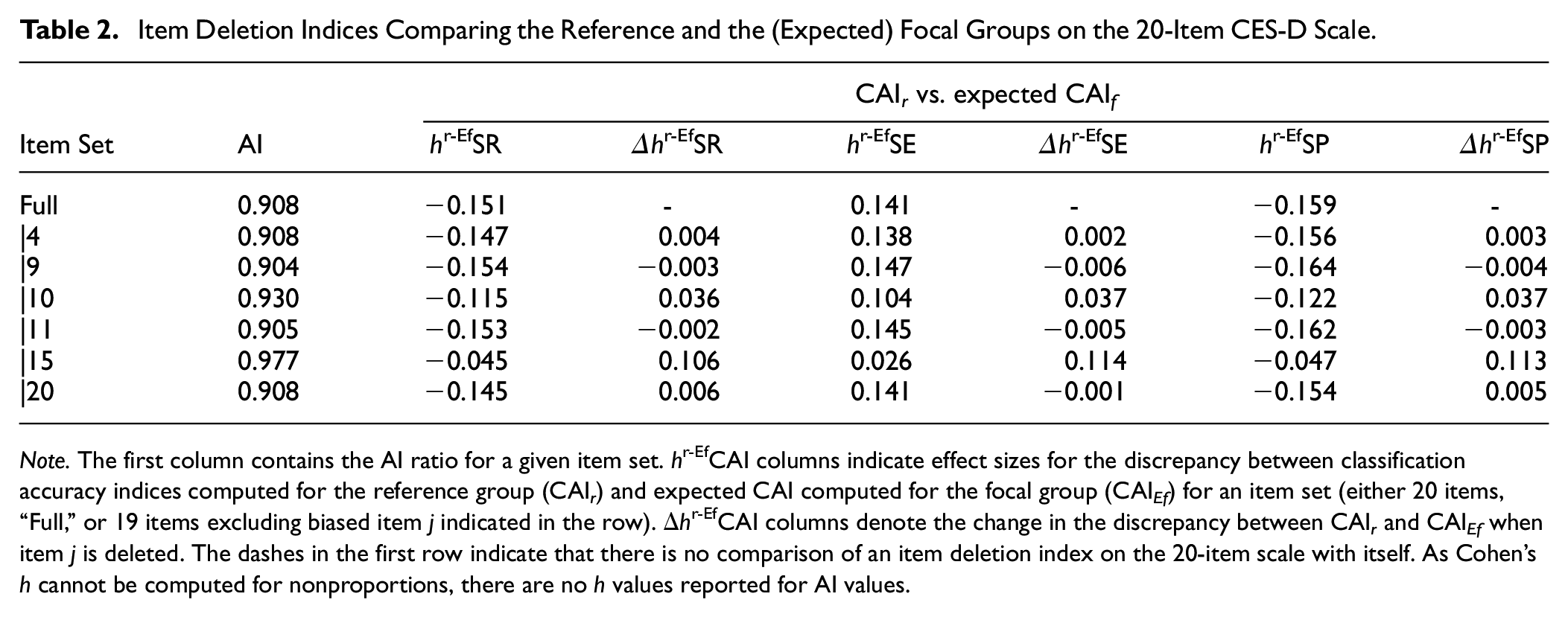
Note. The first column contains the AI ratio for a given item set. hr-EfCAI columns indicate effect sizes for the discrepancy between classification accuracy indices computed for the reference group (CAI r ) and expected CAI computed for the focal group (CAI Ef ) for an item set (either 20 items, “Full,” or 19 items excluding biased item j indicated in the row). Δhr-EfCAI columns denote the change in the discrepancy between CAI r and CAI Ef when item j is deleted. The dashes in the first row indicate that there is no comparison of an item deletion index on the 20-item scale with itself. As Cohen’s h cannot be computed for nonproportions, there are no h values reported for AI values.
In light of these findings, and barring any domain-specific reasons to retain this item, we can conclude that deleting item 15 would help mitigate the impact of measurement bias on classification accuracy and fairness, and render the diagnostic accuracy of the CES-D for the Chinese and Dutch elderly groups more comparable (see the Supplemental Material for an illustration of the distributions of latent and observed scores for depression for the Dutch and Chinese elderly groups before and after the deletion of item 15).
We would like to emphasize that the suggestion to delete item 15 (good) only applies to the findings discussed here by Zhang et al. (2011) regarding the comparison between Chinese and Dutch elderly individuals, and does not necessarily generalize to item or test performance in other contexts. For instance, if a clinician is adapting the Chinese version of the CES-D to screen depression risk for their clients, we would recommend repeating the analyses here with their data and carefully examining the performance of all items including item 15 before proceeding with any deletion.
Four-Factor CES-D Scale After Deleting Item 15
Continuing with the diagnostic example, we perform item deletion on the remaining 19 items of the CES-D to see whether the deletion of a second item may further reduce the impact of measurement bias. The cut-off score is recomputed as Zc = 16/60 × (60−3) = 15.2 to account for the deleted item. Results are illustrated in Tables 3 and 4.
Aggregate Classification Accuracy Indices Computed for the 19-Item CES-D Scale.
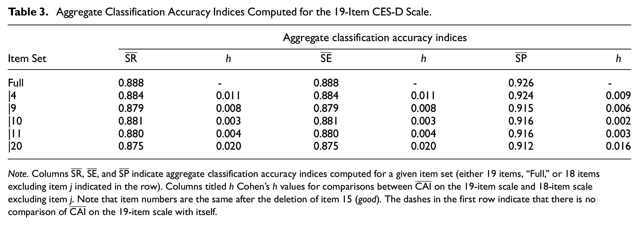
Note. Columns
Item Deletion Indices Comparing the Reference and the (Expected) Focal Groups on the 19-Item CES-D Scale.
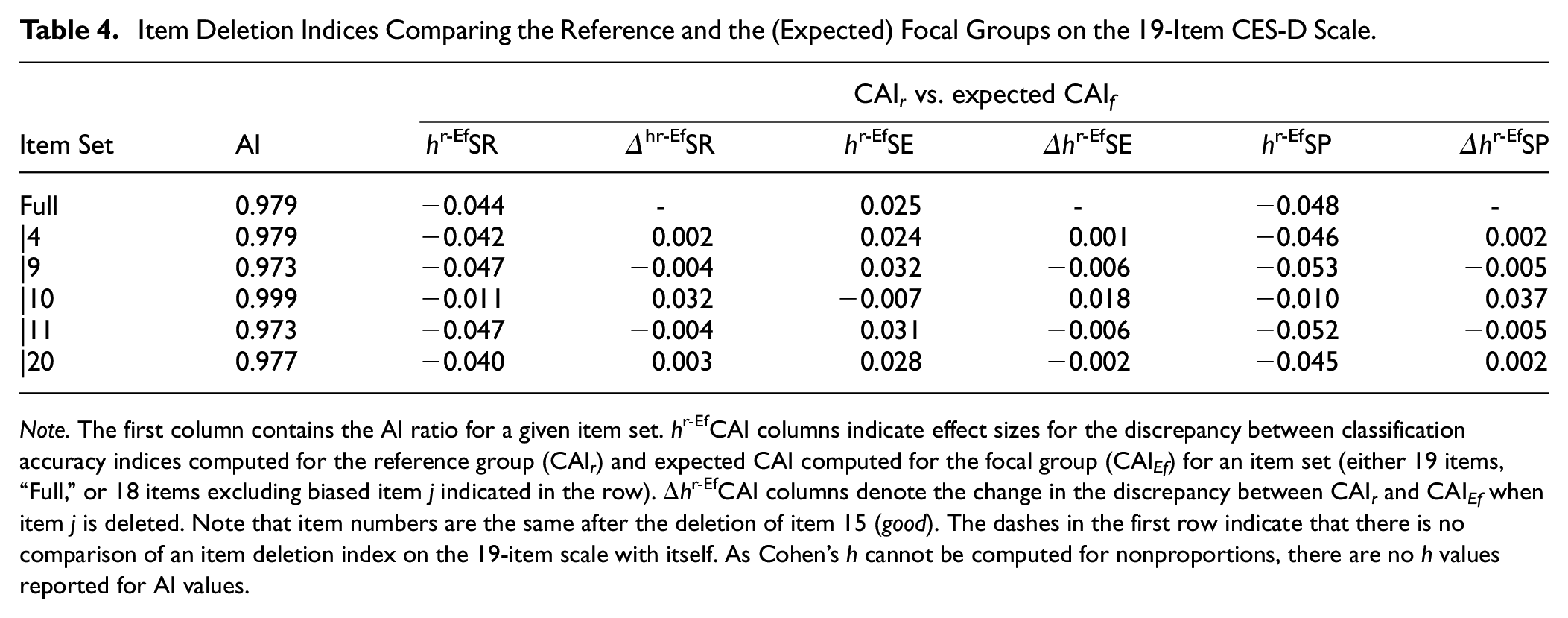
Note. The first column contains the AI ratio for a given item set. hr-EfCAI columns indicate effect sizes for the discrepancy between classification accuracy indices computed for the reference group (CAI r ) and expected CAI computed for the focal group (CAI Ef ) for an item set (either 19 items, “Full,” or 18 items excluding biased item j indicated in the row). Δhr-EfCAI columns denote the change in the discrepancy between CAI r and CAI Ef when item j is deleted. Note that item numbers are the same after the deletion of item 15 (good). The dashes in the first row indicate that there is no comparison of an item deletion index on the 19-item scale with itself. As Cohen’s h cannot be computed for nonproportions, there are no h values reported for AI values.
In Table 3, we see that the deletion of any of the remaining biased items (4, 9, 10, 11, 20, or effort, depressed, failure, fearful, dislike) leads to decreases from
In the first column of Table 4, only item 10 (failure) leads to an AI ratio that is closer to 1 if deleted, with AI|10 = 0.999 from AI = 0.979. 6 In the next three columns of Table 4, we see that deleting item 10 may also slightly reduce the discrepancy between CAI r and CAI Ef , with hr-EfSR|10 = −0.011, hr-Ef SE|10 = −0.007, and hr-EfSP|10 = −0.011. The effect sizes of these changes in a discrepancy between CAI r and CAI Ef are Δh|10SR = 0.032, Δh|10 SE = 0.017, and Δh|10SP = 0.036. The deletion of any other item either leads to an insubstantial improvement or exacerbates the discrepancy between CAI r and expected CAI f , increasing bias.
While these results show that item 10 introduces the most bias after item 15, the potential improvement achieved from dropping this item is not as clear-cut as that from the deletion of item 15. Given the ambiguity of these results and the lower magnitude of the improvements in AI and hr-EfCAI compared to when item 15 was the candidate for deletion, we would recommend retaining item 10 and proceeding with the 19-item CES-D scale unless further, theory-based justification supporting the deletion of item 10 is established. It may be worthwhile examining the raw classification accuracy indices as, depending on the application context, whether an increase in SR is caused by a decrease in FP or an increase in TP may give additional insight into the best course of action if the scale will be used for allocating limited resources such as access to a treatment program. We believe that the methods and guidelines outlined here equip test users to make more informed decisions about whether improvements in AI and hr-Ef CAI are large enough to warrant item deletion.
Implementation Using R Package unbiasr
The R package unbiasr implements the item deletion methods proposed in this paper. The main function in unbiasr is PartInv(), which allows users to evaluate the practical impact of classification accuracy across groups and requires only the CFA parameter estimates as input. item_deletion_h() computes effect size indices quantifying the impact of deleting biased item(s) on classification accuracy indices. unbiasr incorporates the R scripts from Lai et al. (2017) and Lai and Zhang (2022).
First, CAI is computed under SFI and PFI for the full set of items using the user-specified item weights. Then, summary statistics are computed for the item set excluding item j using an adjusted item weight vector where an item weight of zero is assigned to the jth item. In the calculation of the new item weights, the weight that had been allocated to the jth item is redistributed across the remaining test items proportionally to the current weights of these items. If the test is multidimensional, the weighting is redistributed only across the items that belong to the same subscale as item j. Once relevant delete-one classification accuracy indices are computed for the reference, focal, and expected focal groups under SFI and PFI, operations h and Delta h are used to compute the deletion indices (
Depending on the purpose and application context of the test, users may indicate a cut-off score (Zc; e.g., to identify patients scoring above a clinically meaningful cut-off for treatment referral), or input a proportion for selection (propsel; e.g., to hire the candidates scoring in the top 10% of the applicant pool). If the user specifies a cut-off Zc as well as a delete-one cut-off score adjusting for the decrease in the maximum total score when an item is dropped from the scale, the second cut-off score is used as the new Zc in item deletion scenarios. If the user specifies a proportion for selection, this value is held constant in item deletion scenarios. If a delete-one cut-off score is not provided by the user, the PS sfi and PS pfi using Zc on the full item set are held constant in the computations of CAI in item deletion scenarios. For example, if Zc = 16 on the full scale corresponds to PS sfi = 0.30 and PS pfi = 0.28, summary statistics will be computed with propsel = 0.30 and propsel = 0.28 so that the highest scoring 30% and 28% of individuals in each item deletion scenario will be selected under strict and partial invariance conditions, respectively.
Discussion
Psychological tests provide decision-making bodies and scientists alike with a relatively time-efficient and objective tool for the assessment and comparison of individuals’ relative standings on constructs of interest and are used in a range of applications from theory construction and advancement to decision-making. As such tests are commonly used in high-stakes contexts and may have wide-reaching consequences beyond the immediate application of the test, it is critical that test scores are valid and free of bias. A notion inextricably linked to validity and bias is MI, which holds when a test measures the same construct in the same way across grouping variables that are irrelevant to the construct under study (e.g., race). The current framework provides decision-makers with tools and guidelines to better navigate the seldom-discussed next steps following the discovery of noninvariant items.
We have fully automated the three complementary approaches to item deletion outlined in this paper, and the functions for the computation of item deletion indices are available in our open-source R package unbiasr. The outlined methods expedite and give structure to the otherwise laborious and error-prone process of determining the best course of action to handle item bias by converting differences in classification accuracy indices to comparable and easily interpretable units. As such, test users can make more informed decisions about item deletion (or retention) more efficiently, prevent the misallocation of limited resources, expedite the time it takes for patients to receive the care they need, and reduce the influence of construct-irrelevant factors on classification decisions, promoting fairness. We hope that the detailed examination and discussion of the item deletion indices in the illustrative example helps elucidate the process of determining whether a biased item can, or should, be deleted to improve accuracy and fairness in classification decisions.
There are a number of limitations to the current work. First, the methods outlined here concern binary classification decisions, such as selection versus rejection or diagnosis versus no diagnosis. Future work is planned to extend to classification into multiple categories (e.g., classification of an individual’s depression level into severity categories; class placement of students based on levels of language proficiency). Second, we only considered noninvariance across two groups, whereas many demographic characteristics have multiple subgroups (e.g., ethnicity, race, SES). We hope to extend the framework to the classification of individuals across multiple groups. Third, we assumed that the test items were measured on an interval scale. We have proposed and illustrated the current framework in the context of interval level data, 7 but we plan to extend the framework to ordered categorical data in future research. Moreover, the current methods do not quantify the uncertainty around the estimates. Additional tasks for our package therefore include extending the current methods to performing item deletion for multiple groups as well as for when test items may be measured on a binary or ordinal scale, and computing uncertainty estimates (e.g., Bayesian credible intervals).
Any item deletion decision should be made with the context and application of the test in mind (Millsap & Kwok, 2004), as one potential consequence of deleting items is reduced construct coverage (Kruyen et al., 2013). While the deletion of an item may lead to better classification accuracy and increased fairness, the item may nevertheless be important to retain, particularly in application contexts where inference and interpretability take precedence over prediction. It may be more important in a research context to get a holistic picture that taps into all facets of the construct for theory-building purposes as opposed to in more applied contexts where the goal is to make a decision. 8 For example, imagine the item loss of interest and pleasure, which measures an aspect of depression that is integral to the construct definition of depression, is found noninvariant across groups and that the deletion of this item leads to better classification accuracy and higher fairness. If the goal is to determine the individuals who qualify for a treatment program, the improvement in performance and fairness in outcomes may justify the deletion of the item as the predictive validity of the scale as a diagnostic tool may be of greater interest. However, if the scores on the depression scale are, for example, used to gain a better understanding of the manifestation of the symptoms of depression in different cultural contexts, we recommend consulting existing literature as well as domain experts to clarify the potential reductions in construct coverage. It may also be worthwhile to explore alternative approaches, such as going back to the drawing table and piloting modified versions of the noninvariant item with samples from the different groups to rebuild the scale with an unbiased replacement item, assuming that resource and time constraints allow for such a detour.
Furthermore, test users should exercise great caution while considering deleting multiple items at a time from a scale, and note the close relationship between the test length and its internal reliability (Brown, 1910; Kruyen et al., 2012; Spearman, 1910). We stress that the shorter the test, the riskier it may be to drop items.
The item deletion indices, methods, and guidelines introduced here function as exploratory tools to scrutinize the “what-if” scenarios concerning biased items. It is ultimately up to the decision-maker to judge whether the magnitude of an improvement is large enough to warrant deletion and determine whether one or more items, if any, can (and should) be deleted in a given application context.
Supplemental Material
sj-docx-1-asm-10.1177_10731911241298081 – Supplemental material for Exploring the Impact of Deleting (or Retaining) a Biased Item: A Procedure Based on Classification Accuracy
Supplemental material, sj-docx-1-asm-10.1177_10731911241298081 for Exploring the Impact of Deleting (or Retaining) a Biased Item: A Procedure Based on Classification Accuracy by Meltem Ozcan and Mark H. C. Lai in Assessment
Footnotes
Appendix A
Appendix B
Declaration of Conflicting Interests
The author(s) declared no potential conflicts of interest with respect to the research, authorship, and/or publication of this article.
Funding
The author(s) disclosed receipt of the following financial support for the research, authorship, and/or publication of this article: This work was sponsored by the U.S. Army Research Institute for the Behavioral and Social Sciences (ARI) and was accomplished under Grant #W911NF-20-1-0282. The views, opinions, and/or findings contained in this paper are those of the authors and shall not be construed as an official Department of the Army position, policy, or decision, unless so designated by other documents.
Supplemental Material
Supplemental material for this article is available online.
Notes
References
Supplementary Material
Please find the following supplemental material available below.
For Open Access articles published under a Creative Commons License, all supplemental material carries the same license as the article it is associated with.
For non-Open Access articles published, all supplemental material carries a non-exclusive license, and permission requests for re-use of supplemental material or any part of supplemental material shall be sent directly to the copyright owner as specified in the copyright notice associated with the article.