Spurious Reliability Increase?: The Number of Response Options in the Likert-Type Scale Influences Only Internal Consistency,Not Criterion Validity

Abstract

The existing research on the number of options in the Likert-type response format has focused primarily on reliability and descriptive statistics, often overlooking validity or examining it with limitations. This study addressed this gap through a within-subject experiment (N = 846, 69% women), manipulating response options (two, six, and 10) in two Likert-type scales: the Height Inventory and the autonomy subscale of the Basic Needs Satisfaction in General Scale. Two-point variants significantly differed in means and reliability compared to six- and 10-point versions. While the magnitudes of differences were small in Height Inventory, it did not follow for the autonomy subscale. On the other hand, validity (criterion, measurement model, and trait criterion validity) remained unaffected. Thus, the increased reliability may be spurious, stemming from systematic but construct-irrelevant variance related to response format (i.e., method variance). These findings suggest that response formats with fewer options can be viable, particularly in scales with more items. Future research should explore differences in cognitive processes across response formats.

Keywords

Likert-type scale measurement invariance criterion validity reliability number of response options measurement model

Introduction

Does the number of response options on the Likert-type scale matter? Although the original scale assessing attitudes was initially developed with five response categories (Likert, 1932), researchers have used a varied number of response options (note that in this paper, the terms response categories/options/points are used interchangeably). Researchers have extensively examined the influence of the number of response categories on the psychometric properties of questionnaires; thus, it might seem there is nothing new that we could learn on this topic. However, most of the research has focused on testing differences in means and internal consistency at the expense of what the issue of response format is really about – validity. To address this gap, we proposed an innovative within-subject methodological approach to differentiate various sources of response variance. Our approach’s main advantage was that it used an objective attribute, specifically, human height, the value of which is known with high precision and which has proven helpful in similar research (Borsboom et al., 2002; Kam et al., 2021).

Internal Consistency: Cronbach’s Alpha Stealing the Show

An increase in systematic variance (i.e., the variance associated with a true score, $σ_{τ}^{2}$ ) or a decrease in random error variance ( $σ_{e}^{2})$ increases reliability ( $ρ_{x x'}$ ), as expressed by the following well-known formula:

ρ_{x x'} = \frac{σ_{τ}^{2}}{σ_{τ}^{2} + σ_{e}^{2}} = 1 - \frac{σ_{e}^{2}}{σ_{x}^{2}}

(1)

Intuitively, providing more response options should lead to more nuanced replies and more information, thus increasing systematic variance in responses. Therefore, reliability should grow with a greater number of response options in the Likert-type response format, as demonstrated in several simulation studies (Bandalos & Enders, 1996; Lee & Paek, 2014; Lozano et al., 2008). Empirically, reliability (especially internal consistency) has been the most studied aspect when comparing Likert scales with different number of response options. The knowledge in this area is relatively robust, as studies have consistently reported a similar pattern, reporting that Cronbach’s alpha increases with the inclusion of up to five or six response options (Hilbert et al., 2015; Muñiz et al., 2005; Simms et al., 2019; Weng, 2004) and then levels off (Muñiz et al., 2005; Simms et al., 2019) or even declines (Bendig, 1953; Chang, 1994; Preston & Colman, 2000). Moreover, an odd number of response options seems to perform below the expected trend, while an even number of options performs better (Nadler et al., 2015).

Some studies have not found any increase with the addition of up to five or six points or even any relationship between the number of options and reliability (Bendig, 1953; Jacoby & Matell, 1971; Leung, 2011; Preston & Colman, 2000; Xu & Leung, 2018). Some of these contradicting results can be explained by suboptimal design (Bendig, 1953), small sample sizes (Bendig, 1953; Leung, 2011) or expected small effect sizes (and thus low power) when comparing only four response options with the 5, 6, or 11 (Leung, 2011).

Generally, two-point scales have lower internal consistency than variants with more points (Hilbert et al., 2015; Simms et al., 2019), which is evident given the limited variance of shorter response formats. On the other hand, when relaxing the tau-equivalency of Cronbach’s alpha using less biased McDonald’s omega (see Sijtsma, 2009; Sijtsma & Pfadt, 2021a, 2021b, for a detailed discussion), the differences in reliability between two-point and five-point scales disappear (Hilbert et al., 2015).

Validity: Entering the Scene

Although reliability is an important aspect to consider in questionnaire development, we argue that the issue of response format is primarily an issue of validity. Previous research has touched on the problem, although it has focused mainly on correlations with distantly related criteria, such as school attendance (e.g., Hilbert et al., 2015) or other psychological constructs measured with limited validity and reliability. The results seem reassuring, as they suggest no significant differences in convergent (Cox et al., 2012; Preston & Colman, 2000), predictive and concurrent (Jacoby & Matell, 1971; Jones & Loe, 2013; Leung, 2011), or criterion validity (Chang, 1994; Hilbert et al., 2015).

However, choosing a good criterion in research on validity is more challenging than meets the eye. What should such a criterion fulfil? First, the systematic but construct-irrelevant variances (of the scale and the criterion) must be independent. Consider the following common example where researchers manipulate the number of response categories within one scale and examine changes in correlation between the sum scores from these variants and a sum score from a different Likert-type scale (i.e., a criterion). If the precision of measurement increases with the number of response categories, so should the criterion validity (i.e., correlation with the criterion). However, when using another Likert-type scale as a criterion, we cannot differentiate whether the increase is due to more precise measurement or an increase in the systematic but construct-irrelevant variance of the response format. For example, Weijters et al. (2010) found out that the number of response options influences the response style in participants, which can be the source of such construct-irrelevant variance shared across items. In other words, the two self-reports using the same response format might share the same systematic method variance that causes the increase in reliability in the first place. Second, the criterion also has to correlate strongly with observed scores, which would increase statistical power to detect any differences. One solution to both problems is having the objective criterion representing the measured attribute with almost perfect reliability (together ensuring strong correlation) and no shared method variance related to the response format. We elaborate on this idea below.

From the previous paragraph, it is evident that in establishing criterion validity, we need to account for all the factors that contribute to the correlation between measure and criterion. This is possible by explicitly working with the measurement model (of the measure, criterion, or both). Unfortunately, the existing research has scarcely addressed differences in the measurement model across the Likert-type response formats. To our knowledge, only Xu and Leung (2018) tackled differences in measurement models across response formats with varying numbers of response points, stating scalar invariance. Although their study provided important insights, they collected data at a single time and treated discrete ordinal Likert-type items as continuous in their CFA models, which are limitations we wanted to overcome.

This Study

In the previous chapter, we raised concerns about the quality of criteria used in past research examining differences in validity across Likert-type scales with varying numbers of response options. We argued that the Likert-type scale and criterion should share a minimal amount of method variance, the criterion should be sufficiently reliable, and the relationship between the measured attribute and criterion should be meaningful. Ideally, the criterion should serve as an objective representation of the measured attribute. However, such criteria are rarely available for psychological constructs or attributes.

To address this issue, we proposed using human height as the primary attribute and self-perceived height as its psychological proxy for studying differences across Likert-type scale formats. An inventory of self-perceived height offers several advantages in this context. First, for adults, height is relatively stable over time, ensuring that its level does not fluctuate. This stability allows for a longitudinal experimental design, providing sufficient certainty that differences in responses are mainly due to experimental manipulation (i.e., the number of response points) or random error. Second, an objective and highly reliable criterion, actual height, facilitates a meaningful evaluation of criterion validity. Third, the criterion is free from construct-irrelevant variance, such as method variance, related to Likert-type scale and response styles, ensuring that the validity of the results remains unthreatened in this aspect.

This study compared Likert-type scales with two, six, and 10 response options in terms of mean levels, internal consistency, and criterion validity. These metrics represent differences in central tendency, systematic variance in sum scores, and the relationship between observed scores and the criterion, respectively. Furthermore, we examined trait criterion validity using structural equation modelling to determine how the latent trait itself relates to the criterion when measurement error is controlled.

To ensure equivalence across the different scale formats, we assessed measurement invariance. This step was essential to verify that increasing the number of response options did not alter the latent structure of the construct – a necessary prerequisite for any subsequent psychometric comparisons or to gain deeper insight about how the number of response options influences the underlying measurement model.

Part of these findings (descriptive statistics, reliability, and measurement invariance) was further replicated using a traditional psychological construct: the need for autonomy. For this construct, criterion-related analyses were omitted due to the absence of a comparable objective criterion.

Based on the existing evidence, we assumed that the internal consistency of the two-point Likert-type scale would be lower compared to the six and 10 options, with no differences between the latter two. On the other hand, based on our argumentation above, we did not assume any differences in criterion validity or measurement model, assuming that the increase in reliability from two to six points and then levelling off is caused primarily by systematic construct-irrelevant variance.

Methods

Sample

The minimal sample size was determined to be 500 respondents, based on recommendations for using robust mean and variance adjusted weighted least squares (WLSMV) estimator on the scale with 10 response categories (Li, 2016). Furthermore, we expected approximately 30% dropout, hence aiming at approximately 750 respondents enrolling in the first wave. Initially, 876 participants were enrolled in the research in the first of three waves; 30 participants younger than 18 years of age were excluded since the research targeted only the adult population. Furthermore, some questionnaire responses were excluded due to unrealistic response times (less than 2 s spent responding to an item), too consistent response patterns (no variance within a questionnaire, except for two-point variants), the time between measurements exceeding 2 weeks, and more than half of the data missing.

The final sample comprised 846 Czech-speaking participants (69% women, n = 585) with an average age of 23.80 years (SD = 6.56; Md = 22, ranging from 18 to 63). Regarding the highest level of education attained, 6% (n = 50) of participants completed primary school, 68.5% (n = 580) completed high school, and 25.5% (n = 216) held a bachelor’s degree or higher. At the start of data collection, most respondents were students (76%, n = 651). In addition, 36% (n = 300) were employed, five were retired, and 13 were on maternity or paternity leave. Note that these categories are not mutually exclusive and may overlap.

The sample was recruited using unpaid social media posts within several Facebook groups, focusing mainly on university students with different backgrounds (social sciences, STEM), or interest groups (education, volunteering, marketing, psychology). Potential participants were informed about the study aims and procedure, and possibility of earning a small profit. After the last data collection, we randomly selected one participant who completed all three waves and rewarded them with 1,000 CZK (about 50 USD).

Materials

Height Inventory

Height Inventory (HI; Rečka, 2018) is a self-reported measurement tool for self-perceived height that has a solid theoretical justification (see Introduction) and an excellent criterion validity with respondents’ actual height (r > .87). Although using HI could appear impractical, its close relationship and comparability with an external criterion provide significant utility. The almost perfect reliability of the tool’s criterion (i.e., actual height or self-reported height), combined with high correlation to inventory sum scores, makes it a good methodological tool for assessing the magnitude of various effects that influence measurement, as it provides higher power to detect potential differences in conditions (see Introduction). Indeed, Kam et al. (2021) used a similar approach to study reversed items, whereas Borsboom et al. (2002) used their height questionnaire to demonstrate various kinds of DIF.

So far, the tool has been adapted only to the Czech environment. However, the official English translation of the full questionnaire alongside the Czech data is included in the R package ShinyItemAnalysis in the HeightInventory object (Martinková & Drabinová, 2019). The questionnaire contains several statements about everyday situations in which height is relevant. The items are formulated in such a way that they follow the structure and content of a traditional psychological questionnaire. For example, items ask about the observable consequences of the attribute in the world (“I am used to hearing comments about how tall I am” or “I have enough room for my legs when traveling by bus”), person’s self-evaluation related to the attribute (“I have an appropriate height for playing basketball or volleyball”), or person’s behaviour that is assumed to be directly related to the measured attribute (“I must often be careful to avoid bumping my head against a doorjamb or a low ceiling”). These types of items are not anomalies in psychological research.

The original questionnaire consisted of 26 items; however, we shortened the questionnaire for our purposes. Thus, we re-analysed Rečka’s (2018) original data using item analysis and unidimensional confirmatory factor analysis. The resulting scale contained 11 items and showed satisfactory psychometric properties. For the final set of items, see Online Supplement 1.

Autonomy Subscale of the Basic Needs Satisfaction in General Scale

Basic Needs Satisfaction in General Scale (BNSG-S, Gagné, 2003) is a self-report measure based on the Self-Determination Theory (SDT; Ryan & Deci, 2000). SDT assumes three basic needs: autonomy, competence, and relatedness. BNSG-S is a multidimensional measurement tool containing 21 items divided into three subscales assessing three basic needs. In the STD context, the need for autonomy resembles the subjective feeling of ownership of one’s actions and decisions (Deci & Ryan, 1985; Ryan & Deci, 2000). The autonomy subscale (AS) used in this study consists of seven items (see Online Supplement 1), three of which are worded negatively. Although the subscale is considered unidimensional for the target population (Ježek et al., 2016), some other studies have suggested reverse items might share some otherwise unexplained variance (Johnston & Finney, 2010).

Procedure

We employed a within-subject experimental design with measurements at three different time points (i.e., measurement occasions). Participants were randomly assigned to one of three experimental conditions where the number of points in the Likert-type response format was manipulated. Specifically, on one measurement occasion, a participant was presented with either two-, six-, or 10-point variants of HI and AS. The remaining experimental conditions were administered 1 week apart in the following order: six-point scales followed the two-point ones, the 10-point scale followed the six-point one, and the two-point scale followed the 10-point scale. Participants were also asked about their real height (used as a criterion for HI) on the first and last measurement occasion.

Regarding the response formats, the odd/even number of points was held constant to avoid effects related to including the middle point (Nadler et al., 2015). The inclusion of the middle point would require more measurement sessions to control its effect on psychometric properties, which could overload participants. The two-point response format was chosen as a baseline measurement, as the effect of a cognitive load, some response styles, or other biases should be minimal. The six-point scale was selected as a breakpoint because reliability should increase to six points and then level off (Simms et al., 2019). We added verbal anchors to all points, as an invariance study with only endpoint anchors has already been conducted (Xu & Leung, 2018). See Online Supplement, Table S1, for details on wording. The use of data in the current research project has been approved by the Research Ethics Committee of Masaryk University (EKV-2022-027).

Data Processing and Diagnostics

The participants in each experimental condition were comparable across measurement occasions, χ²(4) = 1.24, p = .872. Moreover, the men-women ratio, χ²(2) = .10, p = .953, and education, χ²(6) = 1.25, p = .975, remained the same across measurements. Regarding dropout, 64 % of the participants (n = 537) completed the second, and 59 % (n = 492) finished the third measurement wave. After removing cases where the interval between measurement occasions exceeded 14 days, the average period between measurement occasions was 8 days (M = 7.97, SD = 1.60 between T1 and T2; M = 7.69, SD = 1.11 between T2 and T3).

Data Analysis

For the HI, we conducted analyses separately for men and women due to the non-invariance of measurement (Rečka, 2018). The AS analyses were run for both genders together using R programming language (R Core Team, 2021), version 4.1.2, and following packages: psych (Revelle, 2024), MBESS (Kelley, 2007), lme4 (Bates et al., 2015), sjstats (Lüdecke, 2018), car (Fox & Weisberg, 2019), effsize (Torchiano, 2020), lavaan (Rosseel, 2012), semTools (Jorgensen et al., 2022), and ggplot2 (Wickham, 2016).

Differences in Descriptive Statistics

To compare differences in total score means and variances between each experimental condition, we transformed the data into a long format (each row represented a unique participant’s total score in a single experimental condition). We predicted total scores (converted to a 0–1 range) using the linear mixed model specification, where the experimental condition was a dummy variable (fixed effect, the six-point scale was used as a baseline) and participant ID as a random effect (intercept-only). Subsequently, we compared residual variance across experimental conditions using Levene’s test.

Differences in Reliability

We estimated the unidimensional ordinal confirmatory factor analysis (CFA) model using an adjusted weighted least squares (WLSMV) estimator in the laavan package (Rosseel, 2012). Subsequently, we computed McDonald’s omega coefficients for each variant utilising the semTools package (Jorgensen et al., 2022), applying Green and Yang’s (2009) correction, and subsequently, determined the differences between the coefficients. We bootstrapped this procedure on 1,000 samples to obtain standard errors and 95% confidence intervals and to compare estimates using z-tests.

Differences in Criterion Validity

The criterion validity of the observed scores across conditions was evaluated using multigroup (men and women separately) path analysis performed in a lavaan package. The total scores from the four HI experimental conditions were regressed on the external criterion (self-reported height in centimetres). We standardised all variables to avoid problems with different metrics and used robust maximum likelihood (MLR) as an estimator. The model that included all responses was analysed using full information maximum likelihood (FIML). We freely estimated covariances between residuals since the scores shared some variance due to the longitudinal design. Stepwise, we constrained the regression coefficients, residuals, and covariances to be equal across experimental conditions. The models were hierarchically compared using Satorra and Bentler’s (2001) method.

Differences in Measurement Model and Item Parameters

Next, we assessed the differences in the measurement model. Due to the small number of men in the sample, the analyses for HI were limited to women, while AS analyses were conducted on the entire sample.

Items loaded on factors based on the experimental condition (e.g., item 1 with two options loaded on factor for that condition). The residuals for items with the same wording but different response formats were also allowed to covary. Invariant models were identified following Wu and Estabrook’s (2016) suggestions, using the first item as a reference indicator instead of standardising latent variables. Due to varying response options across conditions, we deviated slightly from the standard model definition (see Online Supplement, Table S2). We used ordinal factor analysis estimated in the lavaan package with robust mean and variance adjusted weighted least squares (WLSMV) estimator and theta parameterisation. The missing data were handled with pairwise deletion.

We proceeded in three stages. First, we focused on the measurement model. After fitting the configural model, we gradually constrained item loadings to be the same across formats, corresponding thresholds, intercepts, and residual variances. Second, we fixed population parameters by setting latent means to zero and variances to 1 in all the conditions and eventually fixed latent covariances to 1 for a unidimensional model. Finally, we also constrained item residual covariances across formats. We compared all the nested models using Satorra and Bentler’s (2001) method, considering the change in approximate fit indices using the standard rules of thumb (Chen, 2007; Cheung & Rensvold, 2002; Putnick & Bornstein, 2016; Sass et al., 2014): ΔTLI, ΔRMSEA, and ΔSRMR smaller than approximately .015 in the undesirable direction still suggested non-invariant models.

Differences in Trait Criterion Validity

Finally, the structural model was specified by adding the actual height to the final invariant unidimensional model. Each factor was regressed on a centred height in metres as an external criterion, and the latent regression parameters and latent residual variances were constrained to the same values across the conditions. While not changing the measurement model, we started by releasing the parameters. First, we released covariances of latent variables, assuming that the model is not unidimensional. Subsequently, we released latent residual variances in all conditions, followed by the latent regression parameters. See Online Supplement, Table S3, for more details.

Transparency and Openness

We report how we determined our sample size, all data exclusions, all manipulations, and all measures in the study. The original dataset included participant self-esteem measurements that are not reported here. The raw anonymised data, analytic code, and the online supplement are available in the Open Science Framework and can be accessed at https://doi.org/10.17605/OSF.IO/X9UG7. This study’s design and its analysis were not preregistered.

Results

Mean Differences

Respondents reported their true height consistently across the measurement occasion (r_{T1, T3} = .997). The descriptive statistics for each questionnaire and its variants are in Table 1. As expected, the normalised HI total score means differed significantly for two- and six-point variants. The effect sizes were relatively small (for women, b = −.02, β = −.04, p <.001; for men, b = .02, β = .04, p = .019), suggesting a slight central tendency for the longer format. The six- and 10-point scales did not differ in normalised total scores (for women, b = −.001, β = −.001, p = .956; for men, b = .004, β = .009, p = .568). Variances were significantly different across all three conditions (Levene’s tests, for women, F(2, 1,289) = 40.09, p < .001; for men, F(2, 580) = 28.32, p < .001). For AS, statistically significant mean differences were observed between a two-point scale and the six-point variants (b = .13; β = .32, p < .001). However, the effect size was far from negligible. The six- and ten-point scale means did not differ (b = .004; β = .008, p = .568). Variances showed the same pattern as the means (F(2, 1876) = 116.78, p <.001). Therefore, a direct comparison of raw scores was impossible even if they were normalised to the same range (e.g., 0–1).

Table 1.

Descriptive Statistics and Reliability Estimates in Each Experimental Condition and Questionnaire.

Points	HI (women)				HI (men)				AS
Points	n	M	SD	ω [95% CI]	n	M	SD	ω [95% CI]	n	M	SD	ω [95% CI]
Two	439	15.48 (.41)	3.11	.910 [0.871–0.949]	199	17.66 (.61)	2.57	.854 [0.812–0.897]	639	12.58 (.80)	1.61	.716 [0.672–0.760]
Six	438	34.52 (.43)	12.44	.949 [0.942–0.956]	197	43.32 (.59)	10.16	.922 [0.906–0.939]	638	30.52 (.67)	5.01	.828 [0.806–0.851]
Ten	415	52.96 (.42)	22.26	.947 [0.939–0.954]	187	70.33 (.60)	18.78	.924 [0.909–0.939]	602	49.73 (.68)	9.33	.842 [0.820–0.863]

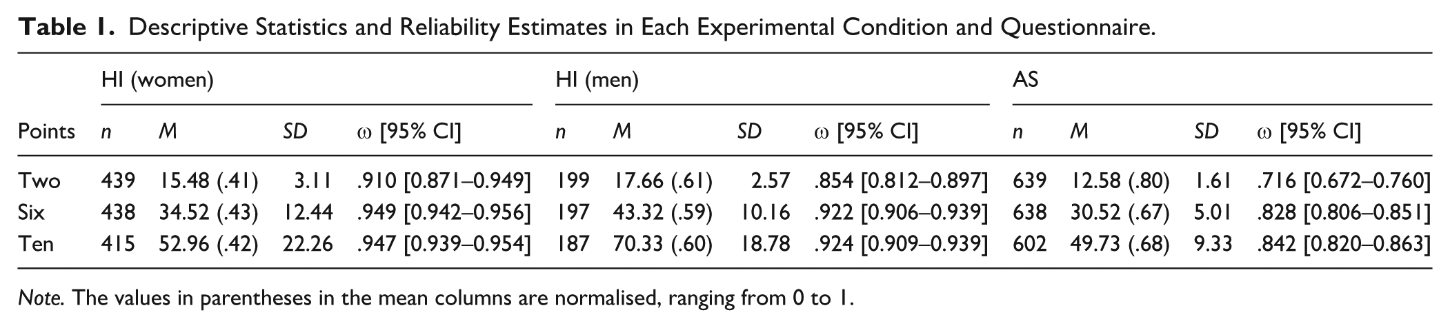
Note. The values in parentheses in the mean columns are normalised, ranging from 0 to 1.

Reliability

As expected, the reliability varied depending on the number of options (see Tables 1 and 2). We observed a statistically significant increase in reliability between the two- and six-point variants for AS, while no difference emerged between six- and 10-point variants. For HI, the same pattern was observed only in the men’s subsample. For women, two-point and six-point variants differed significantly. Combined χ² tests across questionnaires revealed that reliability increased from two to six options and then levelled off.

Table 2.

Differences in Internal Consistency (Using McDonald’s Omega) Between Two-, Six-, and 10-Point Scales.

Formats compared	HI (women)			HI (men)			AS			Combined
Formats compared	Δω	z	p	Δω	z	p	Δω	z	p	χ²	p
2–6	−.039	−1.97	.049	−.068	−3.34	<.001	−.112	−5.10	<.001	40.00	<.001
2–10	−.036	−1.84	.067	−.070	−3.31	<.001	−.126	−5.63	<.001	45.99	<.001
6–10	−.003	.700	.484	−.002	−.19	.846	−.014	−1.14	.253	1.83	.608

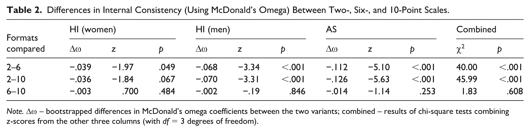
Note. Δω – bootstrapped differences in McDonald’s omega coefficients between the two variants; combined – results of chi-square tests combining z-scores from the other three columns (with df = 3 degrees of freedom).

Criterion Validity

The models had an excellent fit, and all variants had an equal relationship with the external criterion. Hence, the criterion validity seemed to hold for all the HI variants on the normalised sum score level. Although the differences between regression coefficients were observable, they were statistically negligible (see Table 3). However, after constraining all the residual covariances to the same value (model HI_cov), the model’s fit worsened rapidly, possibly because the six-point variant shared more residual variance with the 10-point than with the two-point scale. The effect was rather small (for men: r_2,6 = .736, r_2,10 = .667, r_6,10 = .846; for women: r_2,6 = .727, r_2,10 = .702, r_6,10 = .798 for the model HI_int). See Table 4 for correlations between the three HI variants and height.

Table 3.

Criterion Validity of Height Inventory (Both Men and Women).

							Model comparison					β
Mod.	χ²	df	p	TLI	RMSEA [90% CI]	SRMR	With	Δχ²	Δdf	Δp		2	6	10
HI_free											m:	.827	.872	.859
											w:	.878	.892	.887
HI_reg6,10	1.35	2	.510	1.001	0.000 [0.000–0.116]	.006	HI_free	1.35	2	.510	m:	.827	.870	.861
											w:	.878	.890	.889
HI_reg	3.45	4	.486	1.000	0.000 [0.000–0.095]	.011	HI_reg6,10	2.08	2	.354	m:	.838	.867	.858
											w:	.879	.890	.889
HI_var	9.49	8	.303	.999	0.036 [0.000–0.096]	.008	HI_reg	5.73	4	.220	m:	.850	.850	.850
											w:	.885	.885	.885
HI_int	11.21	12	.511	1.000	0.005 [0.000–0.070]	.009	HI_var	1.01	4	.908	m:	.850	.850	.850
											w:	.885	.885	.885
HI_cov	50.14	16	<.001	.990	0.103 [0.073–0.135]	.011	HI_int	38.64	4	<.001	m:	.853	.853	.853
											w:	.886	.886	.886

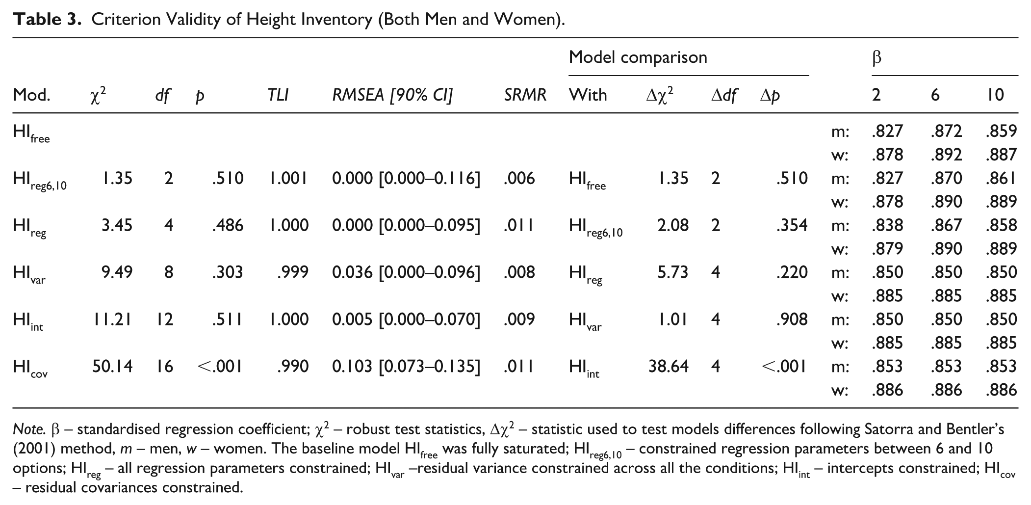
Note. β – standardised regression coefficient; χ² – robust test statistics, Δχ² – statistic used to test models differences following Satorra and Bentler’s (2001) method, m – men, w – women. The baseline model HI_free was fully saturated; HI_reg6,10 – constrained regression parameters between 6 and 10 options; HI_reg – all regression parameters constrained; HI_var –residual variance constrained across all the conditions; HI_int – intercepts constrained; HI_cov – residual covariances constrained.

Table 4.

Correlation Matrix of Height Inventory Variants and Real Height.

Variable	HI 2-point	HI 6-point	HI 10-point	Height
HI 2-point	1	0.930 [0.905, 0.948]	0.907 [0.875, 0.931]	0.839 [0.793, 0.876]
HI 6-point	0.945 [0.932, 0.955]	1	0.961 [0.946, 0.971]	0.876 [0.839, 0.905]
HI 10-point	0.938 [0.923, 0.950]	0.959 [0.949, 0.966]	1	0.869 [0.829, 0.900]
Height	0.883 [0.860, 0.902]	0.901 [0.882, 0.917]	0.897 [0.876, 0.914]	1

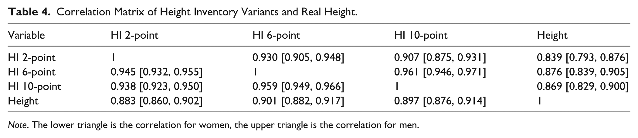
Note. The lower triangle is the correlation for women, the upper triangle is the correlation for men.

Measurement Models

Based on the TLI index, both HI (model HI_config) and AS (model AS_config) configural models had an excellent incremental fit (see Tables 5 and 6). However, RMSEA and SRMR for the HI were beyond acceptable values. After inspecting the residual covariance matrix, a systematic pattern was observed between inversed and non-inversed items, suggesting slight multidimensionality (with positive and negative factors), common with reversed-keyed items. We decided to neglect the effect, as it should not bias further analyses, though it still limited our results.

Table 5.

Measurement Invariance Testing of Experimental Conditions in Height Inventory (Women Only).

						Model comparison
Model	χ²	df	TLI	RMSEA [90% CI]	SRMR	With	Δχ²	Δdf	Δp
HI_config	2,443.8	458	0.974	0.086 [0.083–0.090]	0.092
HI_load	2,494.9	478	0.974	0.085 [0.082–0.088]	0.092	HI_config	9.73	20	.973
HI_metric	2,543.4	501	0.975	0.084 [0.080–0.087]	0.092	HI_thresh	19.31	23	.683
HI_scalar	2,579.5	521	0.976	0.082 [0.079–0.086]	0.092	HI_metric	13.43	20	.858
HI_strict	2,092.8	543	0.983	0.070 [0.067–0.073]	0.094	HI_scalar	13.51	22	.918
HI_lvmeans	2,082.4	545	0.983	0.070 [0.066–0.073]	0.094	HI_strict	.12	2	.940
HI_lvvar	2,405.2	548	0.979	0.076 [0.073–0.079]	0.106	HI_lvmeans	29.19	3	<.001
HI_lvcov	2,403.3	551	0.980	0.076 [0.073–0.079]	0.105	HI_lvvar	8.84	3	.031
HI_rescov	2,490.4	573	0.980	0.076 [0.073–0.079]	0.106	HI_lvcov	72.26	22	<.001

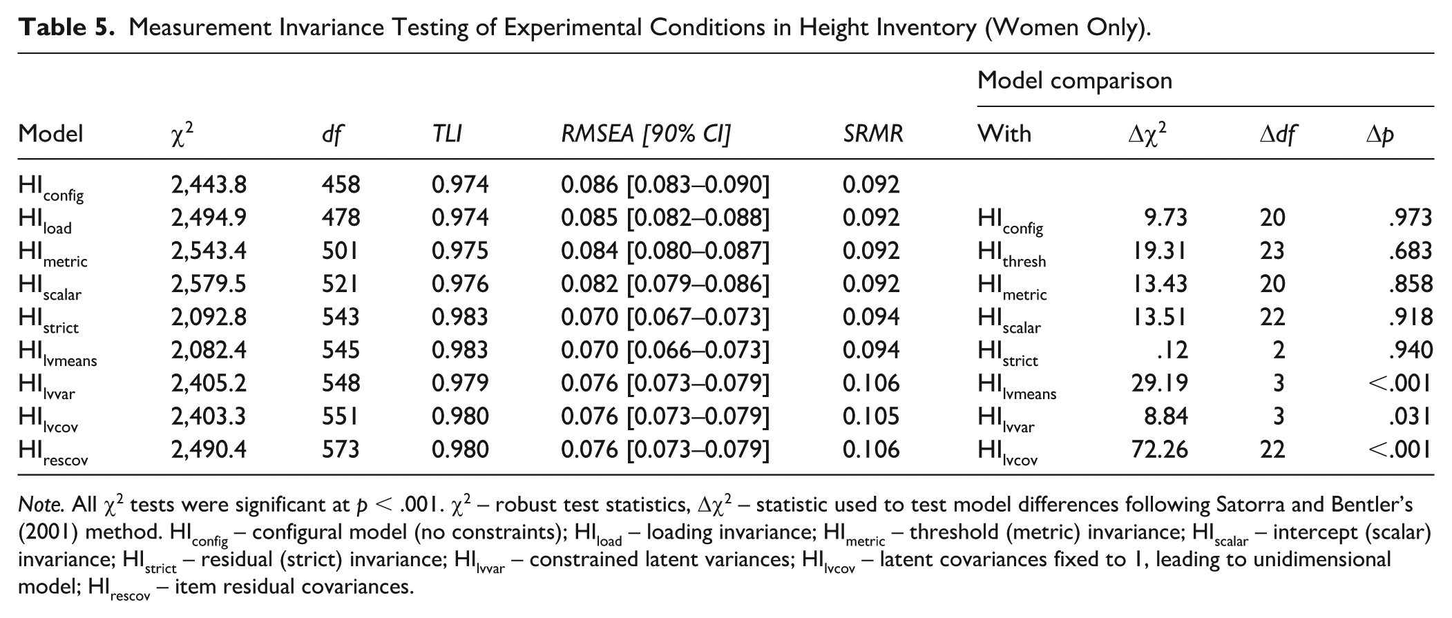
Note. All χ² tests were significant at p < .001. χ² – robust test statistics, Δχ² – statistic used to test model differences following Satorra and Bentler’s (2001) method. HI_config – configural model (no constraints); HI_load – loading invariance; HI_metric – threshold (metric) invariance; HI_scalar – intercept (scalar) invariance; HI_strict – residual (strict) invariance; HI_lvvar – constrained latent variances; HI_lvcov – latent covariances fixed to 1, leading to unidimensional model; HI_rescov – item residual covariances.

Table 6.

Measurement Invariance Testing of Experimental Conditions in the Autonomy Subscale.

						Model comparison
Model	χ²	df	TLI	RMSEA [90% CI]	SRMR	With	Δχ²	Δdf	Δp
AS_config	746.6	164	0.949	0.065 [0.060–0.070]	0.061
AS_load	759.3	176	0.952	0.063 [0.058–0.067]	0.061	AS_config	18.74	12	.095
AS_metric	774.5	191	0.956	0.060 [0.056–0.065]	0.061	AS_thresh	27.57	15	.024
AS_scalar	793.0	203	0.958	0.059 [0.054–0.063]	0.061	AS_metric	23.41	12	.024
AS_strict	669.6	217	0.970	0.050 [0.045–0.054]	0.063	AS_scalar	7.25	14	.925
AS_lvmeans	664.3	219	0.971	0.049 [0.045–0.053]	0.063	AS_strict	.14	2	.933
AS_lvvar	724.6	222	0.967	0.052 [0.048–0.056]	0.069	AS_lvmeans	15.99	3	.001
AS_lvcov	697.3	225	0.970	0.050 [0.046–0.054]	0.070	AS_lvvar	1.04	3	.792
AS_rescov	724.9	239	0.971	0.049 [0.045–0.053]	0.071	AS_lvcov	22.49	14	.069

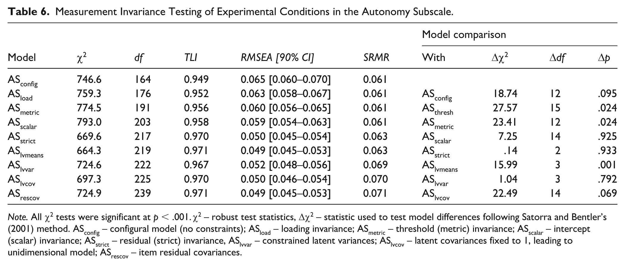
Note. All χ² tests were significant at p < .001. χ² – robust test statistics, Δχ² – statistic used to test model differences following Satorra and Bentler’s (2001) method. AS_config – configural model (no constraints); AS_load – loading invariance; AS_metric – threshold (metric) invariance; AS_scalar – intercept (scalar) invariance; AS_strict – residual (strict) invariance, AS_lvvar – constrained latent variances; AS_lvcov – latent covariances fixed to 1, leading to unidimensional model; AS_rescov – item residual covariances.

Measurement Invariance

In both HI and AS, we observed strict invariance. After constraining the latent variances, the chi-square difference (Δχ²) statistics were statistically significant for both measurement tools. Indeed, latent variance increased for the two-point format but not for longer variants, although this trend was apparent especially for the HI (for the HI, latent standard deviations were ψ_2-point = 1.74, ψ_6-point = 1.51, ψ_10-point = 1.45; for the AS ψ_2-point = 1.37; ψ_6-point = 1.32, ψ_10-point = 1.32). This suggests that with increasing response options, respondents tended to gravitate more towards middle options. The preference for middle options compared to more extreme ones was also evident after a graphical inspection of threshold parameter estimates (see Figures 1 and 2). Although the change after constraining latent variances was statistically significant, the changes in fit indices were still practically negligible. Interestingly, the model with latent covariances fixed to 1 also did not produce any statistically significant changes (for AS), supporting the underlying unidimensionality, which suggests that all variants measured the same attribute. We, therefore, concluded that the number of response categories influences only the raw score distribution and its reliability but not the measured latent trait.

Figure 1.

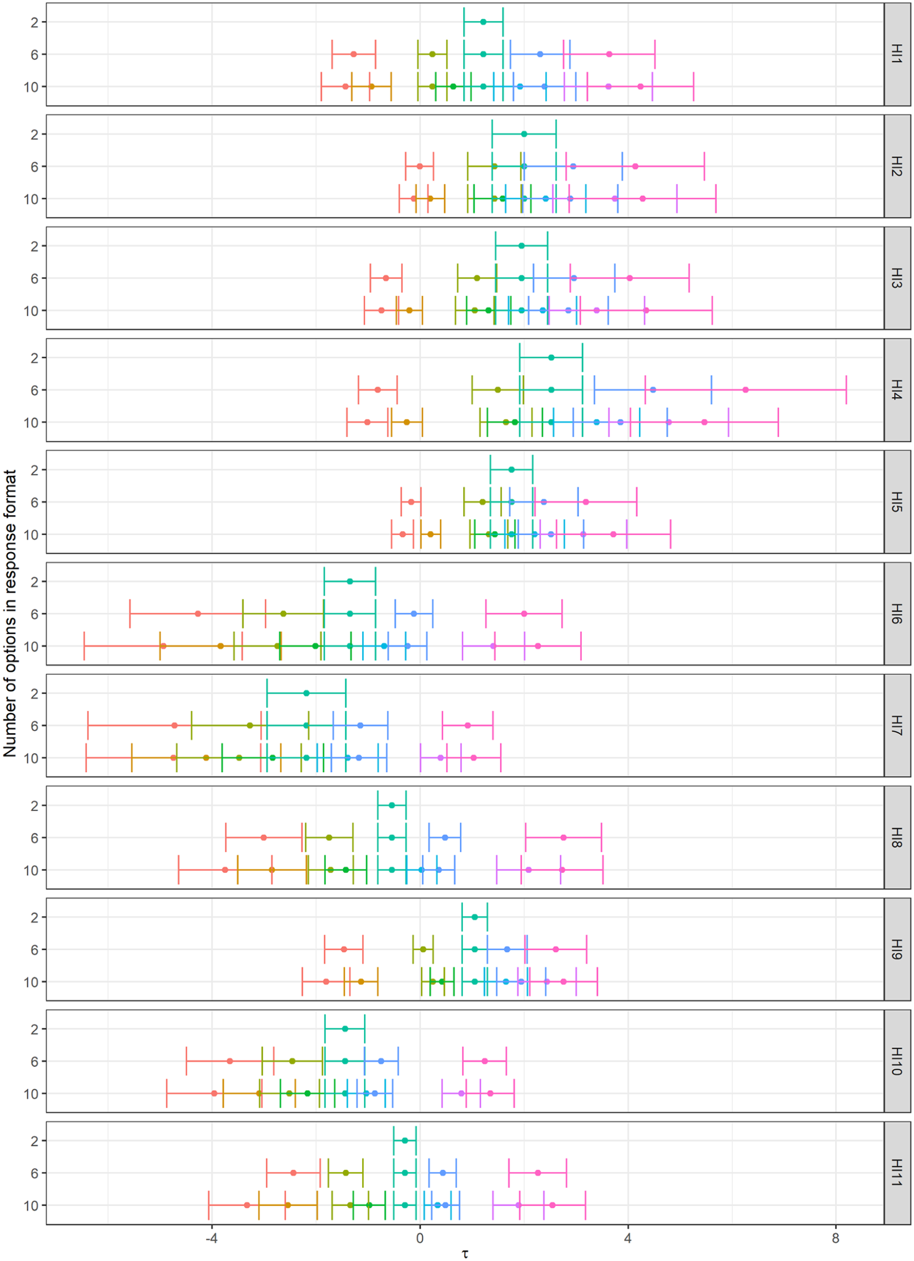
Unstandardised threshold estimates for HI (Model HI_load with fixed loadings).

Figure 2.

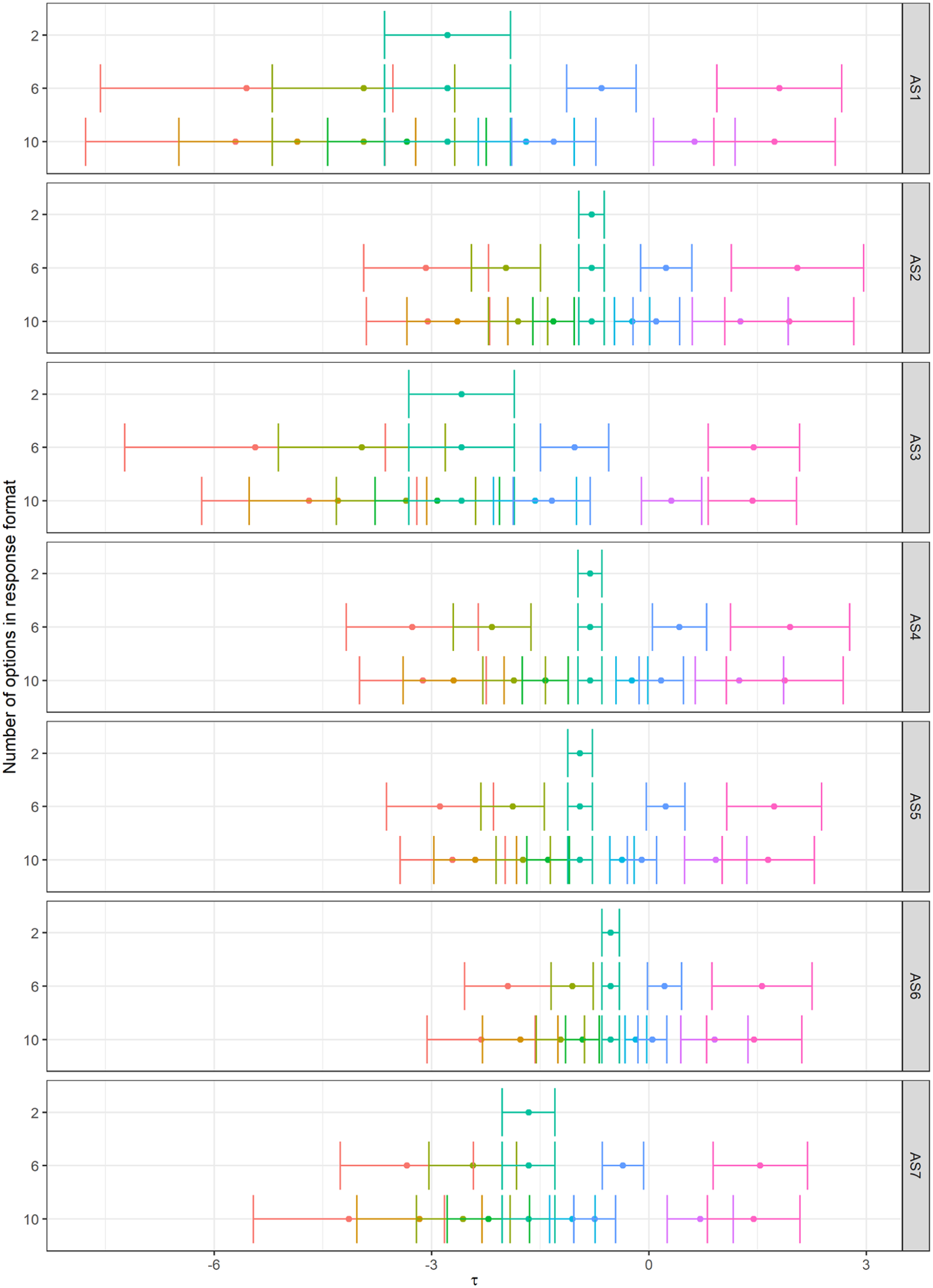
Unstandardised threshold estimates for AS (Model AS_load with fixed loadings).

The graphical examination revealed another interesting insight into respondents’ answers in response to increasing options. Specifically, odd-numbered thresholds were usually very close to either of the neighbouring thresholds in 10-point formats. However, since metric invariance yielded either non-significant results (the HI) or significant differences but with negligible changes in models’ fit (the AS), we assume this observation is also of little consequence.

Trait Criterion Validity

The initial, fully constrained unidimensional model HI_rescov had an acceptable fit to the data, see Table 7, except for the SRMR index (reasons discussed above). Releasing the parameters led to statistically significant improvements, but the fit indices remained unchanged (<.001). Overall, the criterion validity of the latent trait was the same in all experimental conditions, which aligns with the findings that all the variants are unidimensional. In other words, the number of options did not influence the strength of the linear relationship between the latent trait and the criterion.

Table 7.

Trait Criterion Validity for Height Inventory (Women Only).

						Model comparison				β
Model	χ²	df	TLI	RMSEA [90% CI]	SRMR	With	Δχ²	Δdf	Δp	2	6	10
HI_full	2,301.4	605	0.981	0.070 [0.067–0.073]	0.095					.830	.830	.830
HI_freecov	2,207.7	602	0.982	0.068 [0.065–0.071]	0.094	HI_full	21.17	3	<.001	.833	.833	.833
HI_freevar	2,221.7	599	0.981	0.068 [0.065–0.071]	0.093	HI_freecov	7.03	3	.071	.849	.903	.933
HI_freereg	2,193.4	597	0.982	0.068 [0.065–0.071]	0.093	HI_freevar	15.38	2	<.001	.915	.883	.892

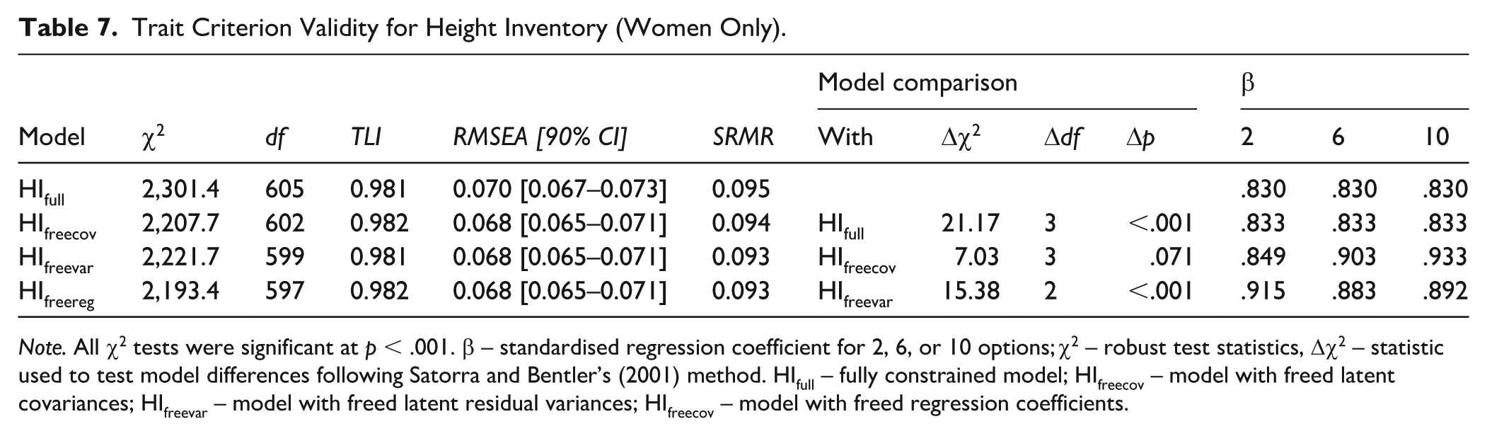
Note. All χ² tests were significant at p < .001. β – standardised regression coefficient for 2, 6, or 10 options; χ² – robust test statistics, Δχ² – statistic used to test model differences following Satorra and Bentler’s (2001) method. HI_full – fully constrained model; HI_freecov – model with freed latent covariances; HI_freevar – model with freed latent residual variances; HI_freecov – model with freed regression coefficients.

Discussion

The existing research on the number of response options in Likert-type response format has often focused on correlations with inadequate criteria, or it neglected the validity altogether, focusing solely on internal consistency and descriptive statistics. This study comprehensively examined all these aspects and bridged limitations using human height as the measured attribute. Moreover, we aimed to examine the influence of the methodological component (i.e., Likert-type response format) on the measurement model, another aspect often overlooked in the existing research (to our knowledge, only Xu and Leung (2018) examined this effect). Using a repeated-measure design, we manipulated the number of response options (two, six, and 10) in the Likert-type response format. This approach enabled us to separate various sources of variance and examine the methodological component stemming solely from differences in the Likert-type response format. We used a more formal approach than previous studies, including invariance testing and criterion validation at both manifest and latent levels. Furthermore, we demonstrated that our observation can be generalised to another construct in psychology.

Main Results Summary and Interpretation

Our results indicated that adding more options to the response format can lead to a shift towards the centre if the item is normalised to the same range (e.g., 0–1). This is an obvious consequence of the fact that with a binary scale, all the responses are extreme (i.e., 0 or 1), while more central responses can occur only with longer response formats. A significant difference in means was only found when comparing two- and six-point scales, while no difference was observed between six- and 10-point scales. This observation is consistent with Simms et al.’s (2019) study. The effect was strong in the case of the AS, while it was relatively small in the HI. We attribute this difference to AS being more skewed than HI. Overall, direct comparison of raw scores of different forms of the same questionnaire, varying in the number of response options, is limited, especially the comparison between the questionnaire with few (e.g., binary) versus many (e.g., six or more) response options. Following our results of invariance testing, more advanced equating options seem suitable (for example, the equipercentile method).

Regarding internal consistency, our results replicated the typical pattern in existing research, revealing that reliability increases with an increasing number of options in the Likert-type response format but levels off when reaching six options (Muñiz et al., 2005; Simms et al., 2019). Hence, the 10-point response format did not offer any meaningful additional information. However, the overall magnitude of differences in McDonald’s omega was relatively small, suggesting the differences between the two-point and longer variants are of little consequence.

Both shorter and longer variants explained the same portion of the variance in the criterion (here, respondents’ height). Thus, the correlation with the criterion did not follow the reliability pattern as expected if the increase in reliability was solely due to increased precision. Moreover, longer scales (with six and 10 response options) shared more construct-irrelevant variances, manifesting as higher residual covariances than covariances between two–six or two–10 options. The best explanation is that incorporating scales with more response options induces so-called method factors, that is, systematic variance unrelated to the measured latent trait, which increases internal consistency but not criterion validity. If this hypothesis is valid, using fewer (even binary) than more response options would help reduce the construct-irrelevant variance. Response formats with more points could positively bias correlations between raw scores across questionnaires, as they use the same response format burdened with the same method factors.

A closer examination of the internal structures of questionnaires and measurement invariance revealed that all variants had the same underlying measurement model and population parameters. Furthermore, all variants measured the same latent trait. Regarding the trait criterion validity for Height Inventory, at the latent level, all vaiants had the same relationship to the objective criterion. Although the hierarchical model comparison identified some significant differences, the changes in fit indices were negligible, suggesting no substantial differences between variants. Accordingly, using structural equation models (SEM) instead of raw score analysis could overcome any biases induced by response scale properties.

Strict measurement invariance across formats in the ordinal factor analysis did not contradict our proposition about the construct-irrelevant variance per se, which is still possible under certain conditions, especially if it is equally shared across items and if it does not influence items’ difficulties. The omega coefficient increased with more response options, clearly following Green and Yang’s (2009) threshold correction, increasing measurement stability and, thus, criterion validity. Simultaneously, the hidden, construct-irrelevant factor in longer forms may influence an exact position on the latent trait continuum, decreasing criterion validity. Both effects may counterbalance each other.

Unfortunately, such a situation should lower the criterion validity of latent traits, which was not observed. We assume our sample size was too small to observe the effect, which is likely when considering the variability in standardised regression parameters across models (see Table 7). Another explanation is the misfit of our measurement model, especially when considering SRMR and RMSEA indices, which may have concealed other important effects. Still, this fact limits our interpretation, and this pattern should be explored in more detail in future studies before a generalisation of our results is made.

Limitations

The longitudinal design resulted in a 40% dropout at the last measurement occasion. However, all experimental conditions were distributed equally across all measurement occasions, and the ratio of basic demographic characteristics was constant. Another major limitation was a smaller sample size, which forced us to omit men from some analyses due to the nature of some analytic procedures and may have led to the inability to detect some effects when testing trait criterion validity (as discussed above). Finally, we stress that our measurement model did not fit the data well, especially when evaluating SRMR and RMSEA indices. Reverse-coded items and the effects related to them were the main reasons; therefore, future research should address their correct incorporation into our design.

Further Research

First, more attention should be given to interactions between the number of response categories and other aspects of the Likert-type response format. Although some conclusions have been made about the interaction of the number of response options and verbal anchors (Hamby & Peterson, 2016), again, the focus was primarily on reliability, and a thorough validity assessment is still lacking. The importance of high-quality methodology (incorporating longitudinal, experimental, and within-subject design) cannot be stressed enough.

Second, future studies could “zoom into” the cognitive processes involved in responding to Likert-type items with different numbers of response categories and investigate why reliability increases and subsequently levels off. Working memory may play a role in the process of responding to an item, as this process is hypothesised to consist of several steps, including retrieval of relevant memories, the assessment of memories in relation to the item, and the selection of the best-fitting option (Tourangeau et al., 2000; Tourangeau & Rasinski, 1988). With an increasing number of options, choosing the degree of agreement or disagreement may become challenging, potentially leading to cognitive overload. Therefore, respondents may divide the response format to decrease cognitive overload. Another explanation may be directly related to Green and Yang’s (2009) correction. Using their equations, the relation between the number of options and the reliability could be derived analytically, which is beyond the scope of our paper.

Third, improving reliability while retaining the same criterion validity and measurement model of a scale with more response categories is essential. Criterion validity testing revealed higher residual covariances in longer scale variants, and method factors (i.e., systematic but construct-irrelevant sources) seemed to increase reliability. Thoroughly understanding this process and examining the influence of response styles and other sources of systematic bias could improve the validity of psychological measurement. While this study focused primarily on internal consistency, test–retest reliability was not addressed. Future research designs should be expanded to incorporate the estimation test–retest reliability in addition to internal consistency estimates, as emphasised in some sources (McCrae et al., 2011).

Finally, incorporating technologies (such as eye-tracking and mouse tracking) might help clarify the item-response process. Research designs should employ thinking-aloud protocols (Rigby et al., 2020) to understand the process better.

Conclusion

Although two-point variants significantly differed in means and reliability compared to six- and 10-point variants, the magnitude of the difference was relatively small. Moreover, all aspects of validity (criterion, measurement model, and trait criterion validity) remained unaffected. Hence, response formats with fewer response options can be routinely considered, especially in scales with more items. However, note that the specifics of the measured phenomena in question should be considered when choosing a response format.

Footnotes

Acknowledgements

The authors would like to thank Stanislav Ježek and Eva Šragová for their critical comments and insights.

ORCID iDs

Petra Hubatka

Hynek Cígler

David Elek

Ethical Considerations

The use of data in the current research project has been approved by the Research Ethics Committee of Masaryk University (EKV-2022-027).

Author Contributions

Conceptualization: P. Hubatka and H. Cígler; Methodology: P. Hubatka and H. Cígler; Investigation: P. Hubatka, Formal Analysis: D. Elek, H. Cígler, and P. Hubatka, Writing – Original Draft Preparation: P. Hubatka and H. Cígler, Writing – Review & Editing – P. Hubatka, H. Cígler, and D. Elek.

Funding

The authors disclosed receipt of the following financial support for the research, authorship, and/or publication of this article: This study was supported by the Czech Science Foundation (project number GA23-06924S).

Declaration of Conflicting Interests

The authors declared no potential conflicts of interest with respect to the research, authorship, and/or publication of this article.

Supplemental Material

Supplemental material for this article is available online in the OSF repository .

Data Availability Statement

The datasets and R code are publicly available in the OSF repository .

References

Bandalos

D. L.

Enders

C. K.

(1996). The effects of nonnormality and number of response categories on reliability. Applied Measurement in Education, 9(2), 151–160. https://doi.org/10.1207/s15324818ame0902_4

Bates

Mächler

Bolker

Walker

(2015). Fitting linear mixed-effects models using lme4. Journal of Statistical Software, 67(1), 1–48. https://doi.org/10.18637/jss.v067.i01

Bendig

A. W.

(1953). The reliability of self-ratings as a function of the amount of verbal anchoring and of the number of categories on the scale. Journal of Applied Psychology, 37(1), 38–41. https://doi.org/10.1037/h0057911

Borsboom

Mellenbergh

G. J.

Van Heerden

(2002). Different kinds of DIF: A distinction between absolute and relative forms of measurement invariance and bias. Applied Psychological Measurement, 26(4), 433–450. https://doi.org/10.1177/014662102237798

Chang

(1994). A psychometric evaluation of 4-point and 6-point Likert-type scales in relation to reliability and validity. Applied Psychological Measurement, 18(3), 205–215. https://doi.org/10.1177/014662169401800302

Chen

F. F.

(2007). Sensitivity of goodness of fit indexes to lack of measurement invariance. Structural Equation Modeling: A Multidisciplinary Journal, 14(3), 464–504. https://doi.org/10.1080/10705510701301834

Cheung

G. W.

Rensvold

R. B.

(2002). Evaluating goodness-of-fit indexes for testing measurement invariance. Structural Equation Modeling: A Multidisciplinary Journal, 9(2), 233–255. https://doi.org/10.1207/S15328007SEM0902_5

Cox

Pant

Gilson

A. N.

Rodriguez

J. L.

Young

K. R.

Kwon

Weed

N. C.

(2012). Effects of augmenting response options on MMPI–2 RC scale psychometrics. Journal of Personality Assessment, 94(6), 613–619. https://doi.org/10.1080/00223891.2012.700464

Deci

E. L.

Ryan

R. M.

(1985). Intrinsic motivation and self-determination in human behavior. Springer. https://doi.org/10.1007/978-1-4899-2271-7

10.

Fox

Weisberg

(2019). An R companion to applied regression (3rd ed.). Sage. https://socialsciences.mcmaster.ca/jfox/Books/Companion/

11.

Gagné

(2003). The role of autonomy support and autonomy orientation in prosocial behavior engagement. Motivation and Emotion, 27(3), 199–223. https://doi.org/10.1023/A:1025007614869

12.

Green

S. B.

Yang

(2009). Reliability of summed item scores using structural equation modeling: An alternative to coefficient alpha. Psychometrika, 74(1), 155–167. https://doi.org/10.1007/s11336-008-9099-3

13.

Hamby

Peterson

R. A.

(2016). A meta-analytic investigation of the relationship between scale-item length, label format, and reliability. Methodology, 12(3), 89–96. https://doi.org/10.1027/1614-2241/a000112

14.

Hilbert

Küchenhoff

Sarubin

Nakagawa

T. T.

Bühner

(2015). The influence of the response format in a personality questionnaire: An analysis of a dichotomous, a Likert-type, and a visual analogue scale. Testing, Psychometrics, Methodology in Applied Psychology, 23(1), 3–24. https://doi.org/10.4473/TPM23.1.1

15.

Jacoby

Matell

M. S.

(1971). Three-point Likert scales are good enough. Journal of Marketing Research, 8(4), 495–500. https://doi.org/10.1177/002224377100800414

16.

Ježek

Macek

Bouša

(2016). Cesty k nezávislosti: Jak se vyvíjí autonomie s identitou [Path to independency: Autonomy and identity development]. In Lacinová

Ježek

Macek

(Eds.), Cesty do dospělosti: Psychologické a sociální charakteristiky dnešních dvacátníků [Paths to Adulthood: Psychological and Social Characteristics of Current Vicenarians] (pp. 25–39). Masarykova univerzita.

17.

Johnston

M. M.

Finney

S. J.

(2010). Measuring basic needs satisfaction: Evaluating previous research and conducting new psychometric evaluations of the Basic Needs Satisfaction in General Scale. Contemporary Educational Psychology, 35(4), 280–296. https://doi.org/10.1016/j.cedpsych.2010.04.003

18.

Jones

W. P.

Loe

S. A.

(2013). Optimal number of questionnaire response categories: More may not be better. SAGE Open, 3(2), 215824401348969. https://doi.org/10.1177/2158244013489691

19.

Jorgensen

T. D.

Pornprasertmanit

Schoemann

A. M.

Rosseel

(2022). semTools: Useful tools for structural equation modeling (Version R package version 0.5-6.) [Computer software]. https://CRAN.R-project.org/package=semTools

20.

Kam

C. C. S.

Meyer

J. P.

Sun

(2021). Why do people agree with both regular and reversed items? A logical response perspective. Assessment, 28(4), 1110–1124. https://doi.org/10.1177/10731911211001931

21.

Kelley

(2007). Confidence intervals for standardized effect sizes: Theory, application, and implementation. Journal of Statistical Software, 20(8), 1–24. https://doi.org/10.18637/jss.v020.i08

22.

Lee

Paek

(2014). In search of the optimal number of response categories in a rating scale. Journal of Psychoeducational Assessment, 32(7), 663–673. https://doi.org/10.1177/0734282914522200

23.

Leung

S.-O.

(2011). A comparison of psychometric properties and normality in 4-, 5-, 6-, and 11-point Likert scales. Journal of Social Service Research, 37(4), 412–421. https://doi.org/10.1080/01488376.2011.580697

24.

C.-H.

(2016). The performance of ML, DWLS, and ULS estimation with robust corrections in structural equation models with ordinal variables. Psychological Methods, 21(3), 369–387. https://doi.org/10.1037/met0000093

25.

Likert

(1932). A technique for the measurement of attitudes. Archieves of Psychology, 22(140), 5–55.

26.

Lozano

L. M.

García-Cueto

Muñiz

(2008). Effect of the number of response categories on the reliability and validity of rating scales. Methodology, 4(2), 73–79. https://doi.org/10.1027/1614-2241.4.2.73

27.

Lüdecke

(2018). sjstats: Statistical functions for regression models (Version 0.17.2) [Computer software]. Zenodo. https://doi.org/10.5281/ZENODO.1284472

28.

Martinková

Drabinová

(2019). ShinyItemAnalysis for teaching psychometrics and to enforce routine analysis of educational tests. The R Journal, 10(2), 503. https://doi.org/10.32614/RJ-2018-074

29.

McCrae

R. R.

Kurtz

J. E.

Yamagata

Terracciano

(2011). Internal consistency, retest reliability, and their implications for personality scale validity. Personality and Social Psychology Review, 15(1), 28–50. https://doi.org/10.1177/1088868310366253

30.

Muñiz

Garcı́a-Cueto

Lozano

L. M.

(2005). Item format and the psychometric properties of the Eysenck Personality Questionnaire. Personality and Individual Differences, 38(1), 61–69. https://doi.org/10.1016/j.paid.2004.03.021

31.

Nadler

J. T.

Weston

Voyles

E. C.

(2015). Stuck in the middle: The use and interpretation of mid-points in items on questionnaires. The Journal of General Psychology, 142(2), 71–89. https://doi.org/10.1080/00221309.2014.994590

32.

Preston

C. C.

Colman

A. M.

(2000). Optimal number of response categories in rating scales: Reliability, validity, discriminating power, and respondent preferences. Acta Psychologica, 104(1), 1–15. https://doi.org/10.1016/S0001-6918(99)00050-5

33.

Putnick

D. L.

Bornstein

M. H.

(2016). Measurement invariance conventions and reporting: The state of the art and future directions for psychological research. Developmental Review, 41, 71–90. https://doi.org/10.1016/j.dr.2016.06.004

34.

R Core Team. (2021). R: A language and environment for statistical computing [Computer software]. R Foundation for Statistical Computing. https://www.R-project.org/

35.

Rečka

(2018). Dotazník výšky a váhy [Questionnaire of height and weight] [Master’s thesis]. Masarykova univerzita. https://is.muni.cz/th/ug7c2/Recka_Diplomova_prace.pdf

36.

Revelle

(2024). psych: Procedures for psychological, psychometric, and personality research (Version R package version 2.4.1) [Computer software]. Northwestern University. https://CRAN.R-project.org/package=psych

37.

Rigby

Vass

Payne

(2020). Opening the ‘black box’: An overview of methods to investigate the decision-making process in choice-based surveys. The Patient–Patient-Centered Outcomes Research, 13(1), 31–41. https://doi.org/10.1007/s40271-019-00385-8

38.

Rosseel

(2012). lavaan: An R package for structural equation modeling. Journal of Statistical Software, 48(2), 1–36. https://doi.org/10.18637/jss.v048.i02

39.

Ryan

R. M.

Deci

E. L.

(2000). Self-determination theory and the facilitation of intrinsic motivation, social development, and well-being. American Psychologist, 55(1), 68–78. https://doi.org/10.1037/0003-066X.55.1.68

40.

Sass

D. A.

Schmitt

T. A.

Marsh

H. W.

(2014). Evaluating model fit with ordered categorical data within a measurement invariance framework: A comparison of estimators. Structural Equation Modeling: A Multidisciplinary Journal, 21(2), 167–180. https://doi.org/10.1080/10705511.2014.882658

41.

Satorra

Bentler

P. M.

(2001). A scaled difference chi-square test statistic for moment structure analysis. Psychometrika, 66(4), 507–514. https://doi.org/10.1007/BF02296192

42.

Sijtsma

(2009). On the use, the misuse, and the very limited usefulness of Cronbach’s alpha. Psychometrika, 74(1), 107–120. https://doi.org/10.1007/s11336-008-9101-0

43.

Sijtsma

Pfadt

J. M.

(2021a). Part II: On the use, the misuse, and the very limited usefulness of Cronbach’s alpha: Discussing lower bounds and correlated errors. Psychometrika, 86(4), 843–860. https://doi.org/10.1007/s11336-021-09789-8

44.

Sijtsma

Pfadt

J. M.

(2021b). Rejoinder: The future of reliability. Psychometrika, 86(4), 887–892. https://doi.org/10.1007/s11336-021-09807-9

45.

Simms

L. J.

Zelazny

Williams

T. F.

Bernstein

(2019). Does the number of response options matter? Psychometric perspectives using personality questionnaire data. Psychological Assessment, 31(4), 557–566. https://doi.org/10.1037/pas0000648

46.

Torchiano

(2020). effsize: Efficient effect size computation (Version R package version 0.8.1) [Computer software]. Zenodo. https://doi.org/10.5281/ZENODO.1480624

47.

Tourangeau

Rasinski

K. A.

(1988). Cognitive processes underlying context effects in attitude measurement. Psychological Bulletin, 103(3), 299–314. https://doi.org/10.1037/0033-2909.103.3.299

48.

Tourangeau

Rips

L. J.

Rasinski

(2000). The psychology of survey response. Cambridge University Press. https://doi.org/10.1017/CBO9780511819322

49.

Weijters

Cabooter

Schillewaert

(2010). The effect of rating scale format on response styles: The number of response categories and response category labels. International Journal of Research in Marketing, 27(3), 236–247. https://doi.org/10.1016/j.ijresmar.2010.02.004

50.

Weng

L.-J.

(2004). Impact of the number of response categories and anchor labels on coefficient alpha and test-retest reliability. Educational and Psychological Measurement, 64(6), 956–972. https://doi.org/10.1177/0013164404268674

51.

Wickham

(2016). ggplot2: Elegant graphics for data analysis [Computer software]. Springer-Verlag. https://ggplot2.tidyverse.org

52.

Estabrook

(2016). Identification of confirmatory factor analysis models of different levels of invariance for ordered categorical outcomes. Psychometrika, 81(4), 1014–1045. https://doi.org/10.1007/s11336-016-9506-0

53.

M. L.

Leung

S. O.

(2018). Effects of varying numbers of Likert scale points on factor structure of the Rosenberg Self-Esteem Scale. Asian Journal of Social Psychology, 21(3), 119–128. https://doi.org/10.1111/ajsp.12214