A two-stage method for damage detection using frequency responses and statistical theory

Abstract

In order to precisely identify the location and extent of structural damage, a two-stage damage detection method using frequency responses and statistical theory is presented in this paper. First, a damage index, which comes from the product of the stiffness changes and measured responses, is proposed. We can utilize degree-of-freedom (d.f.) damage index to localize the damage locations. Then, in order to calculate the extent of damage, a damage quantification formula is deduced from a reduced degree-of-freedom system. Finally, the effect of measurement noise is taken into account in the identification process and the measurement noise sensitivity formula based on statistical theory is presented. The numerical example and analysis demonstrate the excellent performance of the proposed two-stage method to identify damage locations and extent compared with other methods, such as the directness generalized inverse method.

Keywords

Damage detection degree-of-freedom frequency response harmonic excitation noise

1. Introduction

All engineering structures often accumulate damage during their service life. Existence of structural damage leads to modifications of the dynamic characteristics. These modifications are manifested as changes in the vibration parameters (natural frequencies, mode shapes, frequency responses etc.) which can be obtained from the results of dynamic testing. During the past two decades, many research works have been conducted in the area of damage detection based on vibration characteristics with different algorithms. One of the strategies is to use the measured frequency to detect structural damage (Dong et al., 2002; Hearn and Testa, 1991; Salawu, 1997). However, the measured modal frequencies are often limited and are not sensitive to local damage. Another strategy is to use the measured mode shape to detect structural damage (Guo and Zhang, 2006; Law et al., 1998; Shi et al., 2000a). These methods need to obtain modal frequencies and mode shapes by using modal identification techniques. Modal identification can be a time-consuming task and the curve fitting process itself always adds some unavoidable errors. Moreover, we lose a lot of information by using mode shapes. Therefore, the direct use of measured raw data for damage detection (e.g. in the form of frequency response data), may in most cases represent a considerable advantage (Maia et al., 2003).

Schulz and Naser (1998) presented a frequency response reference function method to detect damage. The method first uses measured frequency response functions (FRFs) of a healthy structure as reference data, and then computes cross-spectral densities between pairs of combined damage and external forces to identify any occurring damage. Maia et al. (2003) proposed some simple methods and tools, which are based on the use of frequency response functions, to detect damage. And the proposed FRF-based method is based on the assumption that damage is located at the point where the change of an operational mode shape function is the greatest. Zheng et al. (2001) utilizes the change of curvature of FRFs to identify thesingle damage problem. Zimmerman et al. (1995) and Park G et al. (2000) have also studied damage detection by using frequency response functions. If the measurement errors aren’t considered, these methods are often effective, especially to single damage problem. However, when the measurement errors are considered, it is difficult for these methods to identify damage locations and extent. Park and Park (2003) presented a method to identify damage locations using a reduced dynamic system and incompletely measured frequency response functions. The method considers the influence of measured noise, but it is difficult to identify damage extent. In order to solve these problems, it is desirable to develop a new method to identify damage locations and extent and to reduce the influence of measured noise.

In this paper a two-stage method is presented to identify damage locations and extent by directly using measured frequency response data. First, a damage index, which comes from the product of the stiffness changes and measured responses, is proposed. We can utilize degree-of-freedom (d.f.) damage index to localize the damage locations. Then, a damage quantification formula is deduced from a reduced d.f. system to calculate damage extent. Finally, the effect of measurement noise is taken into account in the identification process and the measurement noise sensitivity formula based on statistical theory is presented. It will be demonstrated that the proposed approach is effective. This paper is organized as follows: the basic theory is briefly introduced (Section 2). In Section 3, the two-stage method is presented and the measurement noise sensitivity formula based on statistical theory is analyzed. In Section 4, the directness generalized inverse method is briefly introduced and its noise sensitivity formula is analyzed. Numerical examples are given in Section 5. Finally, the paper is concluded in Section 6.

2. Basic equations

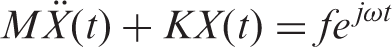
Consider an n-dimensional dynamic structure that is subjected to a forced harmonic excitation. The equation of motion can be expressed as

(1)

in which M, C, and K are the n × nmass, damping and stiffness matrices of the structure; X(t) represents the output or response vector; f is the vector of forcing amplitudes; j is the imaginary unit; and ω is the excitation frequency. Both X(t) and f are of length n. For general structures, some harmonic vibration exciters or vibration excitation devices can be employed to excite the structures and generate the forced harmonic excitation. The objective of this paper is to identify the location and extent of structural damage which is related to the stiffness matrix. The stiffness changes are small and would not cause a change in the connectivity of the structure. The proposed method would be applicable to a lightly damped structure where stiffness changes would not significantly affect the damping property of the structure. Therefore, the damping matrix is neglected even though damping reduces the modal frequency. Thus, equation (1) becomes

(2)

In general, structural damage refers to changes in the stiffness properties of the structure with no change in the mass property. The equation of motion with damage under the same excitation can be written as

(3)

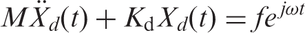
In which K_d is the stiffness matrix with damage; X_d (t) represents response vector with damage. The stiffness matrix and response vector of the structure with damage can be represented by

(4a)

(4b)

In which δK and δX are small change in the stiffness matrix and the response vector due to the damage, respectively.

Substituting equation (4) into (3) and noting (2), one gets

(5)

Because the input is harmonic, the steady-state output will also be harmonic. Thus, at steady state

(6a,b,c)

In which Y, δY and Y_d are the steady-state vibration amplitudes of X(t), δX(t) and X_d (t), respectively. Substituting equation (6) into (5), one obtains

(7)

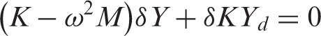
Equation (7) is strictly valid for a specific excitation frequency ω.

3. Two-stage damage identification method and sensitivity analysis of measured noise

3.1. Damage Localization

Here, a damage index will be proposed to identify structural damage sites. Consider equation (7), we have

(8)

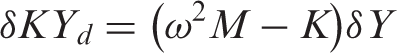
The right-hand side of equation (8) can be mainly determined from the change of measured frequency response data of undamaged and damaged structure. On the other hand, the left-hand side of the equation contains an unidentified term δK, which comes from damage. Thus, the δKY_d can be treated as a damage index to indicate the damage locations. Introducing a new variable η as the damage index, the damage index can be defined as

(9)

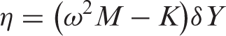
In which η is the n × 1 damage index variable. The damage of an element can cause the change of damage index of correlative degrees of freedom. Therefore, damage sites can be localized by using the damage index of different degrees of freedom.

3.2. Damage Quantification

After the damage sites have been preliminarily identified, the damage extent of the suspected damage elements should be determined. For a structure, the total number of elements is NE and the number of d.f. is n. Damage in the structure is assumed as stiffness reductions and its location is specified by the element number. If ND suspected damage elements have been identified in the NE elements, we only need determine the damage extent of the ND suspected damage elements.

It is difficult to model the damage in sufficient details for a general type of damage. Here, it is assumed that the reduction of structural stiffness due to damage as the summation of each elemental stiffness matrix multiplied by a damage coefficient (Shi, et al., 2000b), δK can be expressed as

(10)

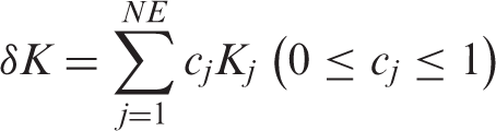
In which K_j and c_j are the jth elemental stiffness matrix and its damage coefficient, respectively; NE is the number of elements.

If ND suspected damage elements have been identified, the location vector of the ND suspected damage elements is R. Thus, equation (10) becomes

(11)

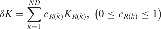
In which K_R(k) and c_R(k) are the R(k)th elemental stiffness matrix and its damage coefficient, respectively. Forexample, if the 2nd and 5th elements have been identified as the suspected damage elements, the number of suspected damage elements ND = 2 and the location vector R = {2,5}. So, K_R(1) = K₂, c_R(1) = c₂, express the 2nd elemental stiffness matrix and its damage coefficient. Similarly, K_R(2) = K₅, c_R(2) = c₅, express the 5th elemental stiffness matrix and its damage coefficient. Substituting equation (11) into (8), we have

(12)

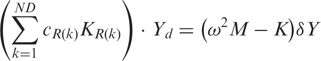
Now we proposed a d.f. reduction method to calculate damage extent. Actually, equation (12) is an n-dimensional system of equations. We first select ND degrees of freedom as reduced d.f. in the n degrees offreedom, and the ND degrees of freedom should be related to the ND suspected damage elements. And it is necessary that one degree of freedom should correlate with one suspected damage elements according to oneto one corresponding principle. 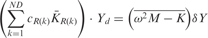Then, in the n-d.f elemental stiffness matrix K_R(k) we choose and get aND-d.f elemental stiffness matrix ${\bar{K}}_{R (k)}$ by using thereduced d.f.. The ${\bar{K}}_{R (k)}$ is a ND × n matrix. Similarly, From the n-d.f. matrix (ω²M − K) we choose and get a ND-d.f. matrix $\bar{(ω^{2} M - K)}$ . The $\bar{(ω^{2} M - K)}$ is also a ND × n matrix. So, the equation (12) can be written as

(13)

The d.f. number of equation (13) is ND. The left-hand side of equation (13) can be adjusted and the damage vector can be extracted:

(14)

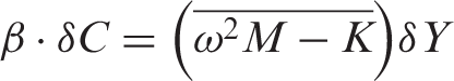
In which β is a ND × ND matrix, whose basic component can be expressed as 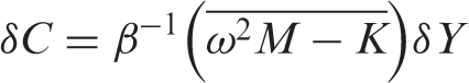$β_{m s} = \sum_{i = 1}^{n} {({\bar{K}}_{R (s)})}_{m i} \cdot {(Y_{d})}_{i}; δ C$ is the damage coefficient vector of the ND suspected damage elements. Therefore, equation (14) is a ND-dimensional system of equations. We can directly utilize the inverse of the matrix β to calculate the damage coefficient vector.

(15)

3.3. Measurement Noise and Sensitivity Analysis

For damage identification, the effects of measurement noise should be considered. The most realistic method would be to perform the test over and over again on the same structure under different conditions and compare the results of the different tests. This would be an expensive procedure. So, a more practical method would be to add artificial noise. According to literature (Ren and Roeck, 2002), in the numerical examples, noise is simulated by adding a series of pseudorandom numbers on the theoretically calculated responses. And the random numbers are originally generated from a uniform distribution on the interval [0,1], and then transformed to new random numbers on the interval [−1,1]. In general, the first time measured noise data will be used to identify damage. However, the noise is random. If we repeat to acquire the response data with random noise, the acquired noise data should be different from the previous noise data. This will lead to the change of identification results. Therefore, statistical theory is proposed to analyze the effects of random noise. And it is assumed that the undamaged model can be accurately acquired for the sake of convenience. Then, we will analyze the sensitivity of the damage index and damage coefficient with respect to noise on a frequency response. Consider equation (9) and equation (15), we have

(16)

(17)

(18)

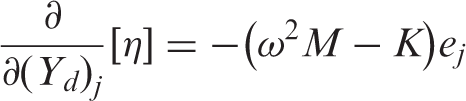
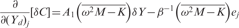
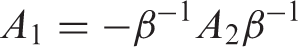
In which A₂ is a ND × ND matrix, whose basic component can be expressed as ${(A_{2})}_{m s} = {({\bar{K}}_{s})}_{m j}$ ; (Y_d)_j express the jth component of the vector Y_d; e_j is an n × 1 vector with a one in the jth element and zeros at all remaining elements. The random noise perturbation of Y_d is expressed as ΔY_d. The linear approximation to the change in the hth component of damage index and damage coefficient is

(19)

(20)

According to the literature (Ren and Roeck, 2002), it can be assumed the ΔY_d is a zero mean random variable uniformly distributed in an area. Thus, the ΔY_d can be expressed as Y_d α u. α is the noise level. u is a zero mean random variable uniformly distributed on the interval [−1,1]. So, the expected values of damage index η and damage coefficient δC are zero, i.e. E[Δη_h] = 0, E[Δ(δC_h)] = 0. The second central moment, or variance, is given as

(21)

(22)

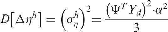
We can calculate all variances of damage index and damage coefficient in turn. The positive square root of the variance is the standard deviation of the quantity. Thus, from the standard variance we can know the noise sensitivity of the damage index and damage coefficient.

4. Sensitivity analysis of directness generalized inverse (DGI) method

The damage detection methods using frequency response also include the directness generalized inverse method (Dong et al., 2002). This method can simultaneously identify the location and extent of damage. We will simply describe the directness generalized inverse method and analyze the sensitivity of the method. Consider equation (8). Substituting equation (10) into (8) and noting P = (ω²M − K)δY, one gets

(23)

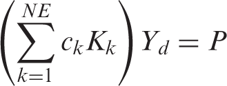
The left-hand side of equation (23) can be adjusted and the damage vector can be extracted, so we get

(24)

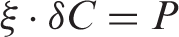
In which ξ is a n × NE matrix, whose basic component can be expressed as $ξ_{m s} = \sum_{i = 1}^{n} {(K_{s})}_{m i} \cdot {(Y_{d})}_{i}$ . The δC is the damage coefficient vector of the all NE elements. In general, the number n and the number NE are unequal. So we can utilize the Moore-Penrose generalized inverse (Norman, 1976) to solve this problem. We can get

(25)

An approximative sensitivity analysis of the directness generalized inverse method can be described as follows.

(26)

(27)

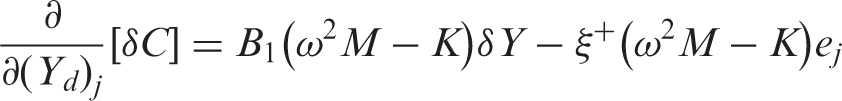
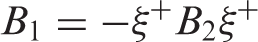
In which B₂ is a n × NE matrix, whose basic component can be expressed as (B²) = (K^s)_mj. Thus,

(28)

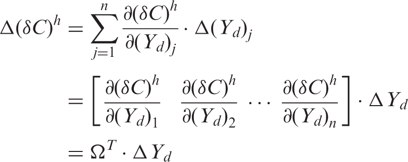
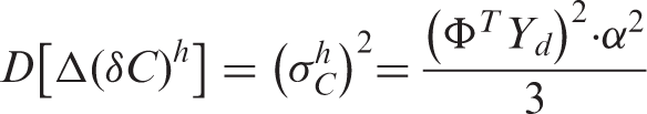
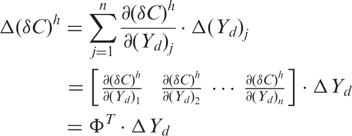
Similarly, ΔY_d can be expressed as Y_d α u; α is the noise level and u is a zero mean random variable uniformly distributed on the interval [−1,1]. The expected values of damage coefficient δC are zero. The variance of the hth component of δC is given as

(29)

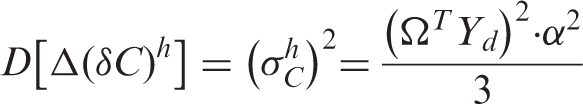
The positive square root of the variance is the standard variance. Thus, from the standard variance we can know the noise sensitivity of the damage coefficient.

5. Numerical examples

A two-dimensional truss structure is considered to demonstrate the process of damage detection (see Figure 1). In thetruss structure, E = 72 GPa, ρ = 2800 kg/m³, and A = 0.001m². The length of the truss structure is shown in Figure 1. The finite-element model of the truss consists of 30 rod elements, 14 nodes, and 24-d.f‥ Two damage cases are assumed with a reduction in the stiffness of individual bars in the structure. Case 1 has 20% reduction in the stiffness in element 10. Case 2 has 20% and 25% reduction in elements 9 and 21, respectively. Excitation force should be exerted on the free end of the truss structure. Therefore, a single harmonic force is applied to the right end of the structure, and the excited location is in the vertical direction of node 8. In general, selected excitation frequencies should be far away from the natural frequencies of the structure. Here, the excitation frequency is 2000 rad/s. we used the acquired frequency responses to identify damage.

Figure 1.

Two-dimensional truss structure.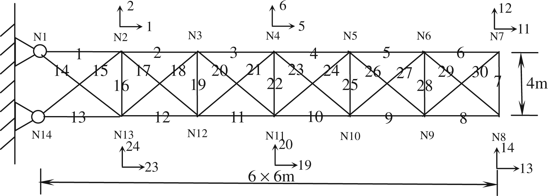

5.1. Case 1

In case 1, damage occurs in element 10 with 20% stiffness reduction. The two-stage damage identification method and the directness generalized inverse method were studied in this case. Great emphasis was also put on examining the influence of the measured noises on the accuracy of predicting the damage locations and extent.

The results of numerical calculations of the directness generalized inverse method are shown in Figure 2, where it can be seen that the damage occurs in element 10 and the damage extent is 0.1888. So, the identification results are very close to the true damage.

Figure 2.

Identification result of directness generalized inverse method when damage occurs in the 10th element.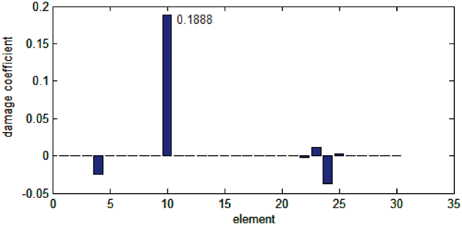

The measurement noise should be considered. Here, the measurement noise is simulated according to the literature (Ren and Roeck, 2002). Then, the variances of damage coefficient can be calculated according to equation (29). In this case, the noise level is 0.02. The computed results of the directness generalized inverse method with noise are shown in Figure 3. We can observe the damage coefficients of the perturbations along with ±1σ error bars. Thus, we can use the standard variance ±1σ to analyze the effects of the measurement noise. From Figure 3 it can be observed that the effects of the measurement noise far exceed the true damage. Thus, when the noise level is 0.02, the directness generalized inverse method cannot identify the true damage locations and extent.

Figure 3.

Identification result of directness generalized inverse method with noise when damage occurs in the 10th element (noise level 0.02, damage coefficients of the perturbations along with ±1σ error bars.).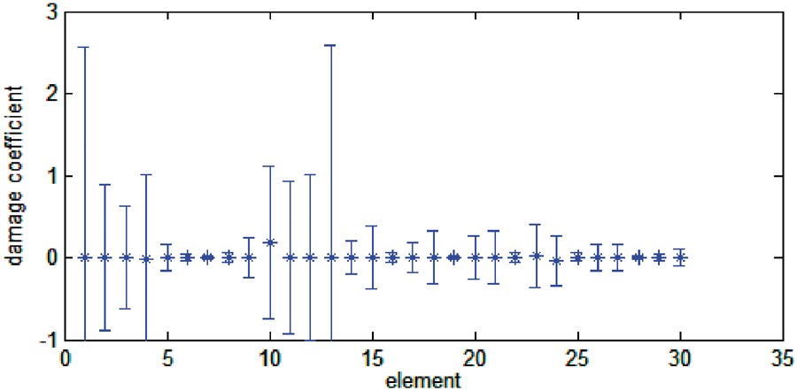

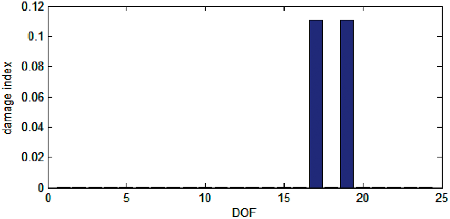
The proposed two-stage damage identification method was applied to identify damage. First, it is necessary to analyze damage location by using damage index. The computed results of damage localization are shown in Figure 4, where it can be observed that the changes of damage index occur in the d.f. 17 and 19. From Figure 1 it can be seen that element 10 is related to the d.f. 17 and 19. So, element 10 should be the suspected damage elements. Thus, the number of suspected damage elements ND = 1. We only need to select one d.f. to detect damage extent, and we just request that one selected d.f. should correspond to one damaged element. Here, we select d.f. 17 as the reduced d.f‥ Then, we use equation (14) and (15) to calculate the damage extent. From equation (14), we can get a simple equation. From equation (15) we can solve the simple equation and obtain the damage coefficient. The computed damage coefficient is shown as follows:

Figure 4.

Damage index of the two-stage method when damage occurs in the 10th element.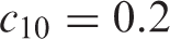

The identification result is equal to the true damage extent.

For the two-stage damage identification method, the measurement noise should also be considered. Here, the measurement noise is simulated according to the literature (Ren and Roeck, 2002). Then, the variances of damage index and damage coefficient can be calculated according to equations (21) and (22). In this case, the noise level is 0.02. The computed results of damage localization are shown in Figure 5, where it can be seen that the effect of measurement errors mainly occurs in d.f. 14, and it also has an effect on d.f. 17 and 19. Consider both the change of damage index and the effect of measurement noise; we can deem that the changes of damage index occur in d.f. 14, 17 and 19. And from Figure 1 it can be seen that element 10 correlates with d.f. 17 and 19. The change of one element stiffness will cause the changes of two or more adjacent d.f‥ Here, we cannot find the matching d.f. change around d.f. 14. We cannot infer other suspected damage elements from the change of d.f. 14. So, element 10 should be the suspected damage elements. We only need to select one d.f. in the damage quantification. Here, we select d.f. 17 as the reduced d.f‥ Then, we use equations (15) and (22) to calculate damage coefficient and the noise standard variance, respectively. The computed results of the damage coefficient and standard variance are

Figure 5.

Damage index of the two-stage method with noise when damage occurs in the 10th element (noise level 0.02, damage index of the perturbations along with ±1σ error bars.).

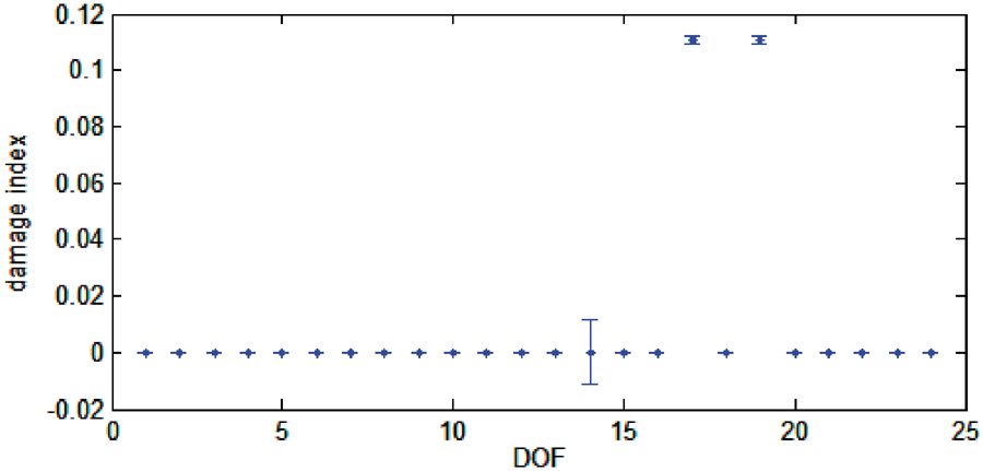
From the computed results it can be seen that for the two-stage damage identification method the measurement noise hardly affects the damage identification results.

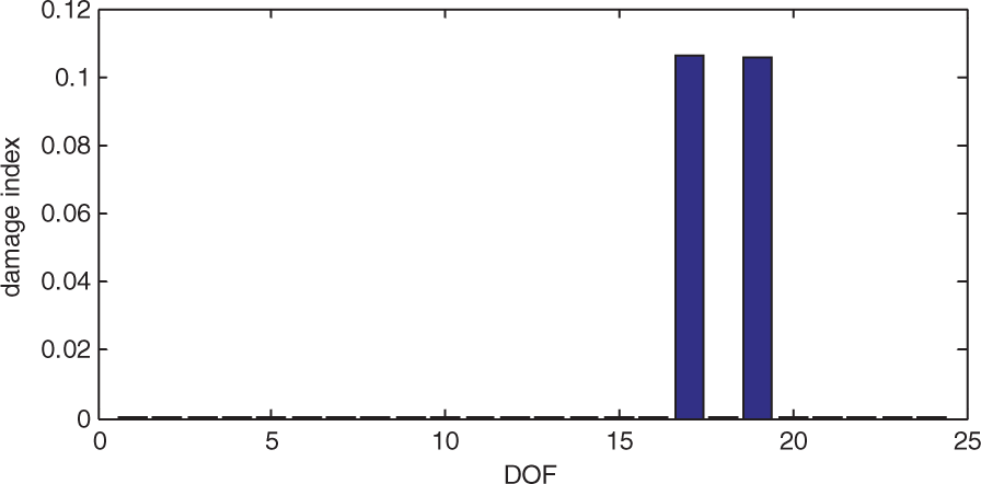
In general, the effects of the errors in mass and stiffness matrices should also be considered. The directness generalized inverse method with noise cannot identify the true damage locations and extent. Therefore, we just study the proposed two stage method. Here, the error in stiffness matrix is 4% and the error in mass matrix is 2%. If the measurement noise of frequency responses is not considered, the computed results of damage localization are shown in Figure 6, where it can be observed that the changes of damage index also occur in d.f. 17 and 19. So, element 10 should be the suspected damage element. Here, we select d.f. 17 as the reduced d.f‥ Then, we use equations (14) and (15) to calculate damage extent. The computed damage coefficient is shown as follows:

Figure 6.

Damage index of the two-stage method with errors in stiffness and mass matrices when damage occurs in the 10th element.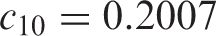

From the computed results it can be seen that the small errors in mass and stiffness matrices have a small effect on the damage identification results.

For the two-stage damage identification method, the measurement noise of responses and the errors of massand stiffness matrices should be considered, simultaneously. Here, the errors in stiffness and mass matrices are 4% and 2%, respectively. The noise level is 0.02. The computed results of damage localization are shown in Figure 7, where it can be observed that the effect of measurement errors mainly occurs in d.f. 14, and it also has an effect on d.f. 17 and 19. Thus, we can deem that the changes of damage index mainly occur in d.f. 14, 17 and 19. However, we cannot find the matching d.f. change around d.f. 14. We cannot infer other suspected damage elements from the change of d.f. 14. So, element 10 should be the suspected damage elements. Here, we select d.f. 17 as the reduced d.f‥ Then, we use equations (15) and (22) to calculate damage coefficient and the noise standard variance, respectively. The computed results of the damage coefficient and standard variance are

Figure 7.

Damage index of the two-stage method with noise and errors when damage occurs in the 10th element (error of stiffness matrix 4%, error of mass matrix 2%, noise level 0.02, damage index of the perturbations along with ±1σ error bars).

From the computed results it can be seen that for single damage problem the effect of both the measurement noise and the errors is small.

5.2. Case 2

In case 2, damage occurs in elements 9 and 21 with 20% and 25% stiffness reduction, respectively. The results of numerical calculations of the directness generalized inverse method are shown in Figure 8, where it can be seen that elements 9 and 21 are the suspected damage elements. The damage extent values of elements 9 and 21 are 0.1833 and 0.0890. Thus, the localization results of the directness generalized inverse method are good but the quantification results are weak.

Figure 8.

Identification result of directness generalized inverse method when damages occur in 9th and 21st elements.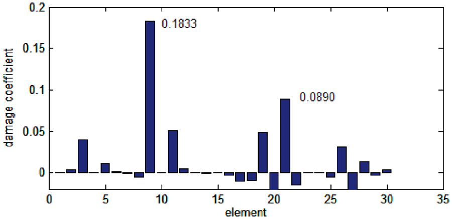

The measurement noise was considered for the directness generalized inverse method. When the noise level is 0.02, the computed results of the directness generalized inverse method with noise are shown in Figure 9, which shows the standard deviations of the damage coefficients. From Figure 9 it can be observed that the effects of the measurement noise far exceed the true damage. Thus, when the noise level is 0.02, the directness generalized inverse method cannot identify the true damage locations and extent.

Figure 9.

Identification result of directness generalized inverse method with noise when damage occurs in 9th and 21st elements (noise level 0.02, damage coefficients of the perturbations along with ±1σ error bars).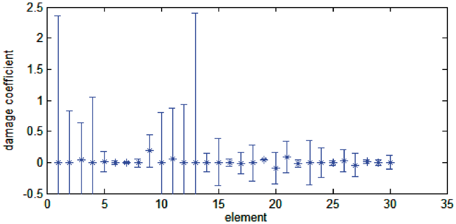

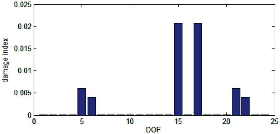
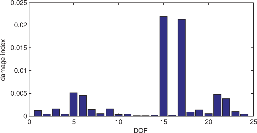
The proposed two-stage damage identification method was also used in this case. First, it is necessary to analyze damage location by using damage index. The computed results of damage localization are shown in Figure 10, where it can be observed that the changes of damage index occur in d.f. 5, 6, 15, 17, 21 and 22. And from Figure 1 it can be seen that the element which correlates with d.f. 5, 6, 21 and 22 is element 21, and the element which correlates with d.f. 15 and 17 is element 9. So, elements 9 and 21 should be the suspected damage elements. Thus, the number of suspected damage elements ND = 2. Here, we select d.f. 17 and 22 as reduced d.f. to calculate damage extent. Then, from equation (15) we can obtain the damage coefficients. The computed damage coefficients are listed as follows:

Figure 10.

Damage index of the two-stage method when damages occur in the 9th and 21st elements.

The identification results are equal to the true damage extent.

The effect of measurement noise should also be considered for the two-stage damage identification method. When the noise level is 0.02, the computed results of damage localization are shown in Figure 11. From Figure 11 it can be observed that the maximum effect of measurement errors still occurs in d.f. 14. Maybe the reason is the large displacement caused by the exciting force in the excitation location. Consider both the change of damage index and the effect of measurement noise; we can deem that the changes of damage index occur in d.f. 5, 6, 14, 15, 17, 21 and 22. And from Figure 1 it can be seen that the element which correlates with d.f. 5, 6, 21 and 22 is element 21; the element which correlates with d.f. 15 and 17 is element 9; and the element which correlates with d.f. 14 and 15 is element 8. The three elements caused the changes of damage index of d.f. 5, 6, 14, 15, 17, 21 and 22. So, elements 8, 9 and 21 should be the suspected damage elements. Thus, the number of suspected damage elements ND = 3. Here, we select d.f. 15, 17 and 22 as reduced d.f. to calculate damage extent. Then from equation (15) we can obtain the damage extent. The computed results of the damage coefficients and standard variances are

Figure 11.

Damage index of the two-stage method with noise when damages occur in the 9th and 21st elements (noise level 0.02, damage index of the perturbations along with ±1σ error bars).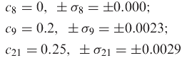

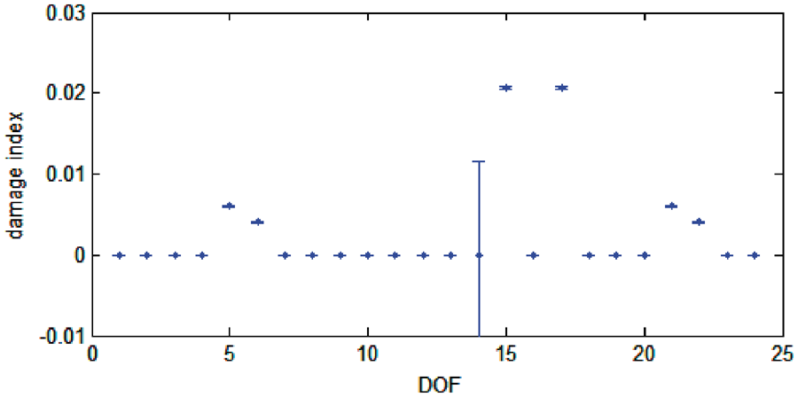
Therefore, we can tell that element 8 is not the true damage element. And it can be seen that for the two-stage damage identification method the effect of measurement noise is very small.

In general, the effects of the errors in mass and stiffness matrices should also be considered. Here, the errors in stiffness and mass matrices are 4% and 2%, respectively. If the measurement noise of responses is not considered, the computed results of damage localization are shown in Figure 12, where it can be observed that the big changes of damage index occur in d.f. 5, 6, 15, 17, 21 and 22 if the small changes are ignored. So, elements 9 and 21 should be the suspected damage elements. Thus, the number of suspected damage elements ND = 2. Here, we select d.f. 17 and 22 as reduced d.f. to calculate damage extent. Then, from equation (15) we can obtain the damage coefficients. The computed damage coefficients are listed as follows:

Figure 12.

Damage index of the two-stage method with errors in stiffness and mass matrices when damages occur in the 9th and 21st elements.

From the computed results it can be seen that the errors in mass and stiffness matrices have a small effect on the damage identification results.

For the two-stage damage identification method, the measurement noise of responses and the errors of mass and stiffness matrices should be considered, simultaneously. Here, the errors in stiffness and mass matrices are 4% and 2%, respectively. The noise level is 0.02. The computed results of damage localization are shown in Figure 13, where it can be observed that the maximum effect of measurement errors still occurs in d.f. 14. This could be because of the large displacement caused by the exciting force in the excitation location. Consider both the change of damage index and the effect of measurement noise; we can deem that the big changes of damage index occur in d.f. 5, 6, 14, 15, 17, 21 and 22 if the small changes are ignored. Similarly, elements 8, 9 and 21 should be the suspected damage elements. Thus, the number of suspected damage elements ND = 3. Here, we select d.f. 15, 17 and 22 as reduced d.f. to calculate damage extent. Then from equation (15) we can obtain the damage extent. The computed results of the damage coefficients and standard variances are

Figure 13.

Damage index of the two-stage method with noise and errors when damage occurs in the 9th and 21st elements (error of stiffness matrix 4%, error of mass matrix 2%, noise level0.02, damage index of the perturbations along with ±1σ error bars).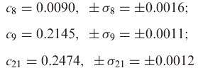

It can be seen that for the two-stage damage identification method the effect of both the measurement noise and the errors is small.

From the two cases, we can observe that it is difficult for the directness generalized inverse method to successfully identify structural damage. In case 1, the directness generalized inverse method can identify the single damage if the noise isn’t considered. When the measurement noise is taken into account, the directness generalized inverse method cannot successfully identify the single damage. In case 2, the directness generalized inverse method can approximately identify the multiple damage locations but cannot identify the damage extent. If the measurement noise is considered; the directness generalized inverse method cannot successfully identify the damage locations and extent. Here, the proposed two-stage damage identification method shows the potential to detect damage. The identification results of the two-stage method are very good whether the measurement noise is considered or not. And from the two cases, it can be seen that along with the increase of the suspected damage elements, the accuracy of identification results of the two-stage method will decrease.

6. Conclusions

A two-stage damage identification method using frequency responses and statistical theory to detect structural damage has been presented. The damage sites are first identified by using the damage index, and then the d.f. reduction method is applied to detect the damage extent. The numerical examples demonstrate that this two-stage method is effective and attractive for the practical use. When the measurement noise is considered, the two-stage method can estimate the damage location and extent with good accuracy. And the identification results of the two-stage method are better than those of the directness generalized inverse method. The proposed method would be applicable to a lightly damped structure where stiffness changes would not affect significantly the damping property of the structure. In general, if there are too many damaged elements in a structure, it is difficult for the two-stage method to identify structural damage locations. The damping change of structural damage is also neglected for the proposed method. Therefore, we think that the damping and multi-damage problem should be considered in future research.

Footnotes

Funding

This work was supported by the Fundamental Research Funds for the Central Universities (Project No. CDJZR10200007).

References

Dong

Fan

Chen

(2002) Theory and method for structural intelligent health diagnosis. China Rail Way Science 23: 11–24.

Guo

Zhang

(2006) A weighted balance evidence theory for structural multiple damage localization. Computer Methods in Applied Mechanics and Engineering 195(44–47): 6225–6238.

Hearn

Testa

(1991) Modal analysis for damage detection in structures. ASCE Journal of Structure Engineering 117(10): 3042–3063.

Law

Shi

Zhang

(1998) Structural damage detection from incomplete and noisy modal data. ASCE Journal of Engineering Mechanics 124(11): 1280–1288.

Maia

NMM

Silva

JMM

Almas

EAM

(2003) Damage detection in structures from mode shape to frequency response function methods. Mechanical System and Signal Processing 17(3): 489–498.

Park

Cudney

Inman

(2000) An integrated health monitoring technique using structural impedance sensors. Journal of Intelligent Material Systems and Structures 11(6): 448–455.

Park

(2003) Damage detection using spatially incomplete frequency response functions. Mechanical Systems and Signal Processing 17(3): 519–532.

Norman

(1976) Matrix Theory and its Applications New York: Marcel Dekker.

Ren

Roeck

(2002) Structural damage identification using modal data I: simulation verification. Journal of Structural Engineering 128(1): 87–95.

10.

Salawu

(1997) Detection of structural damage through changes in frequency: a review. Engineering Structures 19(9): 718–723.

11.

Schulz

Naser

(1998) Locating structural damage using frequency response functions. Journal of Intelligent Material Systems and Structures 9(11): 899–905.

12.

Shi

Law

Zhang

(2000a) Optimum sensors placement for structural damage detection. ASCE Journal of Engineering Mechanics 126(11): 1173–1179.

13.

Shi

Law

Zhang

(2000b) Damage localization by directly using incomplete mode shapes. ASCE Journal of Engineering Mechanics 126(6): 656–660.

14.

Zheng

Liu

Chen

(2001) Structural damage assessment based on frequency response function. Mechanical Science and Technology 20(3): 479–480 [in Chinese].

15.

Zimmerman

Simmermacher

Kaouk

Structural damage detection using frequency response function, (1995) Proceedings of the 13th International Modal Analysis Conference, 13–16 February 1995, Nashville, Tennessee, USA, 179–184.