Semi-active vibration suppression of a space truss structure using a fault tolerant controller

Abstract

In recent years, magneto-rheological (MR) dampers have been used to control the response of structures. This paper presents the design and application of an H_∞ fault detection and isolation (FDI) filter and fault tolerant controller (FTC) for truss vibration control systems using MR dampers. A linear matrix inequality formulation is used to design a full order robust H∞ filter to estimate faulty input signals. A fault tolerant H_∞ controller is designed for the combined system of plant and filter, minimizing the control objective selected in the presence of disturbances and faults. A truss structure with an MR damper is used to validate the FDI and FTC controller design through numerical simulations. The residuals obtained from the filter through simulation clearly identify the fault signals. The simulation results of the proposed FTC controller confirm its effectiveness for vibration suppression of the faulty truss system.

Keywords

Fault tolerant control magneto-rheological (MR) dampers semi-active vibration control truss structure

1. Introduction

Space truss structures are always subjected to a variety of dynamic perturbations produced by the crew, transient thermal states during orbit and micrometeorites, among others (Song et al., 2002). Truss-type space structures can carry important, sensitive pieces of equipment, such as interferometers, antennae and other vibration-sensitive instrumentation, whose readings can be disturbed by the vibrations caused by the aforementioned dynamic perturbations. However, because of launch constraints, these truss structures must be lightweight and, consequently, they are prone to vibrations. Various active vibration suppression strategies have been proposed in the past to suppress vibration of the spacecraft truss structures. Active control systems operate by using external energy supplied by actuators to impart forces on the structure, generally depending on a sizeable power supply for operation. However, in the case of space trusses, there are still a number of questions that must be addressed, including stability, cost effectiveness, reliability, and power requirements. For instance, active systems have the ability to input mechanical energy into the structural system, making them capable of generating instabilities due to un-modeled dynamics and nonlinearities or even equipment failure (e.g., power source, sensors, control hardware/software, etc.). Additionally, the need for sizeable power supplies and large control forces may make them costly to install and maintain (Dyke and Spencer, 1997). Semi-active systems offer another alternative in truss control. A semi-active control device is defined as one that cannot increase the mechanical energy in the controlled system but has properties that can be dynamically varied. Semi-active systems are an attractive option because they possess the adaptability of active control systems, yet are intrinsically stable and operate using very low power. Additionally, semi-active control devices do not require large power sources such as those associated with active control systems (Li et al., 2005; Liu et al., 2007), making them quite attractive for seismic applications. One semi-active device that appears to be particularly promising for truss applications is the magneto-rheological (MR) damper.

To simplify the control of the truss structures, the development of an adaptive-passive system is proposed, one which initially tunes the parameters of the system and then achieves vibration suppression through MR fluid based damping devices. MR dampers have been developed as semi-active vibration devices in recent years (Dyke et al., 1996; Li et al., 2010; Oh and Onoda, 2002; Spencer et al., 1997, 1998). MR fluid, a material which responds to applied magnetic fields, is used as the operating fluid. MR fluids alter their viscosity according to the applied magnetic field and exhibit nonlinear properties like a typical Bingham fluid. In MR dampers, electromagnets are used to generate the required magnetic field. The force generated in the MR damper is therefore controlled by adjusting the electric current supplied to the electromagnets (Sodeyama and Sunakoda, 2003). The advantage of this adaptive-passive system lies in its fail-safe design. Unlike active control, which requires active energy for vibration suppression, this MR fluid design would utilize its passive properties in the event of energy loss.

Fault tolerant schemes in engineering systems provide early warnings of faulty sensors, actuators, or system components. In this paper, a component fault refers to a change in the operating behavior of a component such that the new behavior differs significantly from what is defined as normal behavior for that component. Common examples of such faults include bias errors in the output of a sensing device and loss of function for an actuating device (Chen and Patton, 1999). Health monitoring systems are needed to provide early notification of faults before they lead to catastrophic failure so that remedial actions can be carried out to retain the system stability and performance. Consequently, the fault detection and isolation (FDI) and fault tolerant control (FTC) problems have received considerable attention in control systems literature (Chen and Nagarajaiah, 2007, 2008; Diallo et al., 2004; Koh et al., 2005a,b; Li et al., 2007; Maki et al., 2001; Narasimhan et al., 2008).

Most applications of fault tolerant control schemes are based or partially based on hardware redundancy. The use of this kind of hardware redundancy is common, but it carries with it the problem of additional equipment, maintenance cost, and space requirements. In some engineering environments, extra space for redundant sensors and actuators are hard to come by.

Recently developed analytical redundancy techniques use residue signals to monitor the health of systems. The term residue is defined as a signal that is zero when the system functions properly and non-zero when some abnormal behavior is observed. This residual signal indicates faulty information in the system and can be used not only for fault detection, but also for fault identification. Further more, it also provides basic information for the fault tolerant control purpose of use. It is a natural way to cope with the FTC Problem by employing fault diagnosis information online.

There are several approaches to generate the residual signals and to build the FTC scheme, such as the unknown input observer, the H_∞ method, the Kalman filter, and the H2/LQG techniques. (Hamouli et al., 2004; Douglas and Speyer, 1999; Eryurek and Upadhyaya, 1995). Among these approaches, the H_∞ optimization based methods have attracted much attention due to their explicit address of robustness issues. In this work, an H_∞ FDI filter is developed based on the system identification model of the truss. The main design goal of this FDI filter is to detect and identify sensor failure of the truss structure system. The linear matrix inequality (LMI) formulation of the FDI H_∞ filter is obtained based on the famous bounded real lemma. An FTC H_∞ control scheme is proposed and it successfully retains the vibration suppression level when the sensors on the truss have partially failed.

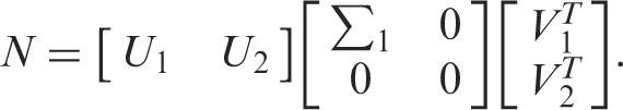
The notation to be used is given as follows: Given a real matrix N, the orthogonal complement $N^{⊥}$ is defined as the (possibly non-unique) matrix with maximum row rank that satisfies $N^{⊥} N = 0$ and $N^{⊥} N^{⊥} >0$ . Hence, $N^{⊥}$ can be computed from the singular value decomposition of N as follows: $N^{⊥} = {TU}_{2}^{T}$ where T is an arbitrary nonsingular matrix and U₂ is defined from the singular value decomposition on N:

N = [\begin{matrix} U_{1} U_{2} \end{matrix}] [\begin{matrix} \sum_{1} 0 00 \end{matrix}] [\begin{matrix} V_{1}^{T} V_{2}^{T} \end{matrix}] .

The standard notation > (<) is used to denote the positive (negative) definite ordering of symmetric matrices. The i^th eigenvalue of a real symmetric matrix N will be denoted by λ_i(N) where the ordering of the eigenvalues is defined as $λ_{max} (N) = λ_{1} (N) \geq λ_{2} (N) \geq \dots \geq λ_{n} (N)$ . The maximum singular value of a (not necessarily square) matrix N will be denoted by $σ_{max} (N)$ , which is also its spectral norm $‖ N ‖$ . N⁺ will denote the Moore-Penrose generalized inverse of a matrix N.

2. H∞ fault detection filtering and H∞ fault tolerant control problems

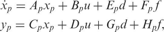
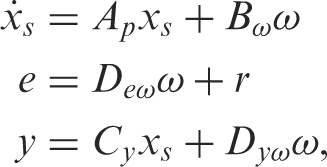
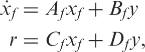
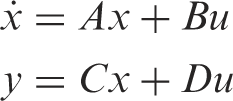
Consider the following state-space realization for a plant P given by

\begin{matrix} {\overset{\cdot}{x}}_{p} = A_{p} x_{p} + B_{p} u + E_{p} d + F_{p} f \\ y_{p} = C_{p} x_{p} + D_{p} u + G_{p} d + H_{p} f, \end{matrix}

(1)

where x_p is the state vector, u is the control input, d is the disturbance input, f is the fault input, y_p is the system output, and A_p, Bp, E_p, F_p, C_p, D_p, G_p and H_p are real matrices of appropriate dimensions. Suppose F is the unknown filter to be determined and has the following state-space representation

\begin{matrix} {\overset{\cdot}{x}}_{f} = A_{f} x_{f} + B_{f} u + E_{f} y \\ r = C_{f} x_{f} + D_{f} u + H_{f} f, \end{matrix}

(2)

where x_f is the filter state vector, u is the control input, r is the output vector and A_f, B_f, E_f, C_f, D_f, and H_f are real matrices of appropriate dimensions. Define the generalized disturbance, ω^T= [u, d, f]^T, and estimation error, e = r − f, as shown in Figure 1 (Bai, 2006). The H_∞ optimal filter problem is to find a dynamic filter to minimize the worst case estimation error energy over the energy of bounded generalized disturbance, that is,

{min}_{F} {sup}_{ω \in L_{2}} \frac{‖ e ‖_{2}}{‖ ω ‖_{2}} .

(3)

Figure 1.

Block diagram of the H_∞ fault detection filter.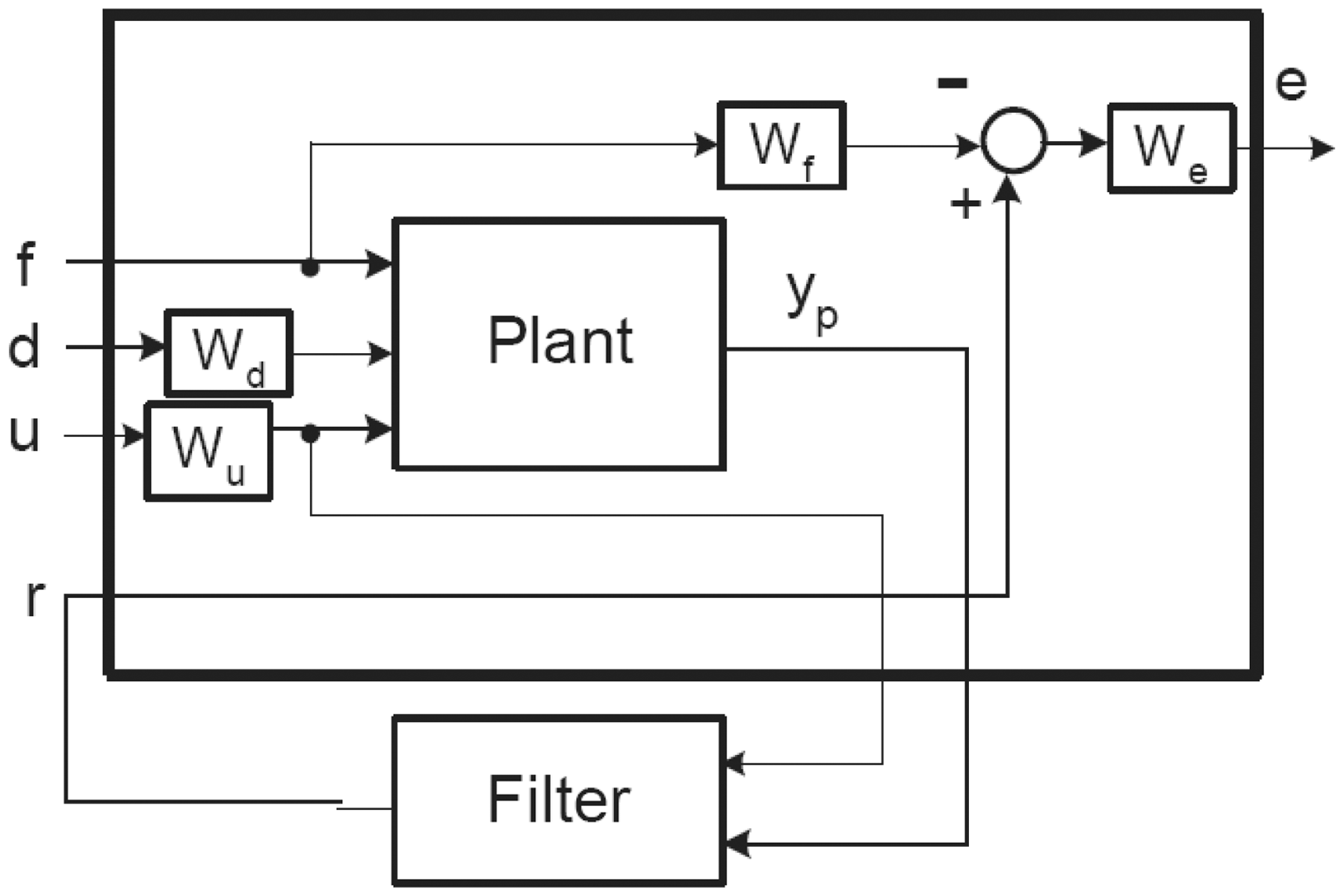

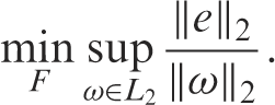
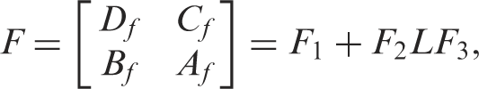
The expression (3) is equivalent to minimizing the H_∞ norm of the transfer function $T_{ω e}$ between the generalized disturbance input and the error of the fault estimation (Wang and Song, 2011). Similarly, the γ-sub-optimal H_∞ FDI filtering problem is to find, if there exists, a filter, F, such that $‖ T_{ω e} ‖ <γ$ , where γ is a given positive scalar. (Grigoriadis and Skelton, 1996, 1998)

Using the linear fractional transformation (LFT), the space state realization of the transfer function (or transfer matrix) $T_{ω e}$ (see the bold black square in Figure 1) can be obtained as

\begin{matrix} {\overset{\cdot}{x}}_{s} = A_{p} x_{s} + B_{ω} ω \\ e = D_{e ω} ω + r \\ y = C_{y} x_{s} + D_{y ω} ω, \end{matrix}

(4)

where

x_{s} = x_{p}

B_{ω} = [B_{p}, E_{p}, F_{p}]

D_{e ω} = [0, 0, - I]

C_{y} = [0, C_{p}]^{T}

and

D_{y ω} = [\begin{matrix} I 00 D_{p} G_{p} H_{p} \end{matrix}]

(i.e.

y^{T} = [u, y_{p}]^{T}

). Thus, the optimal or γ-sub-optimal H_∞ FDI filtering problem can be formulated as the standard H_∞ control problem and then solved by the Raccati or LMI approach. (Mahmoud et al., 2003; Skelton et al., 1998)

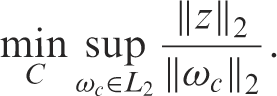
It is well known that the solution to the H_∞ control problem is a powerful tool in solving the disturbance attenuation problem. The H_∞ optimal fault tolerant control design problem is to find a dynamic controller, C, to minimize the worst case performance output energy over the energy of bounded generalized disturbance, $ω_{c}^{T} = [f, d]^{T}$ . That is,

{min}_{C} {sup}_{ω_{c} \in L_{2}} \frac{‖ z ‖_{2}}{‖ ω_{c} ‖_{2}} .

(5)

The control strategy of the H_∞ control FTC controller is shown in Figure 2.

Figure 2.

Block diagram of the proposed fault tolerant controller.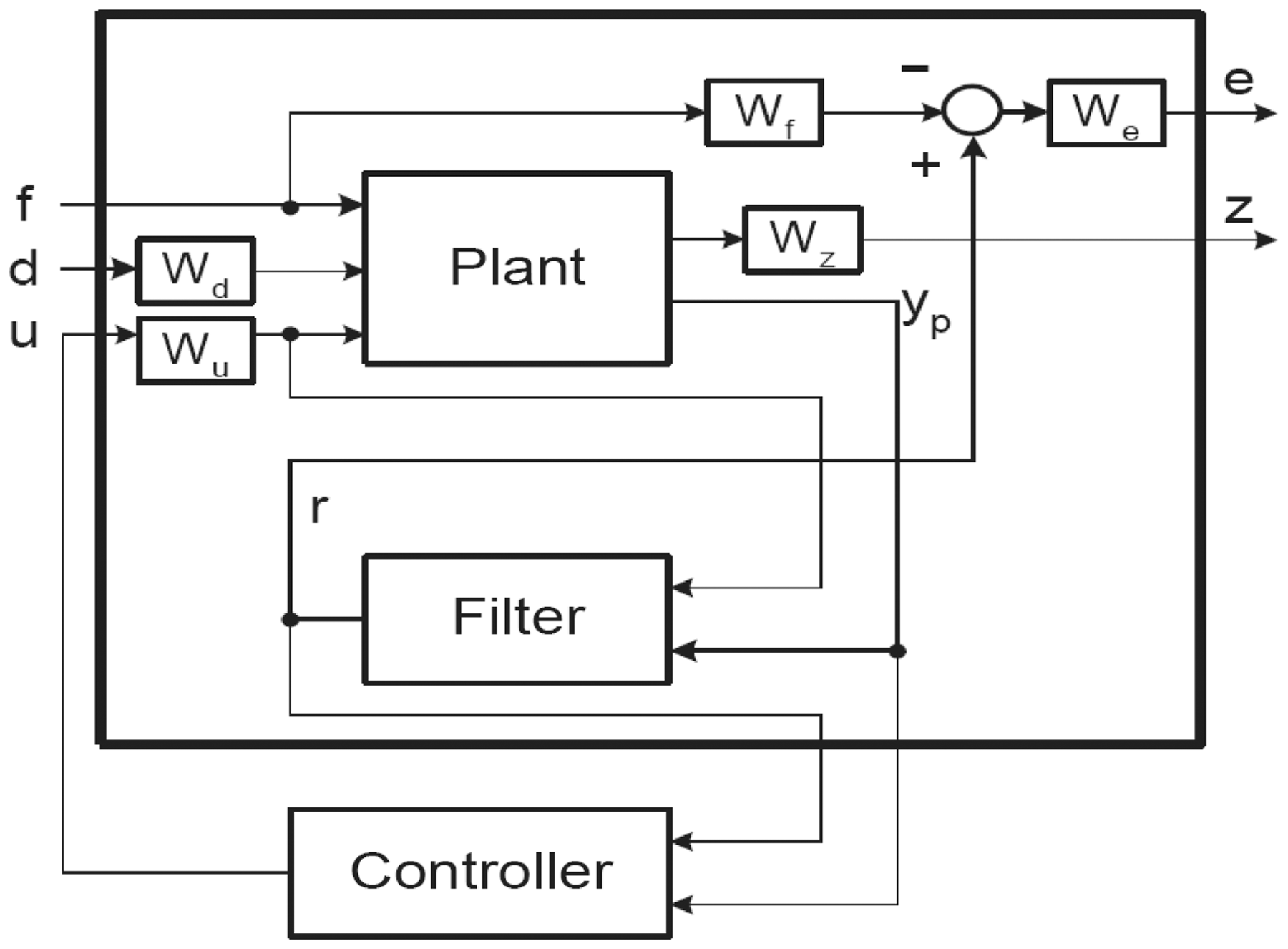

3. H∞ filter design using linear matrix inequality

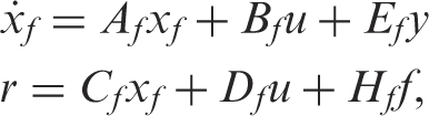
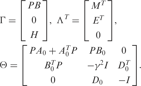
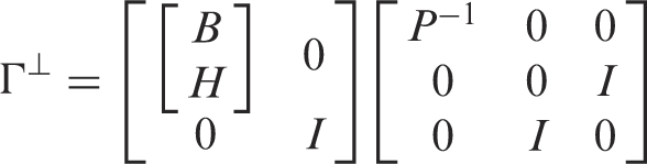
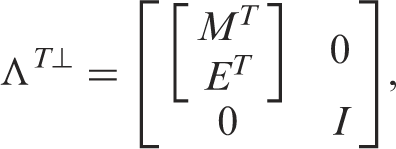
Consider a system with order n_p that has the state space representation of (4). The following theorem is useful in designing a state filter F of order n_f_, which is less than or equal to n_p_, with the following state space representation,

\begin{matrix} {\overset{\cdot}{x}}_{f} = A_{f} x_{f} + B_{f} y \\ r = C_{f} x_{f} + D_{f} y, \end{matrix}

(6)

where x_f is the state vector, r is the filter output that estimates the fault, y is the output of the generalized plant shown in equation (6), and A_f. B_f, C_f and D_f are real matrices of appropriate dimensions. The filter can be written in compact notation as

F = [\begin{matrix} D_{f} C_{f} B_{f} A_{f} \end{matrix}] .

(7)

There exists an $n_{f}^{th}$ order H_∞ filter F to solve the γ-sub-optimal H_∞ FDI filtering problem if and only if there exists matrices X and Y such that the following conditions are satisfied (Gahinet and Apkarian, 1994; Grigoriadis, 1995):

[\begin{matrix} {XA}_{s} + A_{s}^{T} X {XB}_{ω} B_{ω}^{T} X - γ^{2} I \end{matrix}] <0

(8)

{[\begin{matrix} C_{y}^{T} D_{y ω}^{T} \end{matrix}]}^{⊥} [\begin{matrix} {YA}_{s} + A_{s}^{T} Y {YB}_{ω} B_{ω}^{T} Y D_{e ω}^{T} D_{e ω} - γ^{2} I \end{matrix}] [\begin{matrix} C_{y}^{T} D_{y ω}^{T} \end{matrix}] <0

(9)

[\begin{matrix} X I I Y \end{matrix}] \geq 0

(10)

rank (Y - X) \leq n_{f} .

(11)

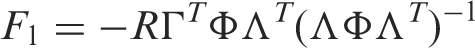
In this case, all such filters are given by

F = [\begin{matrix} D_{f} C_{f} B_{f} A_{f} \end{matrix}] = F_{1} + F_{2} {LF}_{3},

(12)

where

L \in R^{(n_{p} + n_{f}) \times (n_{p} + n_{f})}

is any matrix such that

‖ L ‖ <1

and R is any positive definite matrix such that

Φ = (Γ R Γ^{T} - Θ)^{- 1} >0

(13)

and

F_{1} = - R Γ^{T} Φ Λ^{T} (Λ Φ Λ^{T})^{- 1}

(14)

F_{2} = (R - R Γ^{T} [Φ - Φ Λ^{T} (Λ Φ Λ^{T})^{- 1} Λ Φ] Γ R)^{1 / 2}

(15)

F_{3} = (Λ Φ Λ^{T})^{- 1 / 2} .

(16)

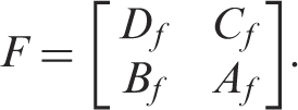
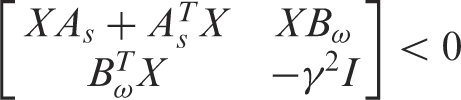
To prove the above theorem, we need the following bounded real lemma and projection lemma (Iwasaki and Skelton, 1994).

Consider a stable linear time invariant system

\begin{matrix} \overset{\cdot}{x} = Ax + Bu \\ y = Cx + Du \end{matrix}

(17)

with transfer function

T (s) = C (sI - A)^{- 1} B + D

. Let γ be a given positive scalar. Then,

‖ T ‖_{\infty} <γ

if and only if there exists a matrix P > 0 satisfies the following LMI (Geromel et al., 1996):

[\begin{matrix} A^{T} P + PA PB C^{T} B^{T} P - γ^{2} I D^{T} C D - I \end{matrix}] <0 .

(18)

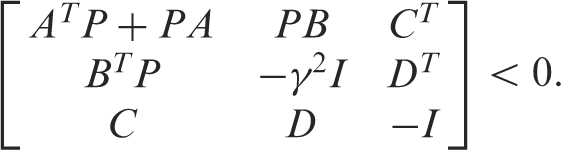
Consider a symmetric matrix $Θ \in R^{m \times m}$ and two matrices Γ and Λ with column dimension m. Let $Γ^{⊥}$ and $Λ^{⊥}$ denote the orthogonal complement of Γ and Λ respectively. With this notation, there exists a matrix Ω of compatible dimension such that (Boyd et al., 1994)

Θ + Γ Ω Λ + (Γ Ω Λ)^{T} <0

(19)

if and only if

Γ^{T} Θ Γ^{⊥ T} <0

(20)

and

Λ^{T ⊥} Θ Λ^{T ⊥ T} <0

(21)

are satisfied.

Proof of theorem 1

Define the state vector $x_{c} = {[\begin{matrix} x_{s} x_{f} \end{matrix}]}^{T}$ and write the closed-loop plant and filter system in the state space form as

\begin{matrix} {\overset{\cdot}{x}}_{c} = A_{c} x_{c} + B_{c} ω \\ e = C_{c} x_{c} + D_{c} ω, \end{matrix}

(22)

where

A_{c} = A_{0} + BFM

B_{c} = B_{0} + BFE

C_{c} = C_{0} +

HFM,

D_{c} = D_{0} + HFE

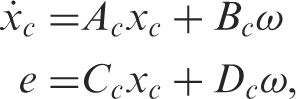
Substituting A_c, B_c, C_c and D_c into the bounded real lemma (18) and writing it in the form of inequality (19), we have

Noticing that

Γ^{⊥} = [\begin{matrix} [\begin{matrix} B H \end{matrix}] 0 0 I \end{matrix}] [\begin{matrix} P^{- 1} 00 00 I 0 I 0 \end{matrix}]

and

Λ^{T ⊥} = [\begin{matrix} [\begin{matrix} M^{T} E^{T} \end{matrix}] 0 0 I \end{matrix}],

by partitioning P and P⁻¹ as

P = [\begin{matrix} Y Y_{12} Y_{12}^{T} Y_{22} \end{matrix}], P^{- 1} = [\begin{matrix} Z Z_{12} Z_{12}^{T} Z_{22} \end{matrix}]

(23)

and setting

X = Z^{- 1},

(24)

the inequality (8) to (9) can be easily obtained after some simple algebraic manipulations.Using the inverse of block matrix formula, (21) to (22) can be written as

X = Y - Y_{12} Y_{22}^{- 1} Y_{12}^{T} .

Hence,

Y - X = Y_{12} Y_{22}^{- 1} Y_{12}^{T} \geq 0,

(25)

or, equivalently, using the Shur complement formula.

[\begin{matrix} X I I Y \end{matrix}] \geq 0 .

Moreover, we have

rank (Y - X) = rank (Y_{12} Y_{22}^{- 1} Y_{12}^{T}) \leq n_{f} .

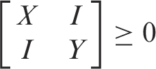
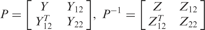
The free parameters can be used to optimize the system properties. A filter of order n_f < n_p exists if and only if X and Y satisfy the following rank constraint:

rank (X - Y) \leq n_{f} .

For the full order (n_f = n_p) H_∞ filter problem, a minimization of γ is possible because the non-convex rank condition (11) is automatically satisfied (Bai and Grigoriadis, 2005). Thus the LMI problem has only convex constraints on the matrix parameters X and Y for the full order filter design. However, the reduced order filter pair requires the inclusion of a non-convex rank constraint. Once this feasible pair is found, the Lyapunov matrix P is constructed as

P = [\begin{matrix} Y Y_{12} Y_{12}^{T} Y_{22} \end{matrix}],

where the partitioned blocks are computed from the decomposition (25). Consequently, the desired filter is obtained by solving (13) to (16).

4. Description of truss structures

The truss used in this research is located at Rice University and shown in Figure 3. This 8-bay, planar aluminum truss structure consists of 109 rod elements connected at 36 nodes. The total length of the truss is 4 m with each bay 0.5 m long and with rod elements having a Young's modulus of $E = 7.58 \times 10^{7} N / m^{2}$ . All the members are 0.1 in. thick hollow tubes with an outer diameter of 0.5 in.

Figure 3.

The 8-bay truss used for the study.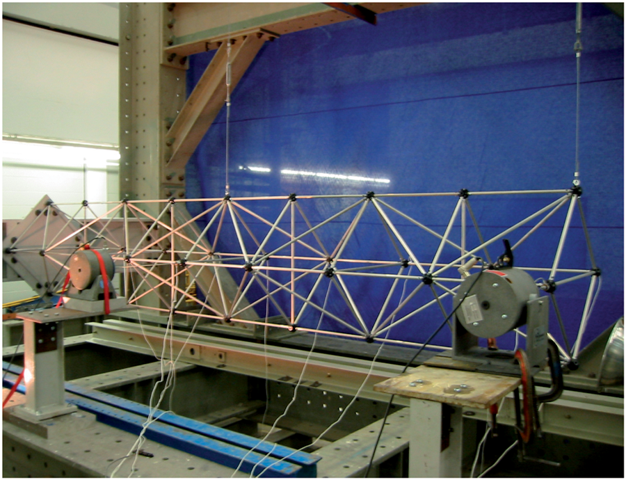

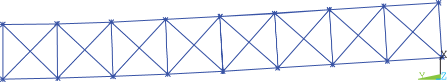
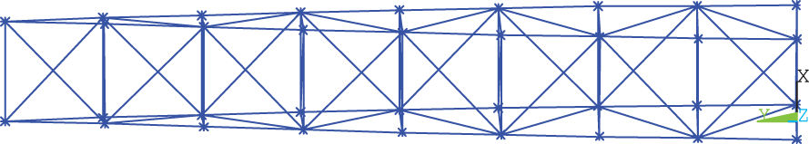
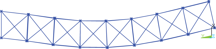
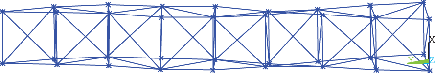
The truss can be simplified as a finite element model with 36 nodes and 109 members as shown in Figure 4. This truss has an electromechanical shaker mounted for excitation at node 4. Four accelerometers are mounted for monitoring of vibrations on the truss at node 1, 9, 13 and 17, respectively. An MR damper is installed between node 32 and 36 to reduce the vibration of the truss. The first four modes of the truss computed by finite element method (FEM) are shown from Figures 5 to 8.

Figure 4.

Finite element model of the truss.

Figure 5.

The first mode of the truss (13.68 Hz).

Figure 6.

The second mode of the truss (38.55 Hz).

Figure 7.

The third mode of the truss (66.46 Hz).

Figure 8.

The fourth mode of the truss (110.24 Hz).

Figure 9.

Comparison of output and identified model (from shaker to sensor 1).

Figure 10.

Comparison of output and identified model (from shaker to sensor 2).

Figure 11.

Comparison of output and identified model (from shaker to sensor 3).

Figure 12.

Comparison of output and identified model (from shaker to sensor 4).

Figure 13.

Bode diagram of identified model (from shaker to sensor 1).

Figure 14.

Bode diagram of identified model (from shaker to sensor 2).

Figure 15.

Bode diagram of identified model (from shaker to sensor 3).

Figure 16.

Bode diagram of identified model (from shaker to sensor 4).

Figure 17.

Comparison of output and identified model (from controller to sensor 1).

Figure 18.

Comparison of output and identified model (from controller to sensor 2).

Figure 19.

Comparison of output and identified model (from controller to sensor 3).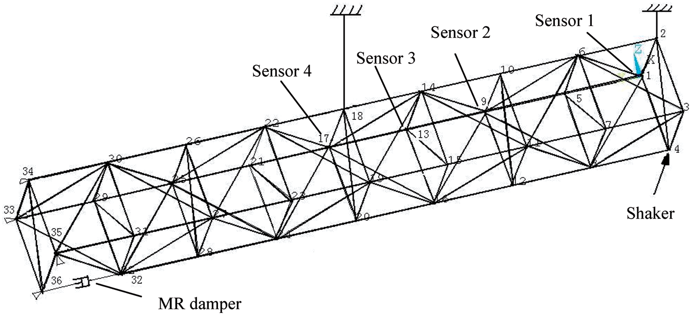

5. System identification

The approach of determining the transfer function using the mathematical modeling and finite element analysis is complex. The finite element models are sometimes not feasible for control purposes because their orders are too high to achieve the desired accuracy. However, the system identification technique based on input-output offers a rather simplistic approach to obtain the transfer function of the system. The input and the output signals from the system are analyzed in order to obtain a model.

In this work, the system identification algorithm used to identify the system is based on the Subspace method. A linear system can be represented in the state space innovations form as

\begin{matrix} x (t + 1) = Ax (t) + Bu (t) + Ke (t) \\ y (t) = Cx (t) + Du (t) + e (t), \end{matrix}

(26)

where e (t) is the innovations (i.e. the part of the output that cannot be predicted from the past data), x(t) is the state vector, y(t) is output, u(t) is the input and K is the Kalman gain.

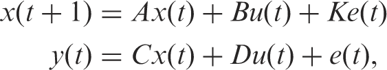
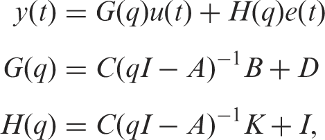
The subspace method can be used to estimate the A, B, C, D and K matrices. Assuming that x(t), y(t), and u(t) are known, the equation (26) becomes a linear regression. This will enable us to estimate the matrices C and D by the least square method and will lead us to determine e(t). Again, e(t) can be treated as a known signal and this will lead to the determination of A, B and K using the least squares method. The Kalman gain K is computed using the Riccati equation. In the above method, initially it is assumed that states x(t) are known, but they need to be determined. The states x(t) can be formed as linear combinations of the k-step-ahead predicted outputs. The predictor, in this method, can be determined using the k-step-ahead predictors by projections from the observed data sequences. The above model derived from the subspace method is then used as a base model for further refining the model by the prediction error method (PEM). In the time domain, the above system can be represented by using the shift operator q as

\begin{matrix} y (t) = G (q) u (t) + H (q) e (t) \\ G (q) = C (qI - A)^{- 1} B + D \\ H (q) = C (qI - A)^{- 1} K + I, \end{matrix}

(27)

where G(q) is the transfer function of the system, e(t) is the innovations, and I is the identity matrix. From the observed data of input, u, and output, y, the prediction errors can be computed as

e (t) = H^{- 1} (q) [y (t) - G (q) u (t)] .

(28)

The above error can now be parameterized by the state space matrices derived by the subspace method. The common parametric identification method is to determine estimates of G and H by minimizing

V_{N} (G, H) = \sum_{t = 1}^{N} e^{2} (t) .

(29)

This forms the basis for the PEM. The model is first initialized and further adjusted by optimizing the prediction error fit. Substantial details for system identification can be found in Ljung (1999) and MATLAB reference manual. MATLAB has a system identification toolbox to perform the above algorithm. The PEM first initializes the model by using the subspace algorithm and then minimizes the prediction error. In this paper, a state space realization that does not model the noise properties (i.e. an output error model), (K = 0), is considered. Thus, the implications will be on the predictors which will be based on the past inputs only.

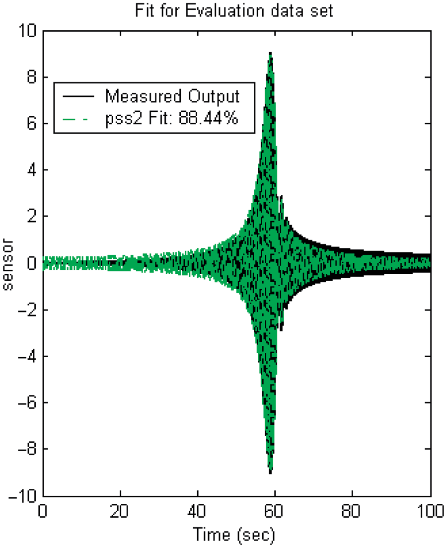
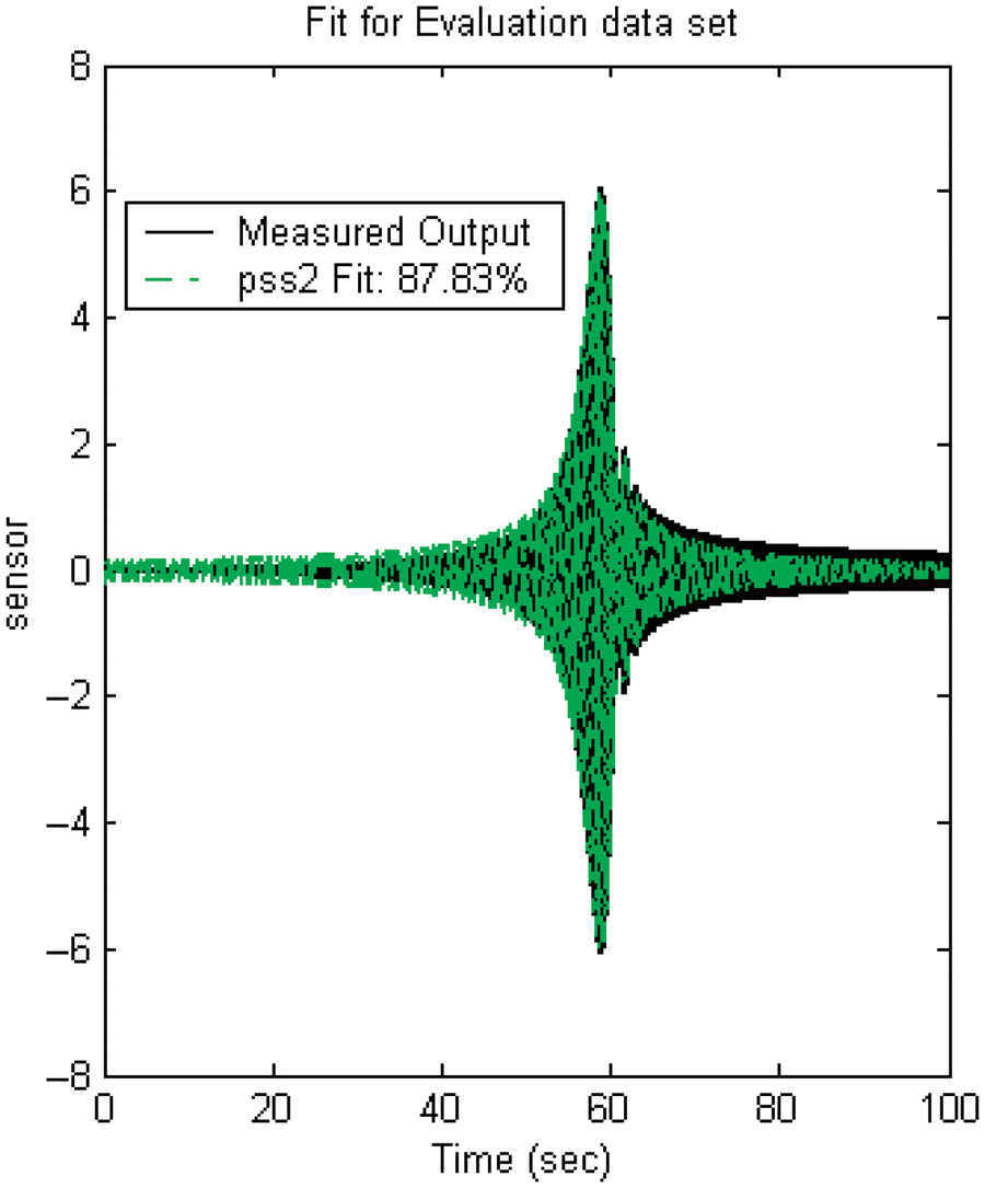
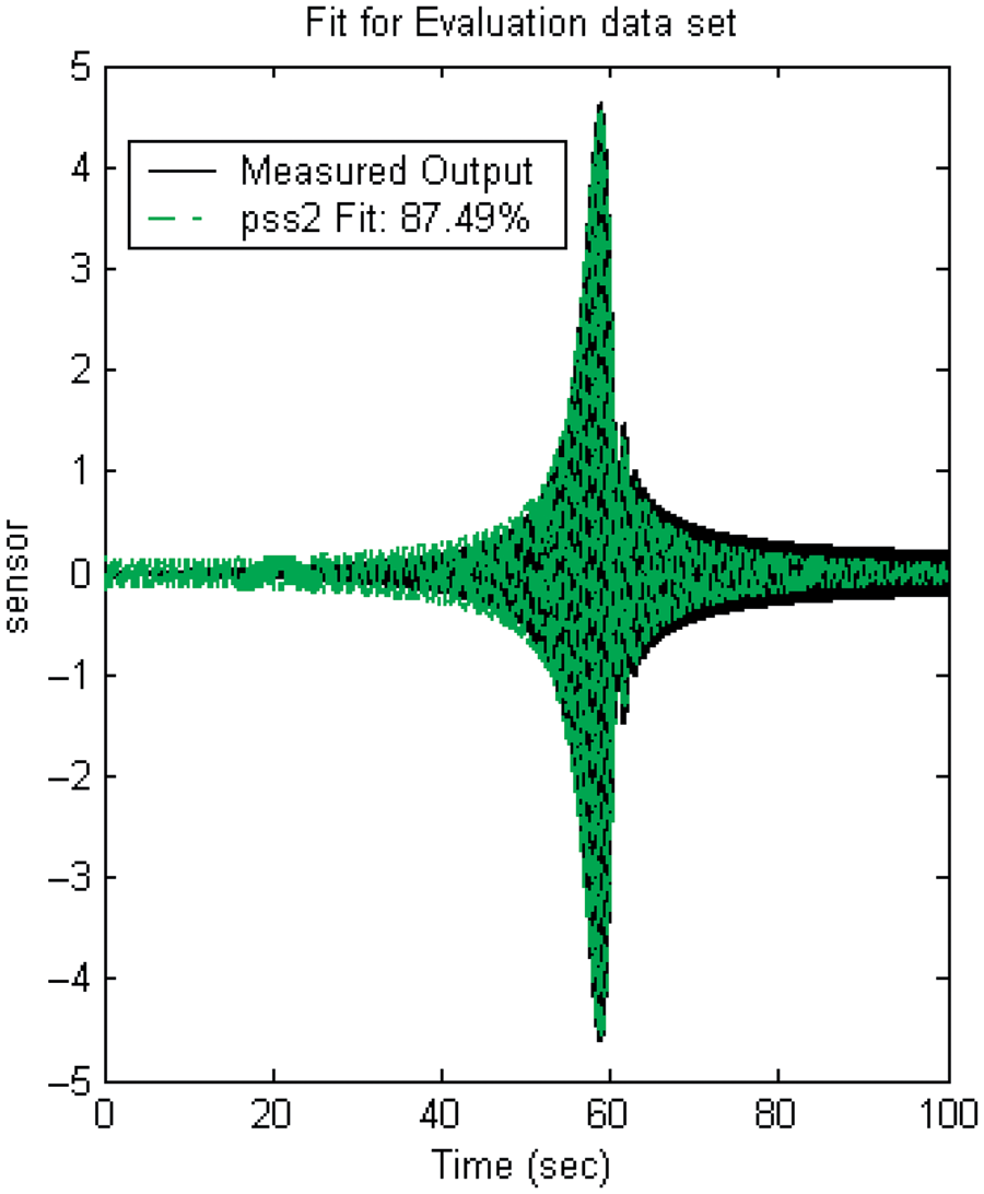
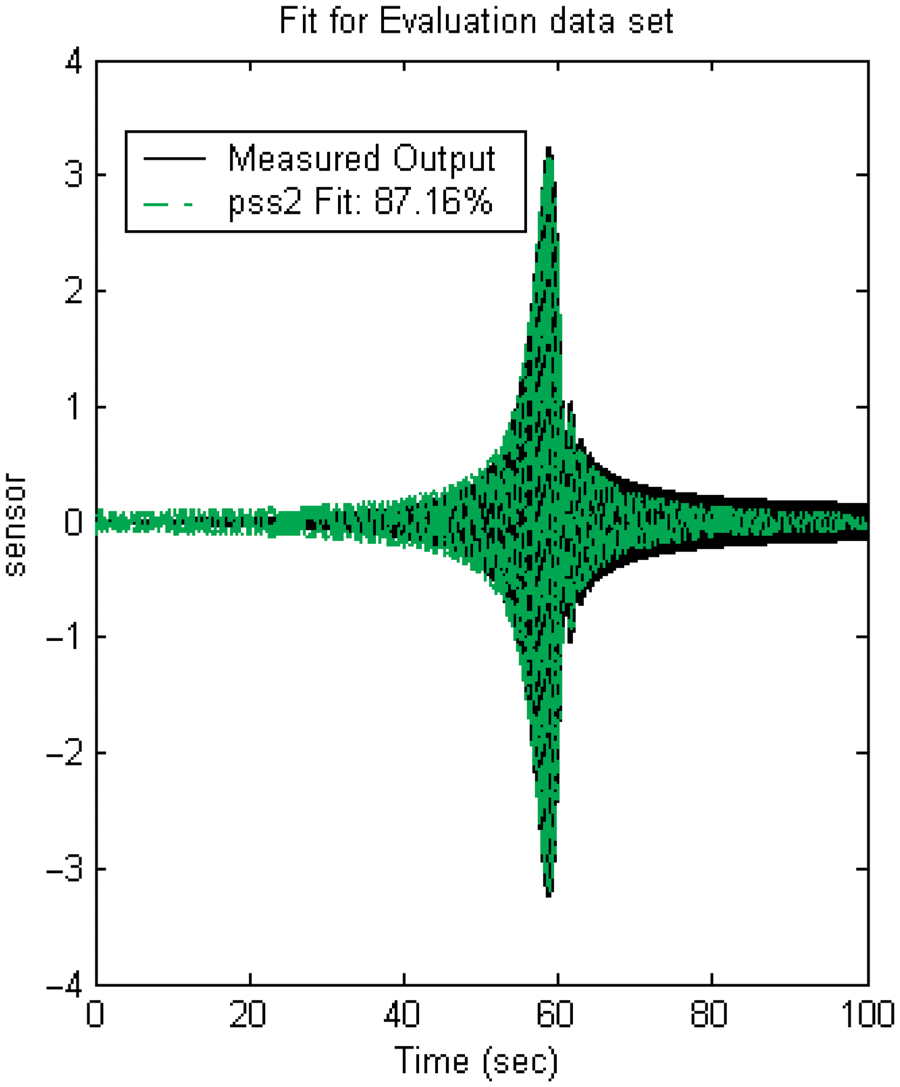
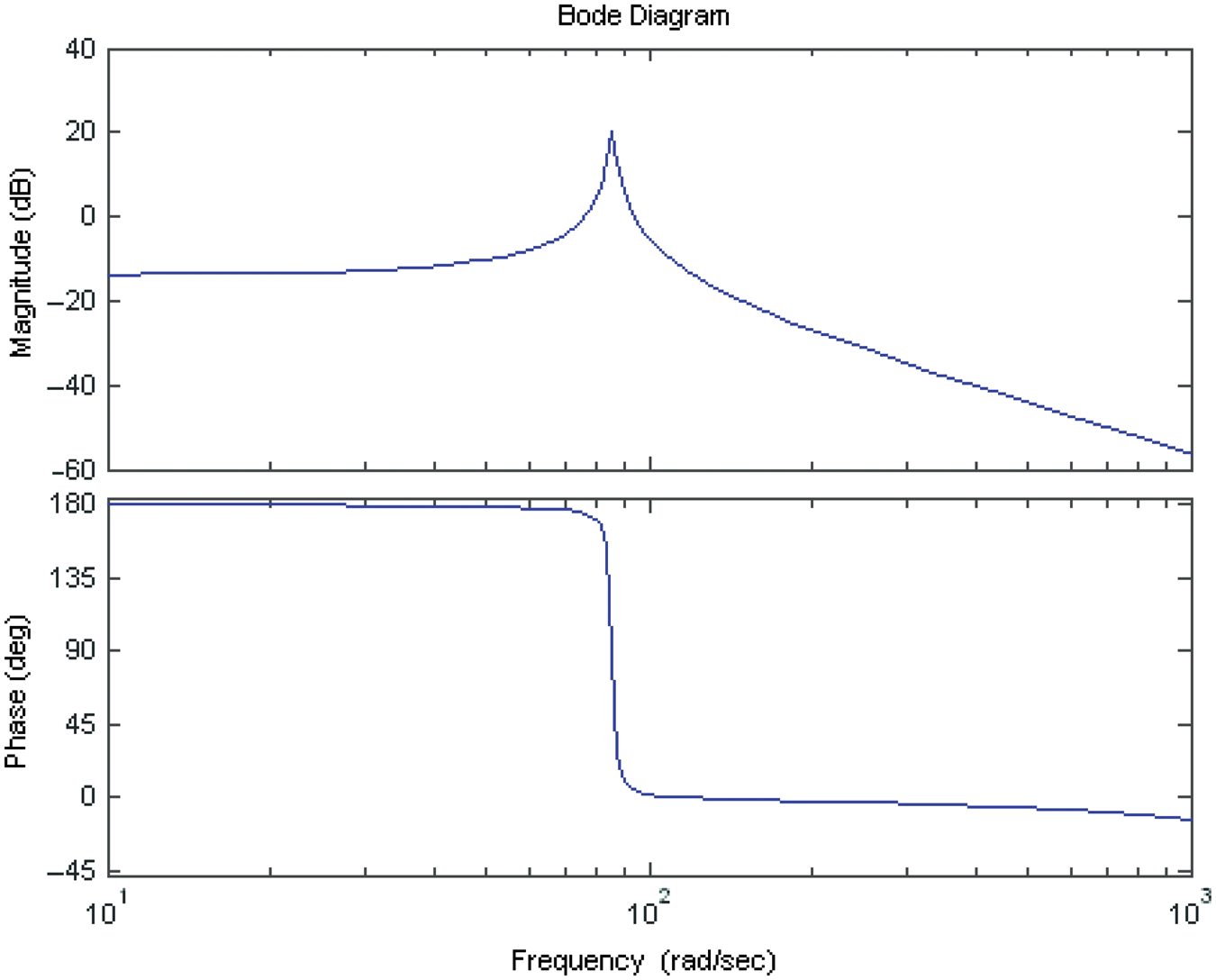
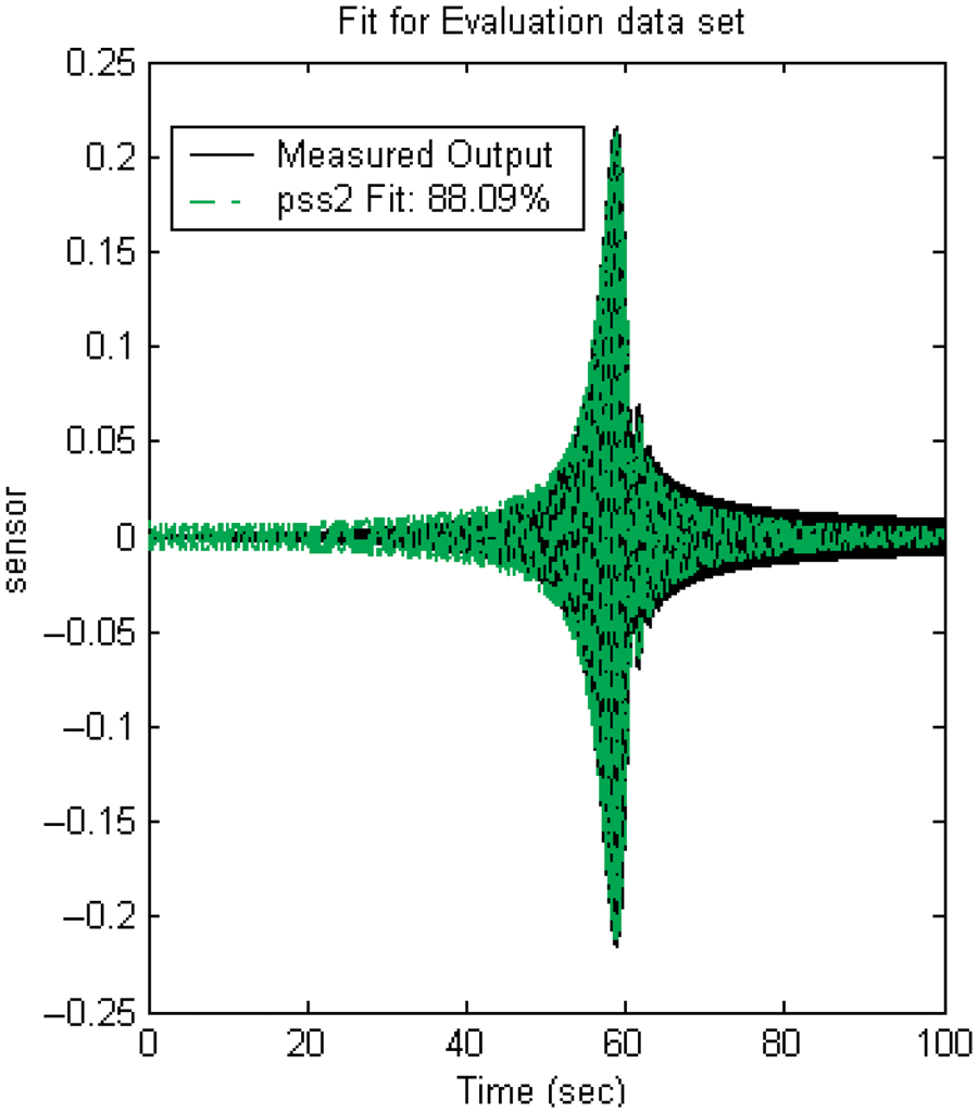
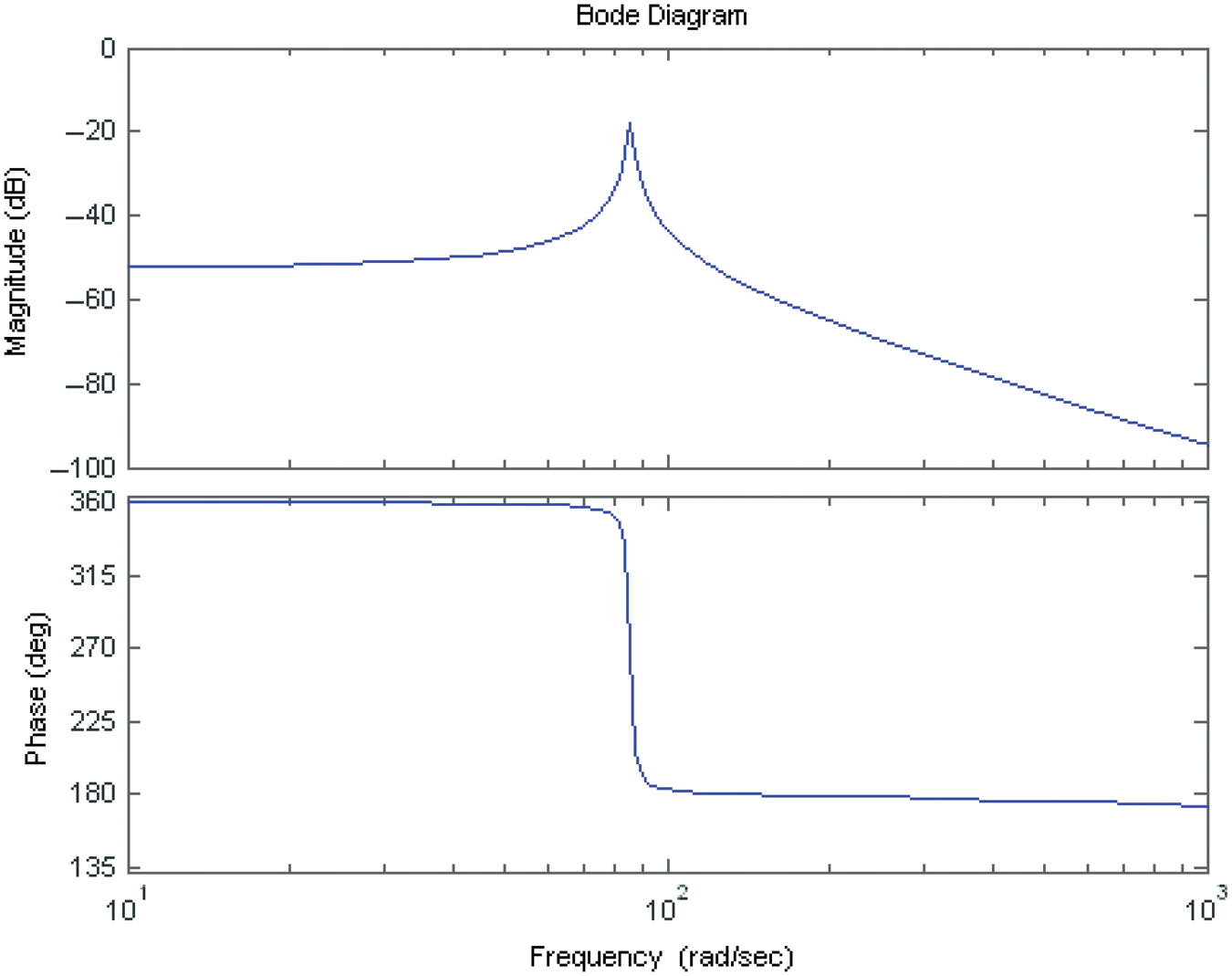
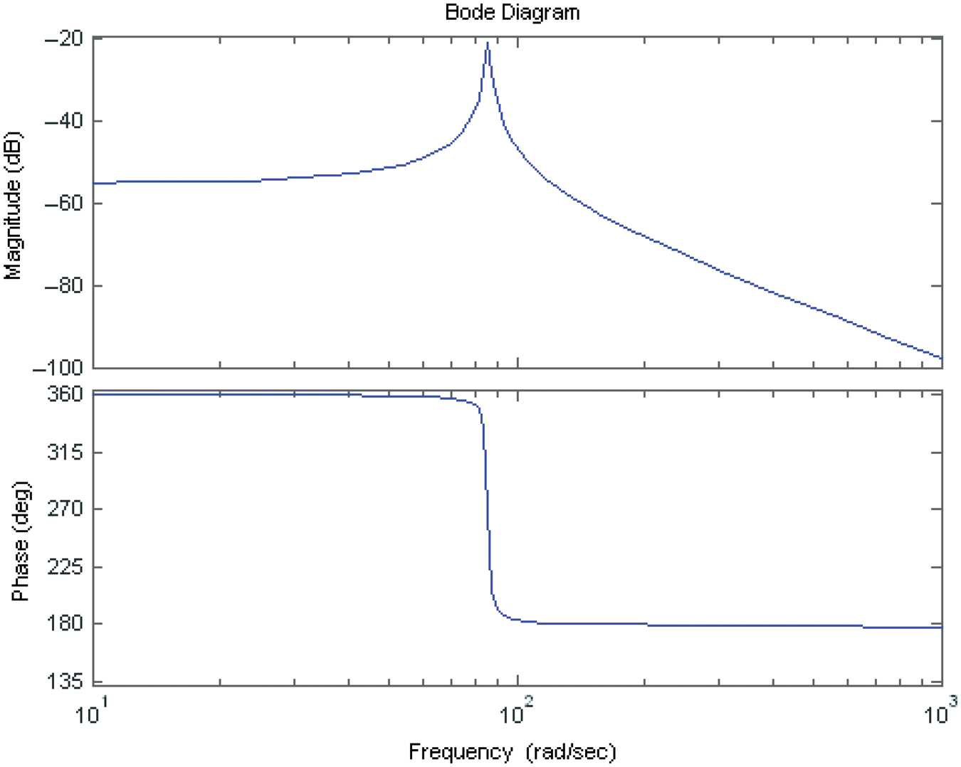
Using the truss structure discussed above, node 4 by a sweep sine signal of frequency ranging from 5 Hz to 20 Hz for 100 seconds. Using the MATLAB System Identification toolbox a state space model of second order is obtained. The validation results of the identified models from the shaker to sensors are shown from the Figures 9 to 12 with fits of 88.44%, 87.83%, 87.49% and 87.16%, respectively. The Bode plots of the identified model from Figures 13 to 16 clearly show the resonance frequency at 13.68 Hz (85.95 rad/sec).

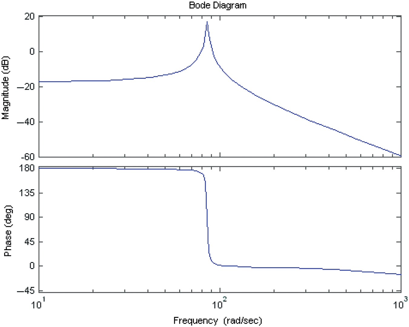
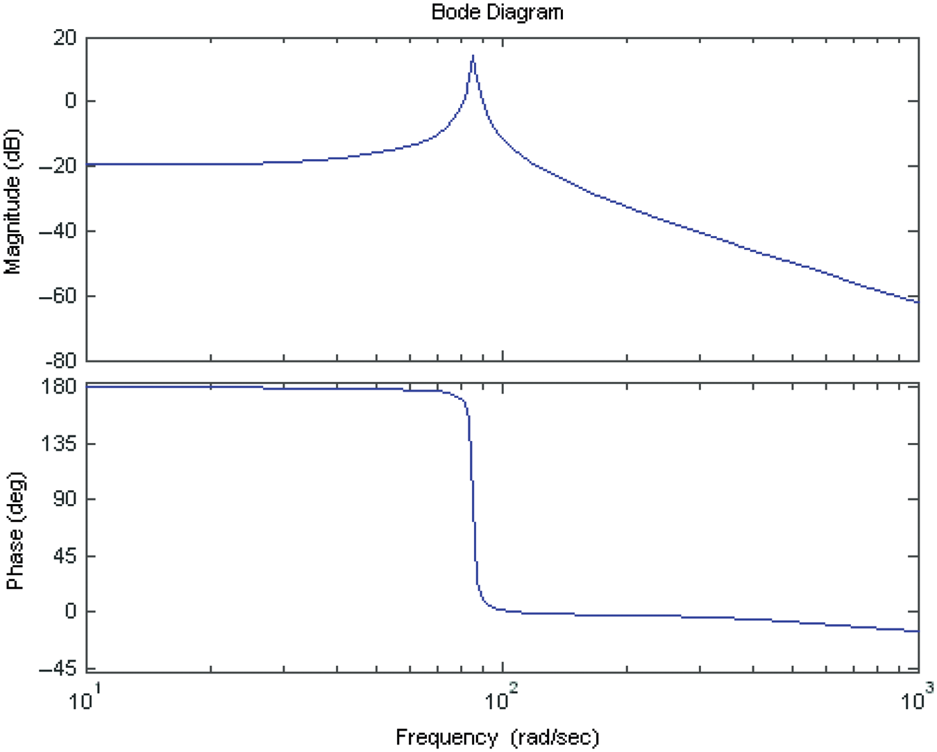
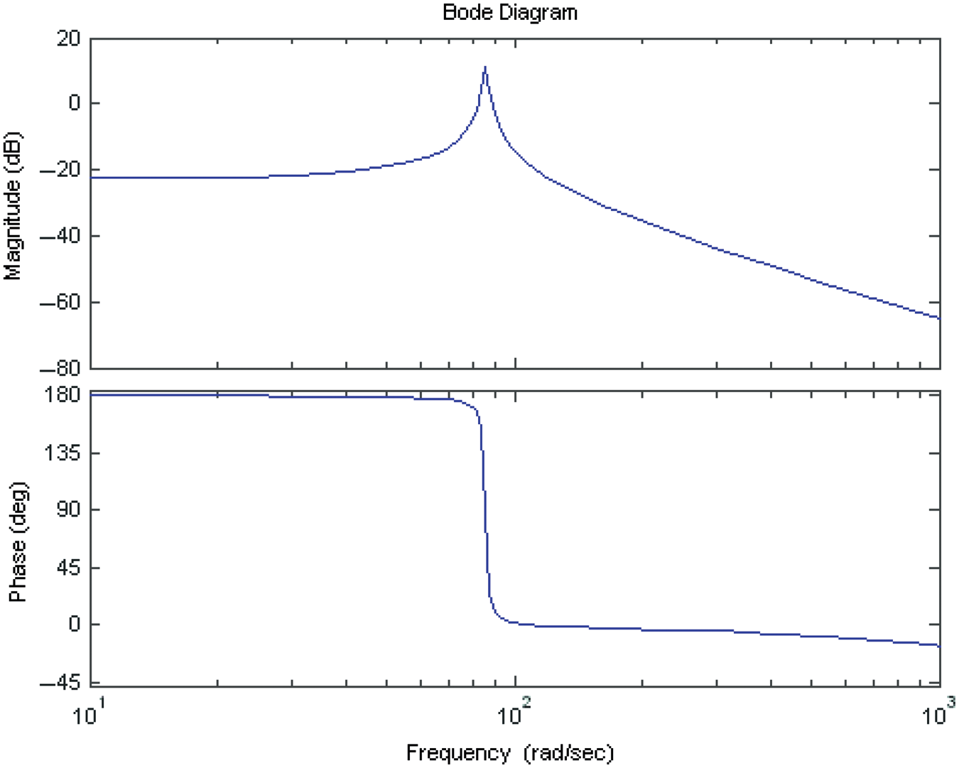
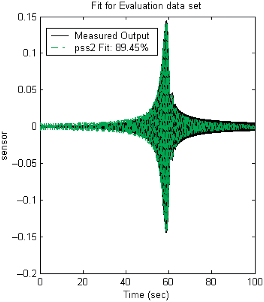
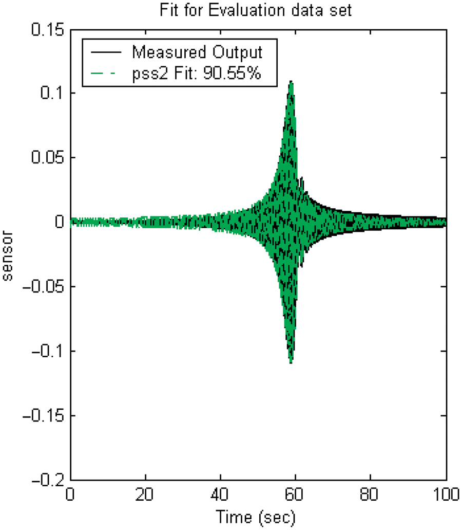
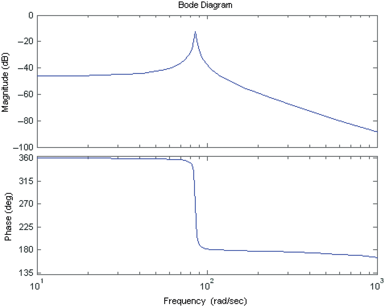
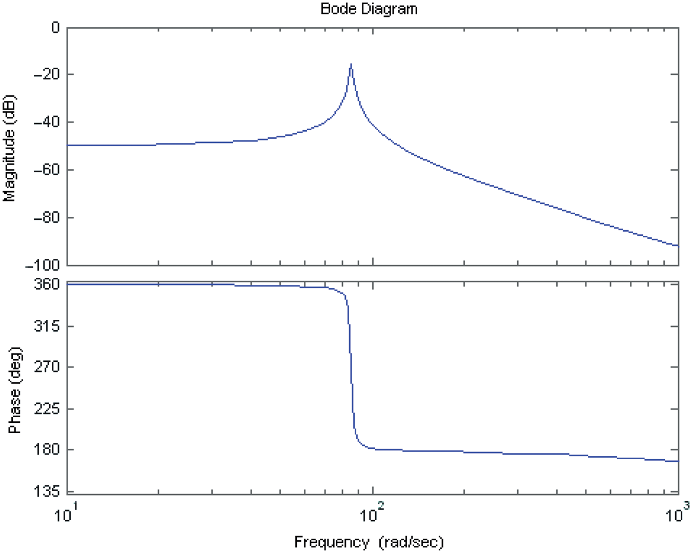
Similarly, the validation results of the identified models from the controllers to sensors are shown from the Figures 17 to 20 with fits of 88.09%, 89.45%, 90.55% and 92.21%, respectively. The Bode plots of the identified model are shown from Figures 21 to 24.

Figure 20.

Comparison of output and identified model (from controller to sensor 4).

Figure 21.

Bode diagram of identified model (from controller to sensor 1).

Figure 22.

Bode diagram of identified model (from controller to sensor 2).

Figure 23.

Bode diagram of identified model (from controller to sensor 3).

Figure 24.

Bode diagram of identified model (from controller to sensor 4).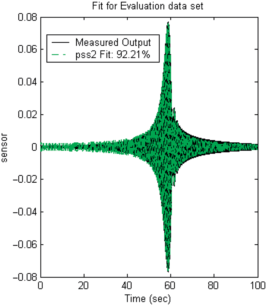

6. Design of the H∞ filter and fault tolerant H∞ controller

Some research on FTC turns to designing an integrated filter and controller. Such methods usually lead to high order integrated filter/controllers. To ease the implementation of the FTC, the H_∞ FDI filter and H_∞ FTC were designed separately.

6.1. Weight selection

In the literature regarding H_∞ norm analysis and design, the weight function selection is a highly problem-dependent, iterative process. Usually, the trial-and-error procedure is repeated until the desired performance and robustness objectives are achieved. In this research, the control objective is to suppress the first mode vibration of the smart structure. The disturbance input weight, W_d, is used to shape the worst case disturbance and can be a low pass shape or stress the amplitude at the frequency of the first mode. In this study, we use a sine wave with the frequency of the first mode of the structure as the disturbance input. The disturbance input weight is set to scalar 1. The performance or error weight, W_e, is used to specify the performance objectives of the resulting filter from the H_∞ optimization, e.g. bandwidth, steady-state requirements, and attenuation/amplification of signals at certain frequency ranges.Typically, the actuator fault input weight, W_f, has low-pass characteristics to emphasize the effects of faults on the low-frequency domain. Figure 25 shows the frequency responses of the designed weights.

Figure 25.

Weights design of fault detection and isolation and fault tolerant controller system.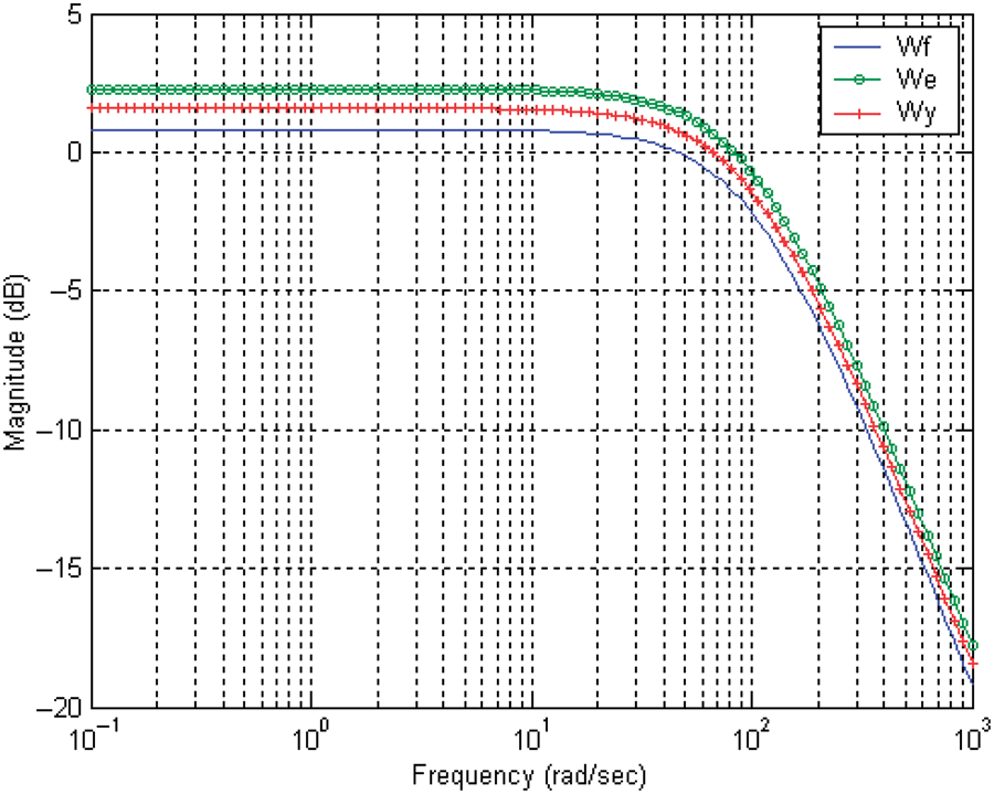

6.2. Fault tolerant controller design

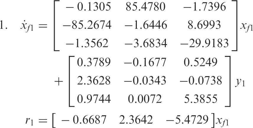
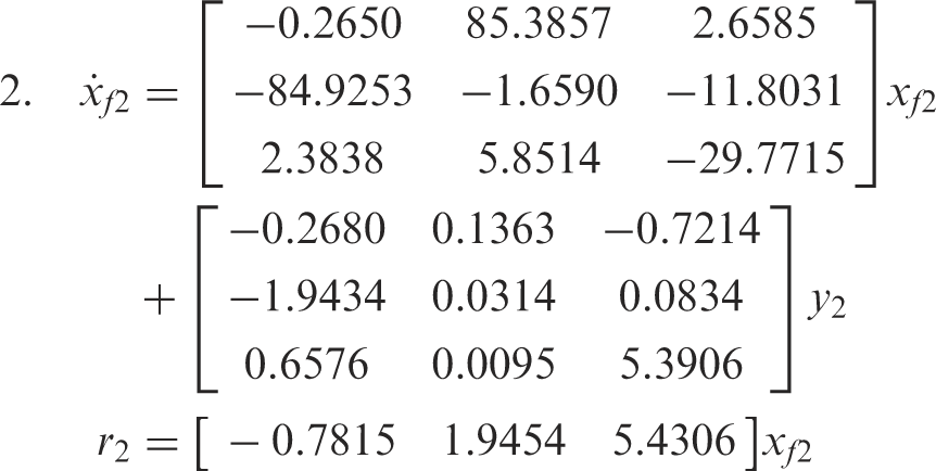
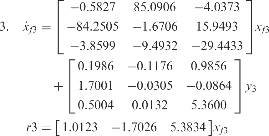
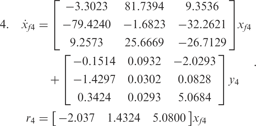
The identified structure model combined with the weights yields the augmented model, P, as shown in the bold black square in Figure 1. Using the developed LMI method, the following four stable, 3 rd order H_∞ filters for sensors are obtained:

\begin{matrix} 2 . {\overset{\cdot}{x}}_{f 2} = [\begin{matrix} - 0.265085.38572.6585 - 84.9253 - 1.6590 - 11.8031 2.38385.8514 - 29.7715 \end{matrix}] x_{f 2} \\ + [\begin{matrix} - 0.26800.1363 - 0.7214 - 1.94340.03140.0834 0.65760.00955.3906 \end{matrix}] y_{2} \\ 1.7 em r_{2} 1.7 em = [\begin{matrix} - 0.78151.94545.4306 \end{matrix}] x_{f 2} \end{matrix}

\begin{matrix} 3 . {\overset{\cdot}{x}}_{f 3} = [\begin{matrix} - 0.582785.0906 - 4.0373 - 84.2505 - 1.670615.9493 - 3.8599 - 9.4932 - 29.4433 \end{matrix}] x_{f 3} \\ + [\begin{matrix} 0.1986 - 0.11760.9856 1.7001 - 0.0305 - 0.0864 0.50040.01325.3600 \end{matrix}] y_{3} \\ 1.7 em r 31.7 em = [\begin{matrix} 1.0123 - 1.70265.3834 \end{matrix}] x_{f 3} \end{matrix}

\begin{matrix} 4 . {\overset{\cdot}{x}}_{f 4} = [\begin{matrix} - 3.302381.73949.3536 - 79.4240 - 1.6823 - 32.2621 9.257325.6669 - 26.7129 \end{matrix}] x_{f 4} \\ + [\begin{matrix} - 0.15140.0932 - 2.0293 - 1.42970.03020.0828 0.34240.02935.0684 \end{matrix}] y_{4} \\ 1.7 em r_{4} 1.7 em = [\begin{matrix} - 2.0371.43245.0800 \end{matrix}] x_{f 4} \end{matrix} .

Using a similar technique, the reduced 3 rd H_∞ controller is obtained.

6.3. Fault Detection and Isolation and Fault Tolerant Controller of the Truss Structure

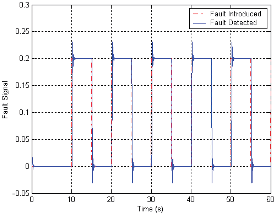
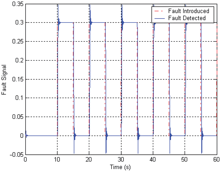
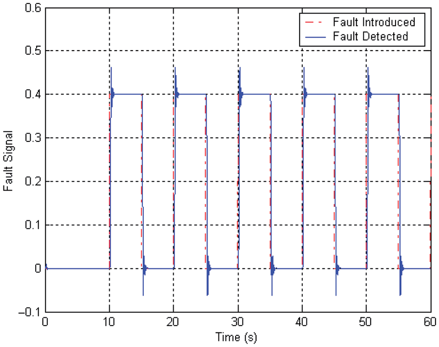
The truss was continuously excited by the sine wave at 85.95 rad/sec, the worst case disturbance input. The residual responses to different faulty inputs were examined. First, a faulty signal of square wave with varying amplitude was introduced into four sensors at time 10 sec. The filter outputs are shown in Figures 26 to 29. From these figures, we can see that the residual signal clearly identified the square wave.

Figure 26.

Fault identified in sensor 1.

Figure 27.

Fault identified in sensor 2.

Figure 28.

Fault identified in sensor 3.

Figure 29.

Fault identified in sensor 4.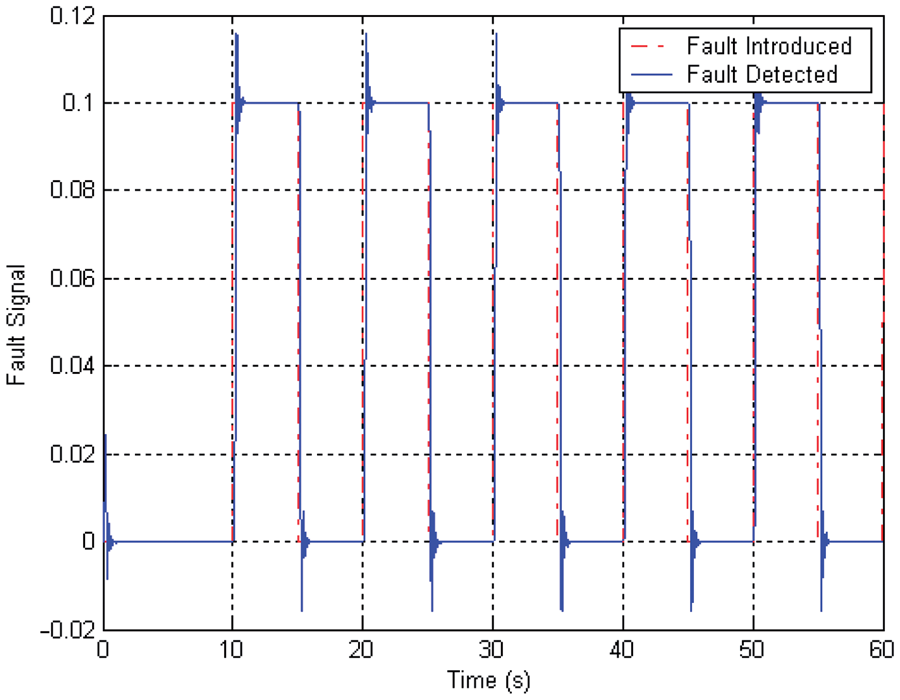

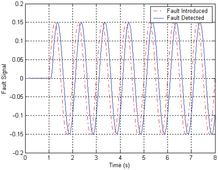
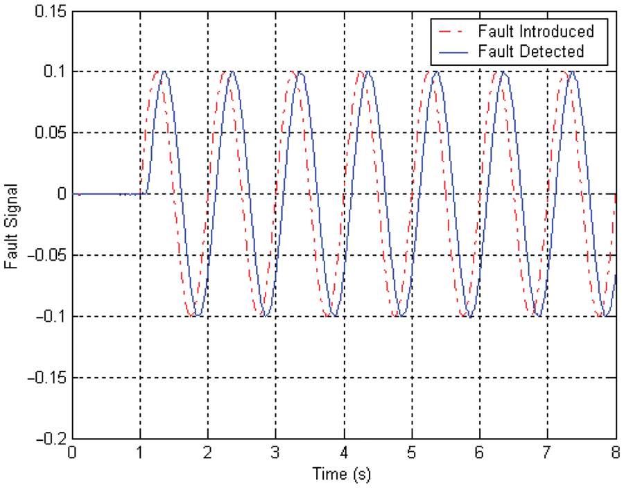
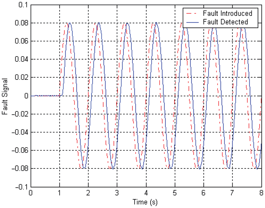
For comparison purposes, another simulation with sine wave faulty input was conducted. Figures 30 to 33 show the faulty input signal and the residual signal. It can be seen that within 1 second of the occurrence of the fault, the residual signal clearly indicated the fault.

Figure 30.

Fault identified in sensor 1.

Figure 31.

Fault identified in sensor 2.

Figure 32.

Fault identified in sensor 3.

Figure 33.

Fault identified in sensor 4.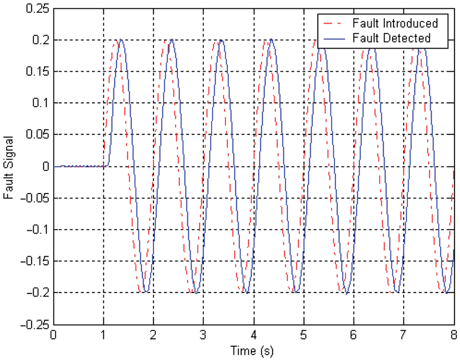

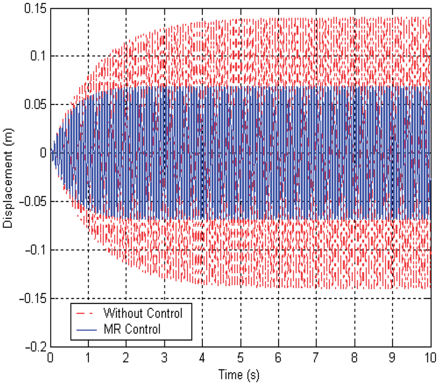
Next, the designed H_∞ FTC controller was examined in the MR damper. The structure was excited by a sine wave at 85.95 rad/sec. To simulate the partial failure of sensors, the outputs of the sensor 1, 2, 3 and 4 were reduced to 10%, 20%, 30% and 40% after 5 seconds had elapsed, respectively.

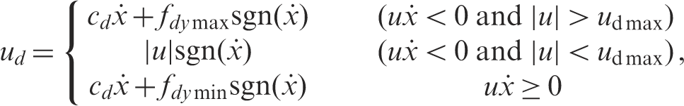
The semi-active control law of the MR damper is

u_{d} = {\begin{matrix} c_{d} \overset{\cdot}{x} + f_{dy max} sgn (\overset{\cdot}{x}) | u | sgn (\overset{\cdot}{x}) c_{d} \overset{\cdot}{x} + f_{dy min} sgn (\overset{\cdot}{x}) \end{matrix} \begin{matrix} (u \overset{\cdot}{x} <0 and | u | {>u}_{d max}) (u \overset{\cdot}{x} <0 and | u | {<u}_{d max}) u \overset{\cdot}{x} \geq 0 \end{matrix},

where u_d is the control force applied by the MR damper and u is the optimal force acquired by FTC. The parameters of the MR damper are

c_{d} = 2.8332 \times 10^{3} N \cdot s / m

and

f_{dy max} = 2.1875 \times 10^{3} N

. The displacement at the tip of the truss is shown in Figure 34. It can be seen that the response of the closed-loop system with the FTC controller is reduced by about 50%, though there are partial faulty signals in the outputs of sensors. The result of the FTC Controller without faults in sensors is shown in Figure 35. Comparing the two figures, it can be clearly seen that the system with FTC controller remained almost unchanged when there was a failure in the sensors.

Figure 34.

Displacement at tip of truss (with faults).

Figure 35.

Displacement at tip of truss (without faults).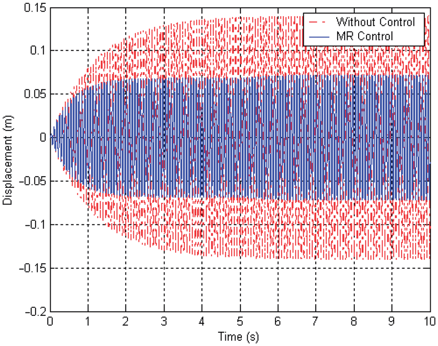

7. Conclusions

In this research, model-based FDI and the solution of the fault tolerant control problem using H_∞ techniques are considered for the vibration control of truss structures. An LMI formulation is obtained to design a full order robust H_∞ filter to estimate the faulty input signals. The FDI LMI synthesis conditions are obtained by applying the Bounded Real Lemma to the closed loop system. A feasible solution for these conditions forms a convex problem for the full order filter, which is solved via LMI optimization techniques. A fault tolerant H_∞ controller is designed for the combined system of plant and filter which minimizes the control objective selected in the presence of disturbances and faults. An 8-bay truss structure is used in validation of the FDI filter and FTC controller designs through numerical simulations. An MR damper is implemented in the truss to reduce the vibration of the truss using a FTC controller. To assist control system design, system identification is conducted for the first vibration mode of the truss. The state space model from system identification is used for the H_∞ filter design. The residuals obtained from the filter through simulation are seen following the faults signals. The result shows that the designed FTC controller can achieve effective vibration reduction, though there are partial faulty signals in the outputs of sensors. The numerical simulation results have demonstrated the proposed FDI and FTC in dealing with the faults of sensors of the semi-active control system, however, it is still necessary to experimentally verify the effectiveness of proposed method. The experimental study on the FDI and FTC of truss structures using MR dampers are considered as a future work.

Footnotes

Acknowledgements

LH and GS are grateful for the support of their funding bodies.

Funding

This work was supported by Institute of Space Systems Operations (ISSO) at University of Houston, National Earthquake Special Founding of China (grant number 200808074) and National Natural Science Foundation of China (grant number 50708016 and 51121005).

References

Bai

(2006) Advanced controls of large scale structural systems using linear matrix inequality methods. PhD thesis, University of Houston, Texas.

Bai

Grigoriadis

(2005) H∞ collocated control of structural systems: an analytical bound approach. Journal of Guidance, Control, and Dynamics 28(5): 850–853.

Boyd

Ghaoui

Feron

Balakrishnan

(1994) Linear Matrix Inequalities in Systems and Control Theory. Philadelphia: Society for Industrial Mathematics.

Chen

Nagarajaiah

(2007) Linear matrix inequality based robust fault detection and isolation using the eigenstructure assignment method. Journal of Guidance, Control, and Dynamics 30(6): 1831–1835.

Chen

Nagarajaiah

(2008) H_/H_inf structural damage detection filter design using iterative LMI approach. Smart Materials and Structures 17(3): 035019–035019.

Chen

Patton

(1999) Robust Model-Based Fault Diagnosis for Dynamics Systems. London: Kluwer Academic Publishers.

Diallo

Benbouzid

MEH

Makouf

(2004) A fault-tolerant control architecture for induction motor drives in automotive applications. IEEE Transactions on Vehicular Technology 53(6): 1847–1855.

Douglas

Speyer

(1999) H∞ bounded fault detection filter. Journal of Guidance, Control and Dynamics 22(1): 129–138.

Dyke

Spencer

(1997) Comparison of semi-active control strategies for the MR damper. In Proceedings of Intelligent Information Systems. Washington DC: IEEE Computer Society, December 8–10, pp. 580–584.

10.

Dyke

Spencer

Sain

Carlson

(1996) Modeling and control of magnetorheological dampers for seismic response reduction. Smart Materials and Structures 5(5): 565–575.

11.

Eryurek

Upadhyaya

(1995) Fault-tolerant control and diagnostic for large-scale systems. IEEE Control System Magazine 15(5): 34–42.

12.

Gahinet

Apkarian

(1994) A linear matrix inequality approach to H∞ control. International Journal of Robust and Nonlinear Control 4(4): 421–448.

13.

Geromel

Peres

PLD

Souza

(1996) Convex analysis of output feedback control problems. IEEE Transactions on Automatic Control 41(7): 997–1003.

14.

Grigoriadis

(1995) Optimal H∞ model reduction via linear matrix inequalities: Continuous- and discrete-time cases. Systems and Control Letters 26(5): 321–333.

15.

Grigoriadis

Skelton

(1996) Low-order control design for LMI problems using alternating projection methods. Automatica 32(8): 1117–1125.

16.

Grigoriadis

Skelton

(1998) Integrated structural and control design for vector second-order systems via LMIs. In Proceedings of the 1998 American Control Conference, Washington DC. June 21–26 pp. 1625–1629.

17.

Hamouli

Sauter

Keller

(2004) Fault Tolerant control using augmented fault detection filter. In: Proceedings of 2004 IEEE International Symposium on Industrial Electronics, Washington, DC. May 4–7 pp. 109–114.

18.

Iwasaki

Skelton

(1994) All controllers for the general H∞ control problem: LMI existence conditions and state space formulas. Automatica 30(8): 1307–1317.

19.

Koh

Dharap

Nagarajaiah

Phan

(2005a) Real-time structural damage monitoring by input error function. Journal of American Institute of Aeronautics and Astronautics 43(8): 1808–1814.

20.

Koh

Dharap

Nagarajaiah

Phan

(2005b) Actuator failure detection through interaction matrix formulation. Journal of Guidance, Control, and Dynamics 28(5): 895–901.

21.

H-N

Chang

Z-G

Song

(2005) Studies on structural vibration control with MR dampers using µGA. Earthquake Engineering and Engineering Vibration 4(2): 301–304.

22.

Song

(2010) A genetic algorithm-based two-phase design for optimal placement of semi-active dampers for nonlinear benchmark structure. Journal of Vibration and Control 16(9): 1379–1392.

23.

Koh

Nagarajaiah

(2007) Detecting sensor failure via decoupled error function and inverse input-output model. Journal of Engineering Mechanics 133(11): 1222–1228.

24.

Liu

Song

(2007) Non-model based semi-active vibration suppression of stay cables using magneto-rheological (MR) fluid damper. Smart Materials and Structures 16: 1447–1452.

25.

Ljung

(1999) System Identification: Theory for the User. Upper Saddle River NJ: Prentice Hall Inc.

26.

Mahmoud

Jiang

Zhang

(2003) Active Fault Tolerant Control Systems. New York: Springer.

27.

Maki

Jiang

Hagino

(2001) A stability guaranteed active fault tolerant control system against actuator failures. In: Proceedings of the 40th IEEE Conference on Decision and Control, Washington DC. December 4–7 pp. 1893–1898.

28.

Narasimhan

Suresh

Nagarajaiah

Sundararajan

(2008) On-line learning failure-tolerant neural-aided controller for earthquake excited structures. Journal of Engineering Mechanics 134(3): 258–268.

29.

Onoda

(2002) An experimental study of a semiactive magneto-rheological fluid variable damper for vibration suppression of truss structures. Smart Materials and Structures 11(11): 156–162.

30.

Skelton

Iwasaki

Grigoriadis

(1998) A Unified Algebraic Approach to Linear Control Design. London: Taylor & Francis.

31.

Sodeyama

Sunakoda

(2003) Dynamic tests and simulation of magneto-rheological dampers. Computer-Aided Civil and Infrastructure Engineering 18(1): 45–57.

32.

Song

Vllatas

Johnson

Agrawal

(2002) Active vibration control of a space truss using piezoceramic stack actuator. Journal of Aerospace Engineering 215, Part G.

33.

Spencer

Dyke

Sain

Carlson

(1997) Phenomenological model for magnetorheological dampers. Journal of Engineering Mechanics 123(3): 230–238.

34.

Spencer

Yang

Carlson

Sain

(1998) Smart dampers for seismic protection of structures: a full-scale study. In: Proceedings of the 2nd World Conference on Structural Control, Mississauga, Canada, June 28 – July 1 pp. 417–426.

35.

Wang

Song

(2011) Fault detection and fault tolerant control of a smart base isolation system with magneto-rheological damper. Smart Materials and Structures 20: 085015–085015.