
Abstract
The dynamical model of a flexible Euler–Bernoulli link system subject to high-speed motions is developed. Nonlinear kinematics are considered to take into account the foreshortening effect of the link. A continuous model with boundary conditions is derived using Hamilton's principle and spatially discretized dynamical equations are derived using Lagrange's equation based on the expression of the kinetic and potential energies of the flexible link system. The effect of the links foreshortening on the dynamical response is shown for a sinusoidal torque input at the links hub. The simulation results showed that for small torque amplitudes the difference between linear and nonlinear kinematics is small. However, for large amplitudes, this difference is prominent.
1. Introduction
In manufacturing and space applications, the use of lightweight structures in robot manipulators is motivated by their capacity for high-speed maneuvers, their high payload-to-arm-weight ratio, higher mobility, reduced energy consumption, and lower inertia forces for accurate positioning. It is also advantageous to use thin and flexible links in surgical robotics for minimal invasiveness (Tavakoli and Howe, 2009). To ensure satisfactory performances of such systems, their flexibility should be included in modeling and in control design. This flexibility becomes more significant in cases of larger structures and more stringent performance demands.
In modeling flexible links manipulators, the most widely used methods to develop manipulators dynamics are based on energy principles such as Hamilton's principle (Cetinkunt and Yu, 1991; Junkins and Kim, 1993) and Lagrange's equations (Book, 1984; De Luca and Siciliano, 1991). Energy principle-based models of flexible manipulators are spatially continuous of infinite order. To generate spatially discrete models the assumed-mode method (AMM) or the finite-element method (FEM) are generally used. The accuracy of the dynamical model obtained from the analytical formulation is highly dependent on the adopted mode shapes of links deflections and their number. For high-speed maneuvers, it is also dependent on the foreshortening effects of the links, i.e. the axial displacement due to bending deformation of the links, by considering a linear first-order or a nonlinear second-order kinematics.
Static and dynamic analysis of flexible manipulators have been the subject of many investigations. In particular, different comparisons have been devoted to the study of the effectiveness and accuracy of spatially discretized models. Recently, the dynamics of a flexible-hub geometrically nonlinear beam carrying a tip mass was presented in (Emam, 2010). The hub–beam system is assumed to move in plane and the hub is restrained by a vertical translational movement and a rotational spring. The dynamical responses of the system with one, two, and three modes show the effect of the number of modes on the dynamical response. Saad et al. (2006) presented a detailed comparison between assumed-based models and finite-element ones for a single flexible link system for one to eight flexible modes. This comparison shows that clamped beam shape functions for the AMM, and cubic splines finite elements for the FEM describe the shape functions of flexible links best.
A common way to describe a flexible link is by means of the Euler–Bernoulli equation. This model is valid under the assumptions that: (i) the link is slender with uniform geometric and inertial characteristics, (ii) the link is flexible in the lateral directions and stiff with respect to axial forces and to torsion and bending forces due to gravity, and (iii) nonlinear deformation and friction can be neglected. The Euler–Bernoulli beam with linear kinematics is a linear infinite-dimensional model which takes into account only perpendicular deformation with respect to an unstressed reference configuration. For high-speed maneuvers, however, nonlinear kinematics that take into account foreshortening effects of a flexible link are to be considered (Boyer et al., 2002).
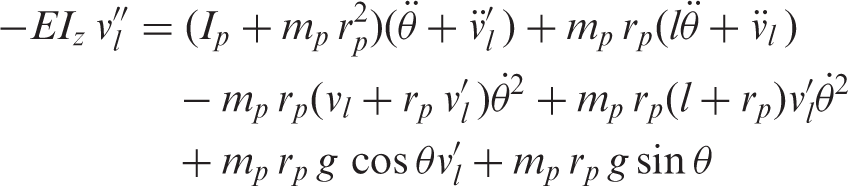
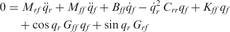
Owing to the assumption of small deformation, the Euler–Bernoulli beam model of a single flexible link system is linear in the link deformation, see Cannon and Schmitz (1984), Cetinkunt and Yu (1991), and Jnifene (2007), to name a few. This assumption implies a first-order approximation of the deformation in the final dynamical model. The energy expressions are, however, nonlinear. To consider a nonlinear model, quadratic terms in the deformation are considered, particularly in the mass matrix M(v2), where v is the link's deformation at a point along its axis (Yung and Chen, 1990; Yim et al., 1992; Zaad and Khorasani, 1996; Geniele et al., 1997; Lee, 2005). Coriolis and centrifugal terms are also added such that
Al-Bedoor and Hamdan (2001) developed a nonlinear model for a flexible link moving in the horizontal plane. They consider the foreshortening effect by considering a fourth-order kinematics. The resulting model is well suited for simulation. For control purposes, however, particularly in robotics, Euler–Bernoulli beams are often used to describe flexible links where links deformation is considered to be small relative to their length. A second-order kinematics is largely sufficient for robotics applications with high-speed maneuvers.
Cai et al. (2005) developed a nonlinear model for a single flexible link system taking into account foreshortening effects. A second-order kinematics was considered for the large motion at high speed. A spatially discretized model was also developed using Hermite cubic finite elements. However, the frequencies of the resultant model do not converge monotonically from above when the number of elements is increased (Meirovitch and Silverberg, 1983)
The objective of this work is to develop a nonlinear dynamical model of a one flexible link system. The systems movement is not restricted to the horizontal plane, but considered in the vertical one. The horizontal plane dynamic becomes a special case of the vertical one. An analytical continuous dynamical model is developed using Hamilton's principle. A spatially discrete dynamical model is given using Lagrange's equations with the AMM. In contrast to Cai et al. (2005), the resultant frequencies in the AMM model are known to be convergent from above when the number of modes is increased. The rotating beam eigenfunctions are also developed for the linearized system. The developed nonlinear dynamical model is particularly useful for nonlinear control purposes. The deformations are assumed to be small while the speed of the motion is considered to be high. We consider the foreshortening effect of the link by considering second-order nonlinear kinematics. The effect of the foreshortening is shown by simulating the response of the developed dynamics to various sinusoidal inputs.
Section 2 describes the features of the flexible link system under consideration and presents its continuous model. The eigenvalue problem (EVP) and the discretized model are presented in Sections 3 and 4, respectively. Section 5 deals with the analytical aspects of the shape functions. The effect of the link foreshortening is shown by simulation in Section 6. A conclusion is presented in Section 7.
2. The continuous model
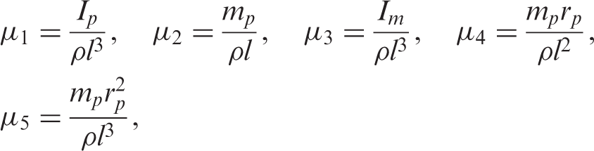
Figure 1 shows the one link flexible system. It consists of a motor, a flexible beam, and a payload. The motor has an angular position θ(t), a viscous friction b
m
, an inertia I
m
, and develops a torque T
m
. The beam length is l, its linear density ρ, its rigidity EI
z
, and its internal damping coefficient κ
e
. The payload has a mass m
p
, an inertia I
p
, and a center of mass r
p
. We assume that the system parameters are known. The gravity acts along the x-axis of frame ( A flexible rotating beam.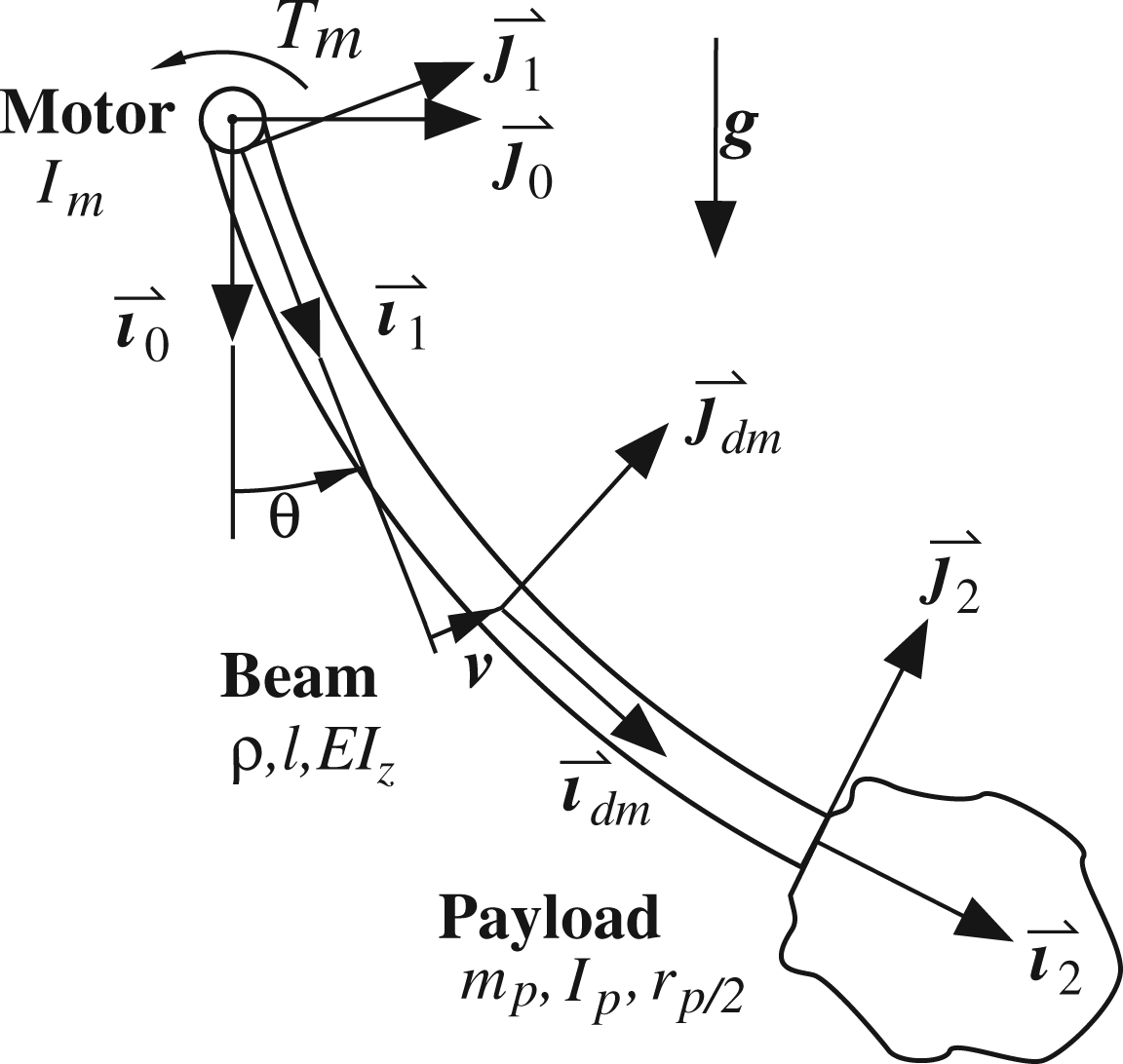
The continuous model consists of one ordinary differential equation (ODE) for the motor's motion, and a partial differential equation (PDE) with four associated boundary conditions (BCs) for the flexible link.
2.1. Kinematics
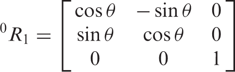
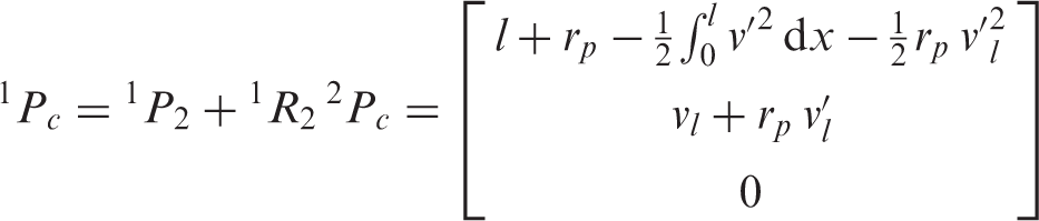
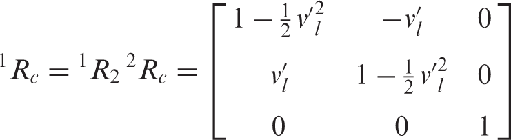
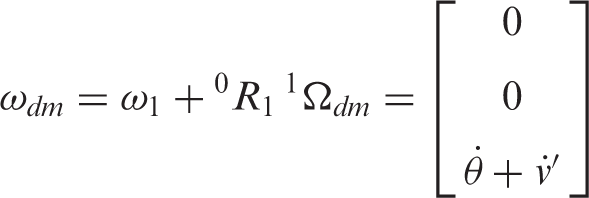
The position of reference frame ℛ1 relative to the inertial reference system ℛ0 is  2(v) term is a second-order term in v. This term is to be neglected if first-order kinematics was considered. The rotation matrix of ℛ
dm
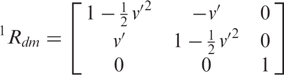
relative to ℛ1 is (Piedbœuf, 1998):
2(v) term is a second-order term in v. This term is to be neglected if first-order kinematics was considered. The rotation matrix of ℛ
dm
relative to ℛ1 is (Piedbœuf, 1998):
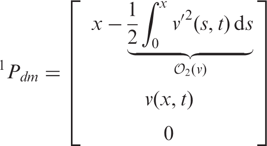
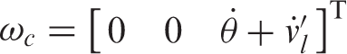
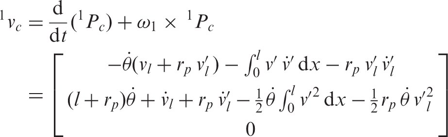
The position vector of the payload center of mass relative to ℛ1 is:
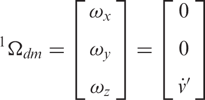
The angular velocity of ℛ1 relative to ℛ0 is

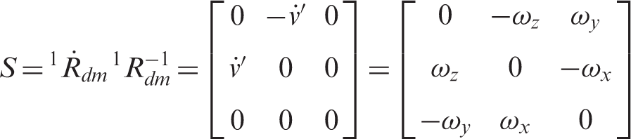
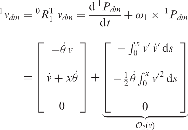
Using the antisymmetric matrix to represent the velocity of an element dm of the link:
The linear velocity of the origin of ℛ
dm
relative to ℛ0 is

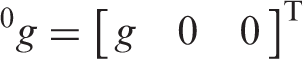
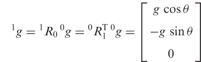
The gravity vector is represented in ℛ0 by
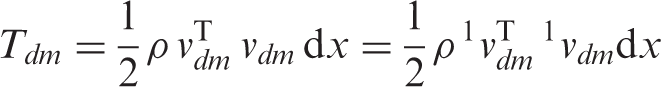
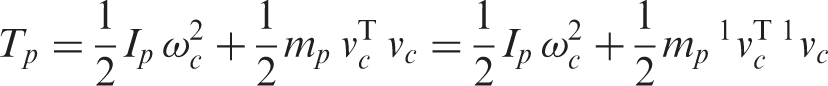
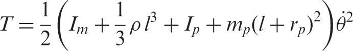
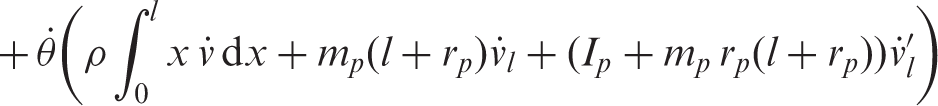
2.2. Kinetic energy
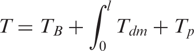
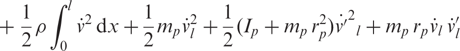
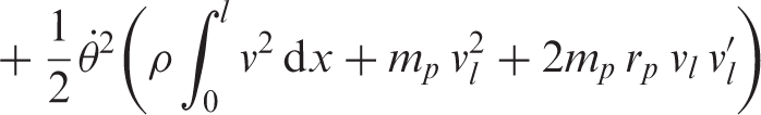
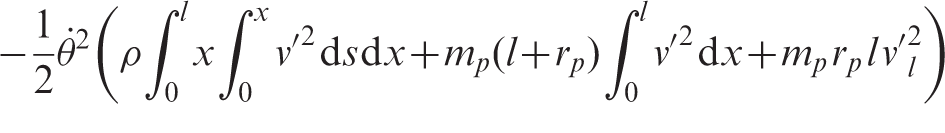
The kinetic energy of the given system is given by
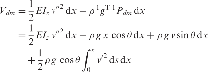
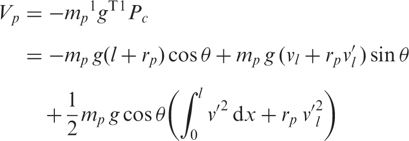
2.3. Potential energy
The potential energy of the given system is given by
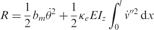
2.4. Rayleigh dissipation function
Friction is due to the motor's viscous friction and the link's internal damping. The Rayleigh dissipation function is then given by
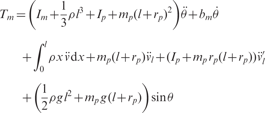
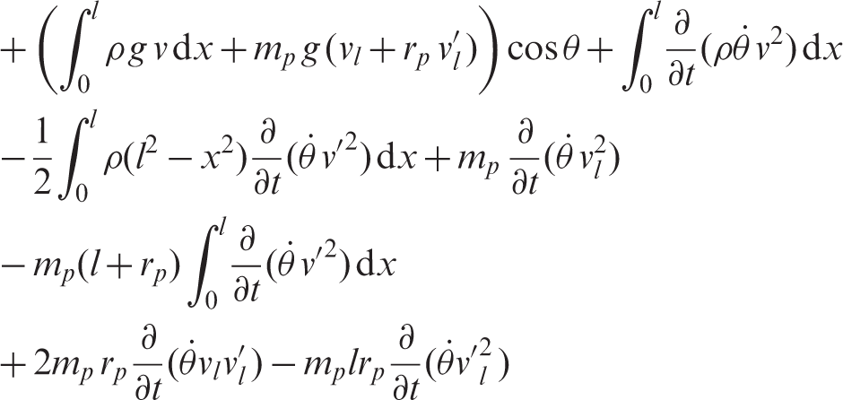
2.5. Dynamics
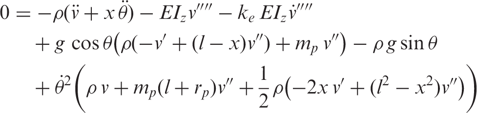
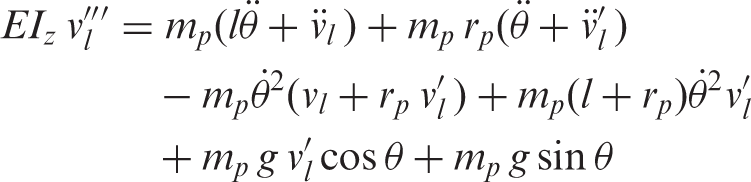
To develop the dynamics of the given system, we apply Hamilton's principle using the developed kinetic and potential energies. The variational of these expressions are simplified using integration by parts. First we ignore damping forces. The only nonconservative applied force is the motor torque T m . Two dynamical equations are then obtained. The first is associated with the motor's angle θ, and the second is associated with the deformation of the link v. Moreover, four BCs are associated with the dynamical equation of the deformation. These conditions describe the way in which the arm is attached to the base (geometrical BCs) and to the payload (natural BCs).
To complete these dynamics, we then add the viscous friction at the base and the link's internal damping. To take into account the friction at the base, the motor torque T
m
is replaced by


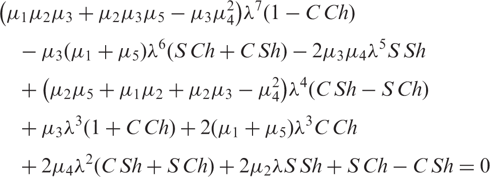
3. Eigenvalue problem
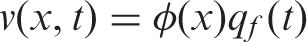
The EVP consists of solving for the deformation v the dynamics of the system represented by the ODE (5) and the PDE with the associated BCs (6)–(9). Let us consider the case of a homogeneous problem where the motor's torque is null, i.e. T
m
= 0. We consider a solution for v separable in space and time. The deformation is then given by
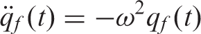
The EVP thus amounts finding one ω and a nontrivial solution φ(x) that verifies homogeneous discretized equations together with the associated BCs. The corresponding ω are the characteristic values or the eigenvalues and the φ(x) are the eigenfunctions. EVP generally generates the solution of a characteristic equation having an infinite countable number of solutions w r . For each eigenvalue w r corresponds an eigenfunction φ r (x). In the general case where dynamics is represented by nonlinear equations and with nonuniform parameters, a solution of the EVP is practically not possible. Approximate methods are used to solve this kind of problem (Mirovitch, 1967).
4. Spatial discretization
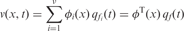
The order of the solution is infinite. In order to analyze and control this system, a spatially discrete model of finite order is suitable. A finite number of terms is then retained in the discretization of the deformation which is rewritten in the form:
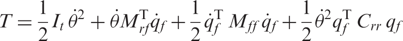
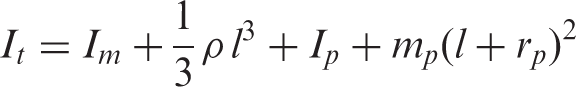
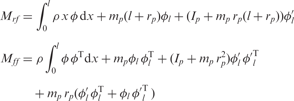
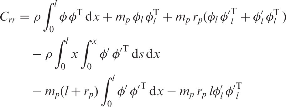
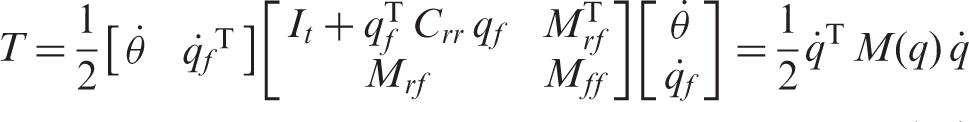
In the mass matrix M(q), the second-order element in v, i.e.
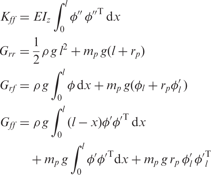
The discretization of the potential energy (3) gives

The discretization of the Rayleigh dissipation function (4) gives

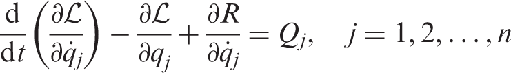
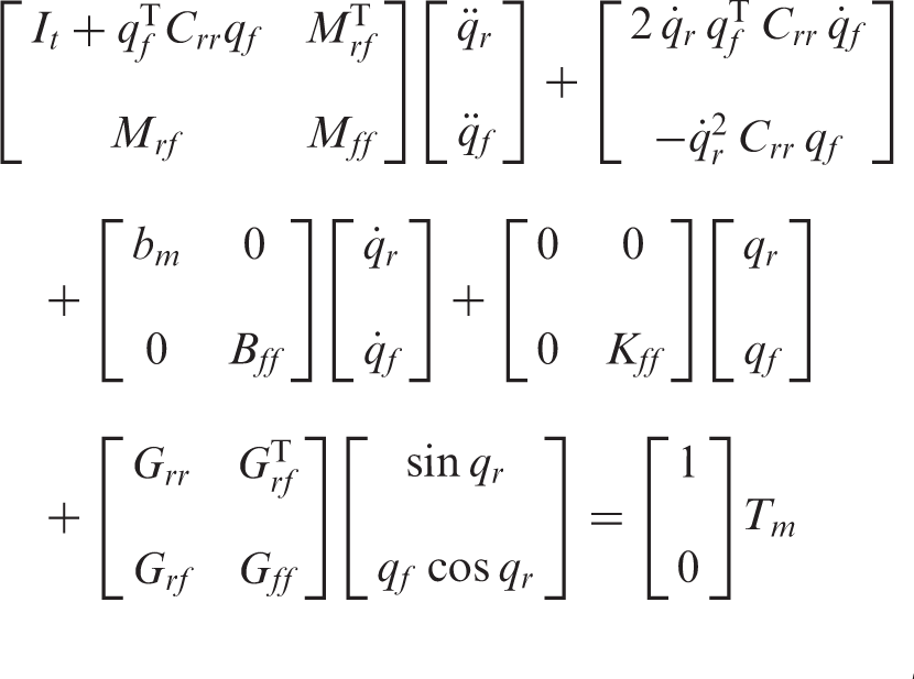
We then introduce these expressions into the Lagrangian ℒ = T − V and apply Lagrange equations:


Remark 1.
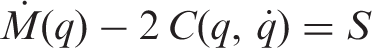
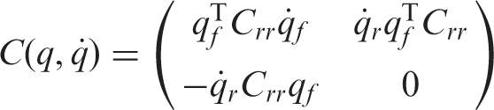
The mass matrix M and the Coriolis and centrifugal force vector
Let

By neglecting the second-order elements (relative to v) in (20), i.e. in the mass matrix and the gravity element G
ff
, equation (20) becomes

Remark 2.
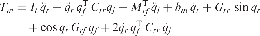
Nonlinear models are considered in the literature by considering the nonlinear element in the mass matrix, which is a second-order element in v. However, as shown in the dynamical equations (20), Coriolis nonlinear terms are also to be considered when a second-order term in v is to be considered. Actually, the amplitude of the nonlinear Coriolis elements is greater than the nonlinear mass element. The latter is small due to the hypothesis of small deformation. However, the Coriolis nonlinear elements are not eliminated by this hypothesis, they are the result of the multiplications of v and
5. Description of admissible functions
The analytical solution of the eigenfunctions of the system shown in Figure 1 is given by (Saad et al., 2006):
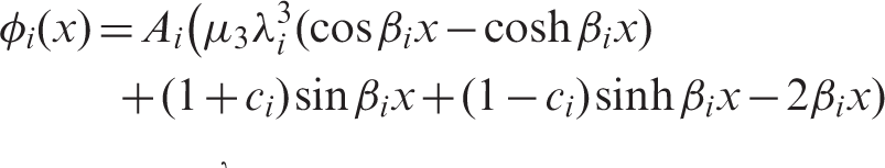
Here,

The admissible shape functions are generally the eigenfunctions of a simpler but related problem. The eigenfunctions of a rotating beam with a payload concentrated at its end (bp) are obtained from (24) and (25) by replacing the payload center of mass r
p
by zero. The eigenfunctions of a clamped beam with a concentrated payload (cp) are deduced from the bp eigenfunctions by taking the motor inertia I
m
as infinity. The eigenfunctions of a clamped–free beam (cf) are deduced from the cp ones by taking the payload inertia I
p
and mass m
p
as zero. The first four eigenfunctions of a rotating beam are shown in Figure 2.
First four eigenfunctions of a rotating beam.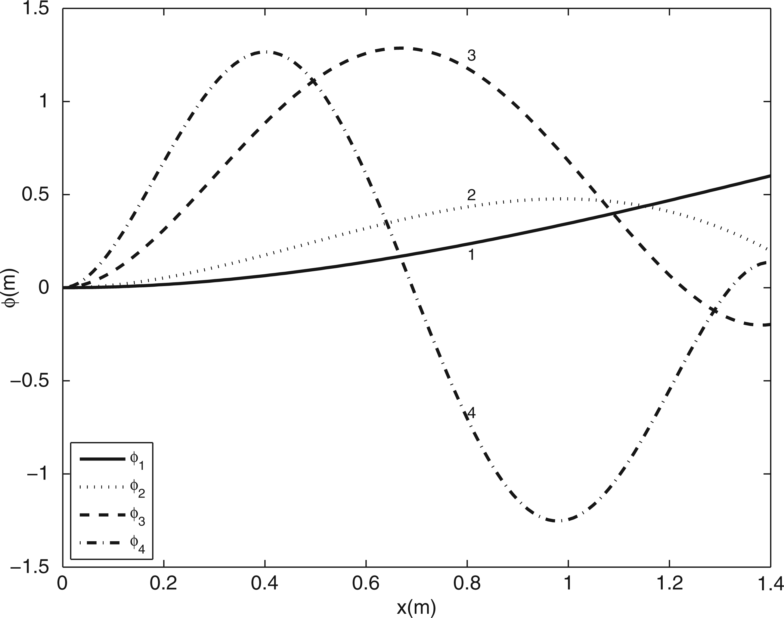
6. Simulations
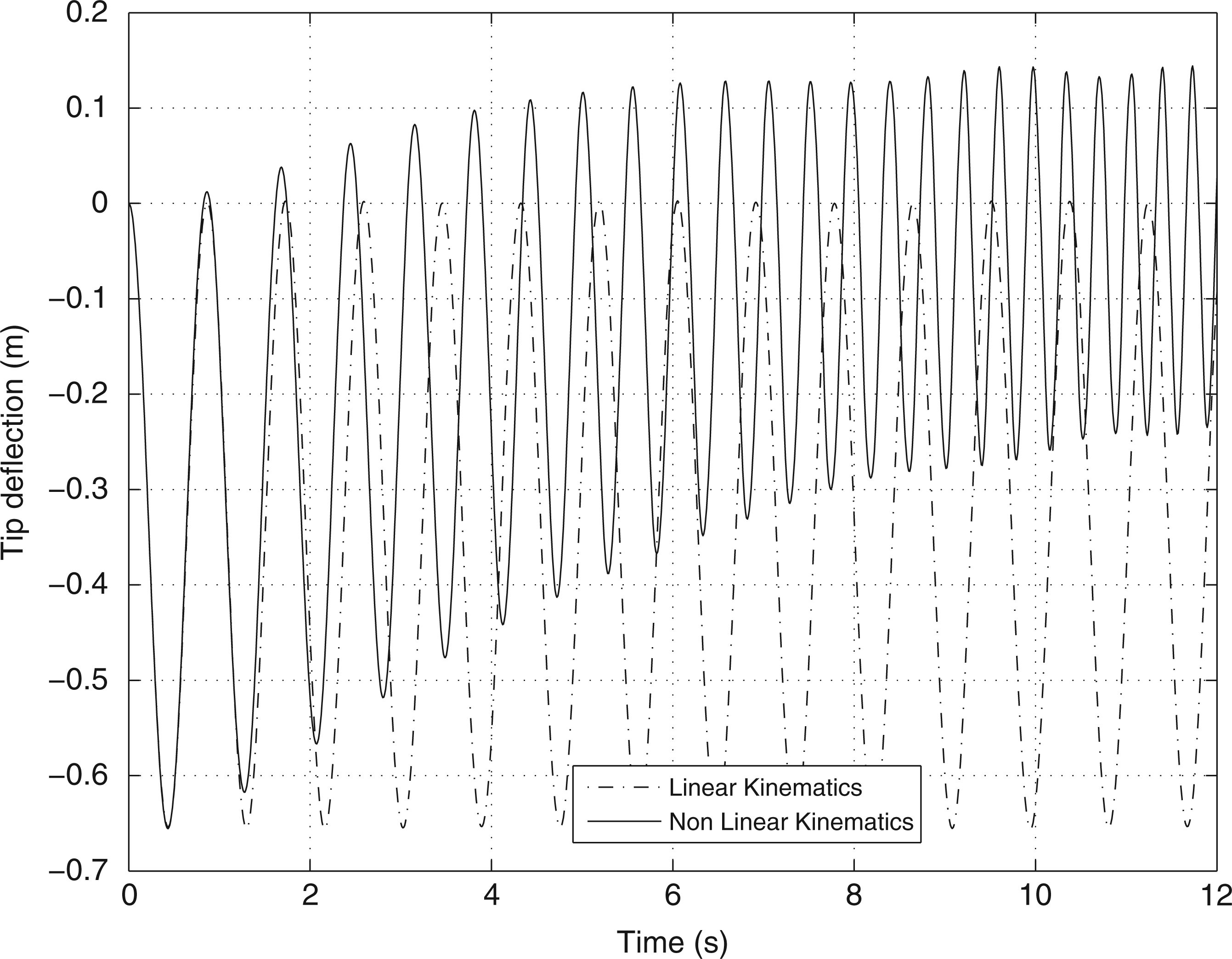
To show the foreshortening effects on the system's response, a sinusoidal torque input is applied to the system shown in Figure 1. For the sake of comparison with published results, the system is considered moving in the horizontal plane, i.e. gravity is eliminated (g = 0). The system's parameters are (Emam, 2010): the hub rotary inertia is J = 0.30 kg m2, the beam length is l = 1.8 m, the cross-sectional area is A = 2.5 × 10⁻⁴ m2, the area moment of inertia is I = 1.3021 × 10⁻¹⁰ m4, the mass density is ρ = 2.766 × 10³ kg/m3, the modulus of elasticity is E = 6.90 × 10¹⁰ N/m2, and the tip mass is m
p
= 0.085 kg. As in (Emam, 2010), the selected input torque is
Tip deflection with linear and nonlinear kinematics, A0 = 2 N m. Tip deflection with linear and nonlinear kinematics, A0 = 4 N m. Tip deflection with linear and nonlinear kinematics, A0 = 6 N m.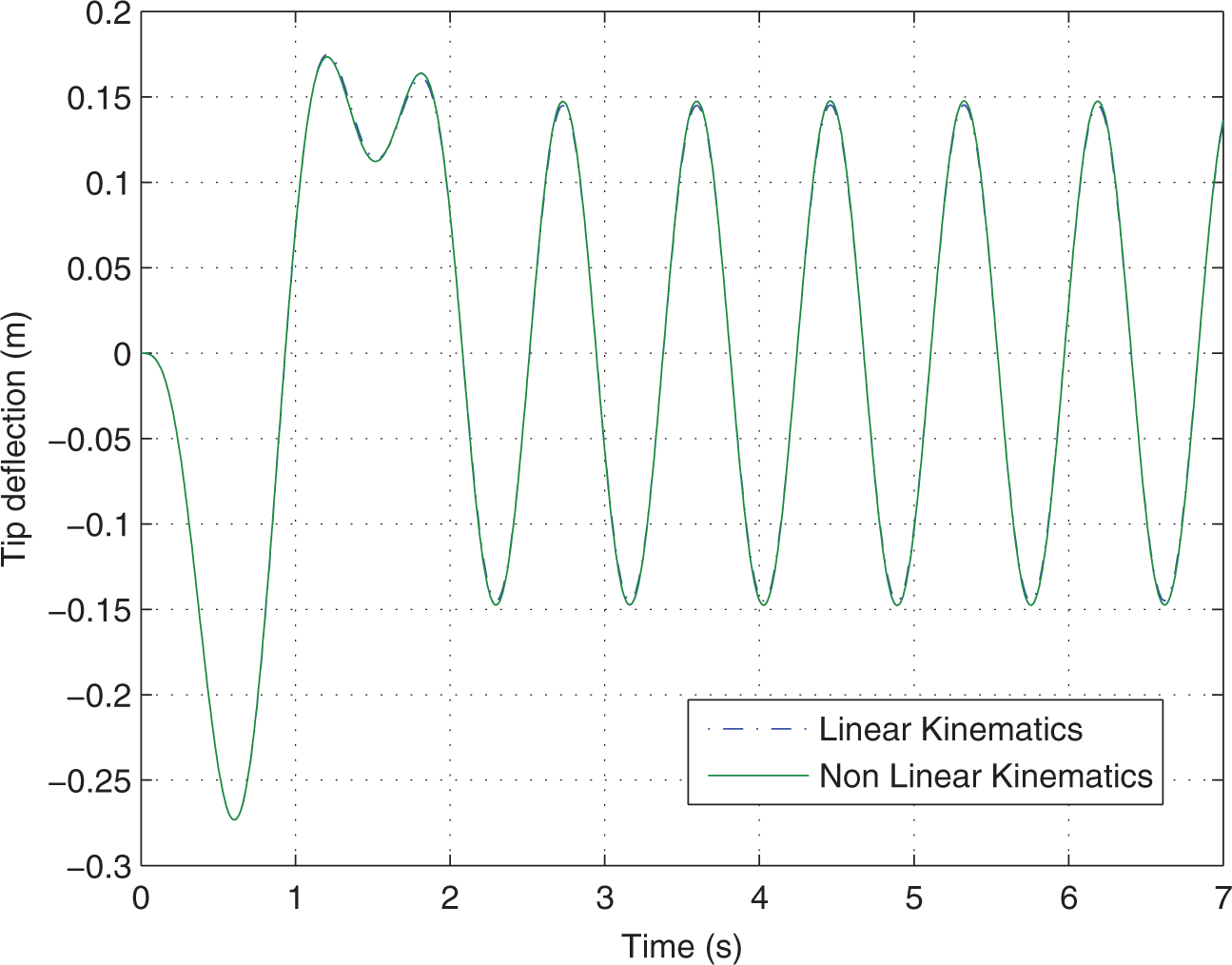
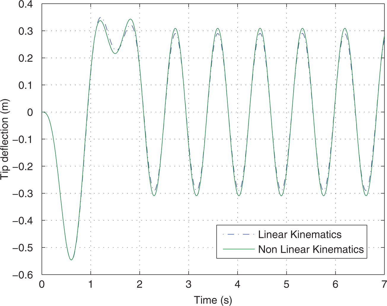
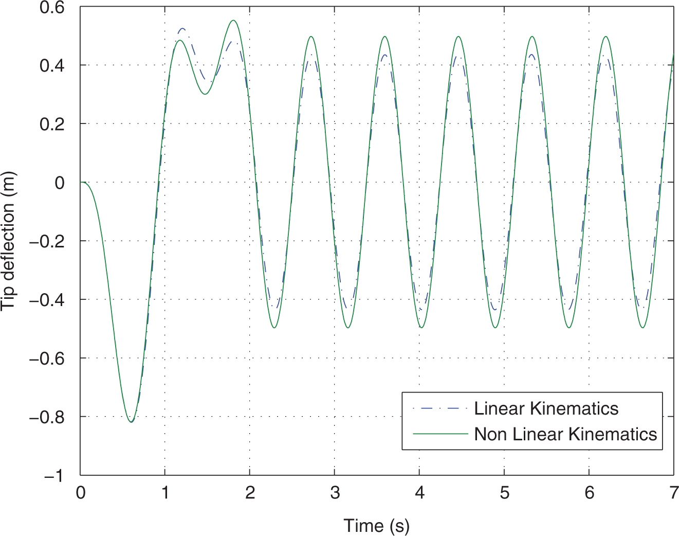

With linear kinematics, the tip deformation is underestimated. These results are similar quantitatively and qualitatively to those shown in Emam (2010). For a one flexible link, the results show that the foreshortening effect is similar to the effect of a nonlinear dynamics when the hub is restrained by a vertical translational and a rotational spring. The number of the flexible modes has little effect on the results. With one flexible mode and A0 = 6 N m, the tip deformation is 12.13% lower with linear kinematics than with a nonlinear kinematics, that is comparable to the 12.40% when two modes where considered. For additional modes, the difference between the responses is insignificant. This shows that the lower modes are dominant.
In addition, to investigate the foreshortening effect on the dynamics when the speed is increasing, a constant torque of 4 N m is applied at the links base. Figures 6 and 7 show the speed and the tip deformation, respectively, for linear and nonlinear kinematics. The results show that with linear kinematics the tip deformation is overestimated. The nonlinear model shows that, for high speed, the deformations are smaller and hence the flexible link is stiffer.
Motion speed, A0 = 4 N m. Tip deflection, A0 = 4 N m.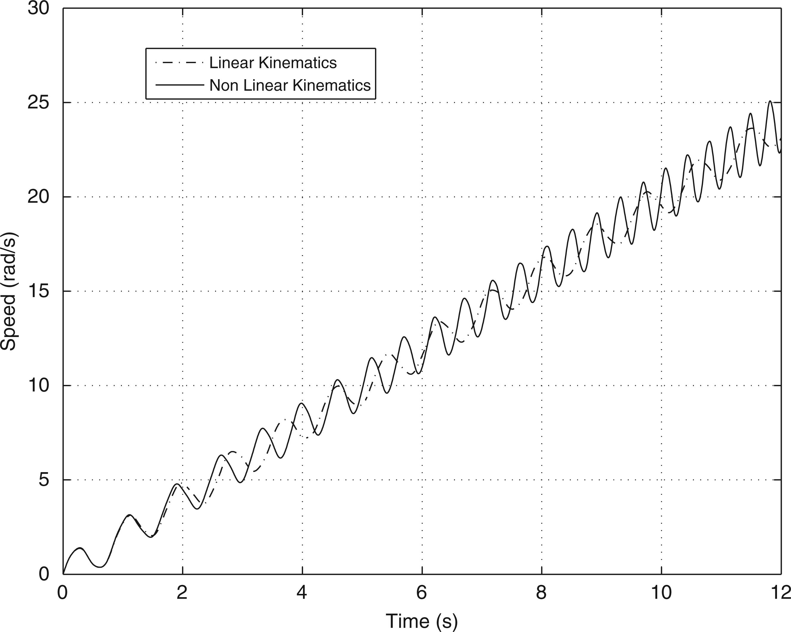
7. Conclusion
In this work, the mathematical model of a flexible link system using Lagrange equations has been presented by taking into account foreshortening effect of the link. This effect was considered using a nonlinear kinematics, that is the elongation of the link along its longitudinal axis. We also showed the effect of the foreshortening on the dynamical response for a sinusoidal torque input at the links hub. The simulations results showed that for small amplitudes the difference between linear and nonlinear kinematics are small. However, for large amplitudes, this difference is more significant and cannot be ignored while controlling flexible links systems.
Footnotes
Funding
This work was supported in part by the NSERC, Canada (grant number 341901-07).