Solving the linear system Ax = b is an active area of research in engineering. Many researchers have applied preconditioners to the linear system Ax = b. In this work, we introduce two new preconditioners for solving linear systems. The best property of the introduced preconditioners is that they can be used under weaker conditions than the previous preconditioners in the literature. We propose preconditioned associated accelerated overrelaxation (AOR) iterative methods with these two new preconditioners, and give the corresponding convergence results. Numerical examples show an improvement in the convergence rate of the AOR preconditioned iterative matrices.
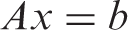
where A ∈ ℛn×n, b ∈ ℛn are given and x ∈ ℛn is unknown. For any splitting, A = M − N with det(M) ≠ 0, the iterative method for solving equation (1) is
For simplicity, without loss of generality, we assume throughout this paper that
where I is the identity matrix, and L and U are strictly lower and upper triangular matrices obtained from A, respectively. The AOR iterative method (Hadjidimos, 1978) is defined as follows
where i = 0, 1, 2,…. Its iteration matrix is
where w and r are real parameters with w ≠ 0.
It is well known that, for certain values of the parameters w and r, we obtain the Jacobi, the Gauss–Seidel and the successive overrelaxation (SOR) methods.
We now transform the original system in equation (1) into the preconditioned form
Then, we can define the basic iterative scheme
where PA = Mp − Np and Mp is nonsingular.
A large number of papers have been written about iterative methods for solving linear systems (Evans and Martins, 1992; Li and Sun, 2000; Evans et al., 2001; Li, 2002; Ding and Chen, 2005a, 2005b, 2006; Li et al., 2007; Wang et al., 2007; Wu et al., 2007; Yun and Kim, 2008; Dehghan and Hajarian, 2010a, 2010b, 2011a, 2011b). Milaszewics (1987) presented the modified Jacobi and Gauss–Seidel iterative methods using the preconditioned matrix where
In Milaszewics (1987) the matrix A has to be an L-matrix with
To date, several kinds of preconditioner P have been presented in which the matrix A has been an L-matrix with equation (6). In many practical problems, the assumption in equation (6) is somewhat too strong. The purpose of this paper is to introduce two new preconditioners under weaker conditions than equation (6).
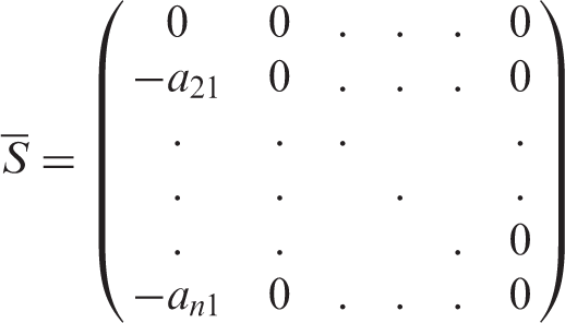
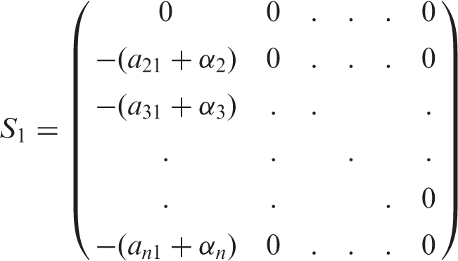
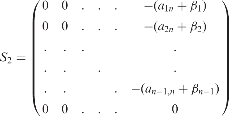
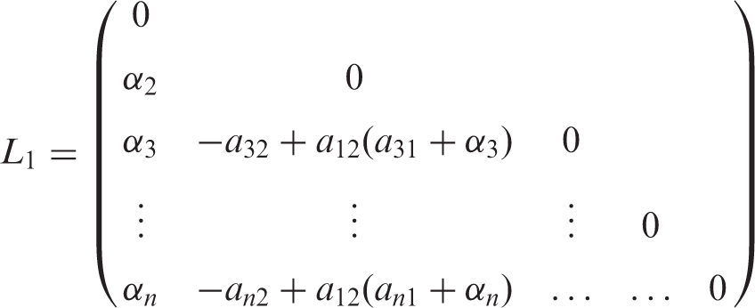
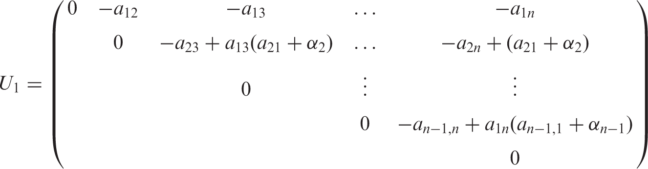
We propose two new preconditioners P1 = I + S1 and P2 = I + S2 where
and αv and βs are real parameters for v = 2, 3, … , n and s = 1, 2, … , n − 1. Assume that
where
and
where
Note that D11, L11 and U11 (D22, L22 and U22) are diagonal, strictly lower and strictly upper triangular parts of S1U = −D11 + L11 + U11(S2A = S2 − S2U − S2L = D22 − L22 − U22), respectively. From P1 and P2, we can obtain
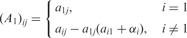
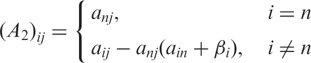
and
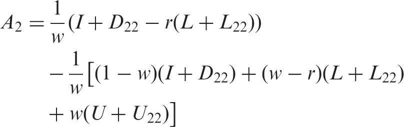
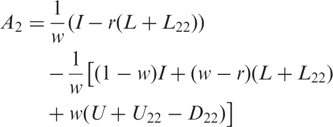
Here we consider the AOR splitting for A1 and A2
and
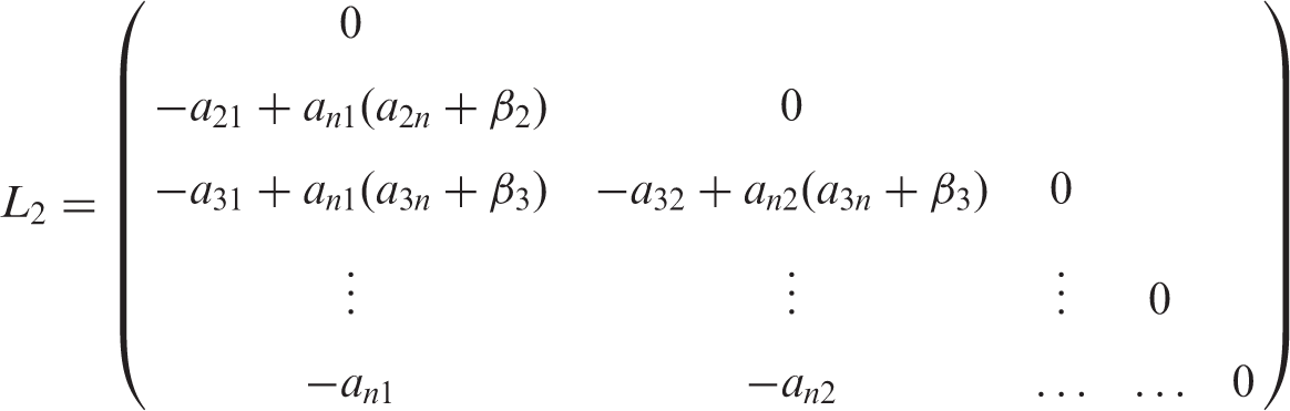
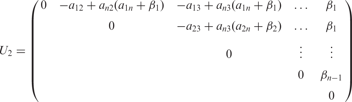
By considering equations (15)–(18), the AOR iteration matrices associated with At are
and
for t = 1, 2, respectively. In the following sections, we will use the above results.
The rest of this paper is outlined as follows: in Section 2, we propose some definitions and lemmas which are essential tools for obtaining our main results. The comparison results are given in Section 3. In Section 4, we employ some numerical examples to support the theoretical results of this paper. In Section 5 we give some concluding remarks to end the paper.
2. Preliminaries
In this section, we give some definitions and lemmas which are essential tools for describing our main results (Berman and Plemmons, 1994; Datta, 1995).
Definition 2.1
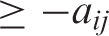
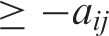
A matrix A is a Z-matrix if aij ≤ 0 for all i, j = 1, 2, … , n such that i ≠ j. Also if aii > 0 i = 1, 2, … , n, the matrix is called an L-matrix. Furthermore, a Z-matrix is a nonsingular M-matrix, if A is nonsingular and A−1 ≥ 0.
Definition 2.2
Let A be a real matrix. The representation A = M − N is called a splitting of A if M is a nonsingular matrix. The splitting is called:
convergent if ρ(M−1N) < 1;
regular if M−1 ≥ 0 and N ≥ 0;
nonnegative if M−1N ≥ 0;
M-splitting if M is a nonsingular M-matrix and N ≥ 0.
Definition 2.3
(Schneider, 1977) An n × n matrix A = (aij) is reducible if we may partition 1, … , n into two nonempty subsets E, F such that aij = 0 if i ∈ E and j ∈ F. If A is not a reducible matrix, we call A is an irreducible matrix.
Lemma 2.1
(Varga, 1981) Let A ≥ 0 be an irreducible matrix. Then
A has a positive real eigenvalue equal to its spectral radius.
If αx ≤ Ax for some nonnegative vector x, x ≠ 0, then α ≤ ρ(A).
If Ax ≤ βx for some positive vector x, then ρ(A) ≤ β. Moreover, if A is irreducible and if 0 ≠ αx ≤ Ax ≤ βx for some nonnegative vector x, then α ≤ ρ(A) ≤ β and x is a positive vector.
Lemma 2.3
(Li and Sun, 2000) Let A = M − N be an M-splitting of A. Then ρ(M−1N) < 1 if and only if A is a nonsingular M-matrix.
Lemma 2.4
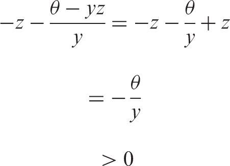
Let θ ∈ (0, 1], y ∈ (−∞, 0), and z ∈ (−∞, 0), then the set Q
is nonempty.
Proof
If we show that , the proof will be complete. We can write
Therefore Q ≠ φ.
Theorem 2.1
Let L(r, w), and (t = 1, 2) be the iteration matrices of the AOR method given by equations (3), (19) and (20) associated with P1and P2, respectively. If A is an irreducible L-matrix with a1vav1 > 0 and ansasn > 0, then for, (v = 2, 3, … , n and s = 1, 2, … , n − 1), 0 < θ ≤ 1 and 0 ≤ r ≤ w ≤ 1 (w ≠ 0) (r ≠ 1), L(r, w), , (t = 1, 2) are nonnegative irreducible matrices.
Proof
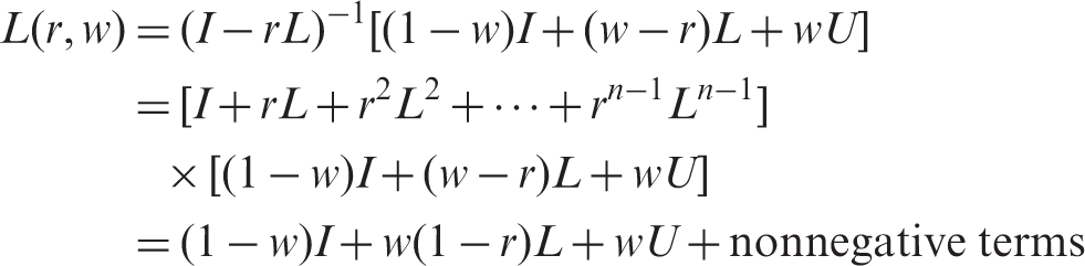
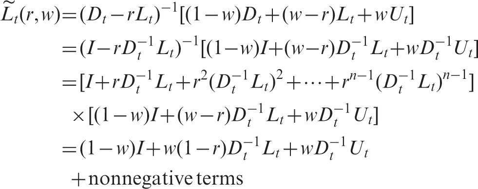
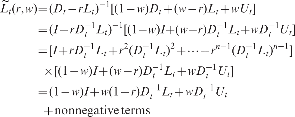
Because A is an irreducible L-matrix, L is a nonnegative strictly lower triangular matrix and U is a nonnegative strictly upper triangular matrix. By equation (3), we have
Since 0 ≤ r ≤ w ≤ 1 (w ≠ 0) (r ≠ 1), we have L(r, w) is nonnegative. We can also get that (1 − w)I + w(1 − r) L + wU is irreducible for irreducible A, hence L(r, w) is also irreducible.
Now, we show that Dt > 0, Lt ≥ 0, Ut ≥ 0, and Dtt ≤ 0. By equations (13) and (14), we can obtain
and
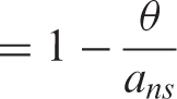
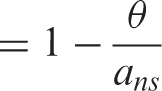
For , (v = 2, 3, … , n and s = 1, 2, … , n − 1), we can write
and
By considering equations (26) and (27), we can get Dt > 0 and Dtt ≤ 0 for t = 1, 2. We can also write
and
Therefore Lt ≥ 0 and Ut ≥ 0 for t = 1, 2. Now from equation (19), we have
By the above results, we can see are nonnegative irreducible matrices for t = 1, 2. Similar to the above proofs, we can show that are nonnegative irreducible matrices for t = 1, 2. The proof is complete. □
Notice that, similar to the proof of the above theorem and using equations (28) and (29), we can conclude that Ltt ≥ 0 for t = 1, 2.
In the next section, applying the above results, we will present the main theorems in this work.
3. Comparison theorems
The spectral radius of the iterative matrix is conclusive for the convergence and stability of the method, and the smaller it is, the faster the method converges when the spectral radius is smaller than 1. In this section, some results for the AOR iterative method with preconditioners P1 and P2 are given.
Theorem 3.1
Let L(r, w), be defined by equations (3) and (19) for t = 1, respectively. If A is an irreducible L-matrix with a1vav1 > 0, then for, (v = 2, 3, … , n), 0 < θ ≤ 1 and 0 ≤ r ≤ w ≤ 1 (w ≠ 0) (r ≠ 1) we have
, if ρ(L(r, w)) < 1
, if ρ(L(r, w)) = 1
, if ρ(L(r, w)) > 1
Proof
Theorem 2.1 implies that L(r, w) is a nonnegative irreducible matrix, hence there exists a positive vector x, such that
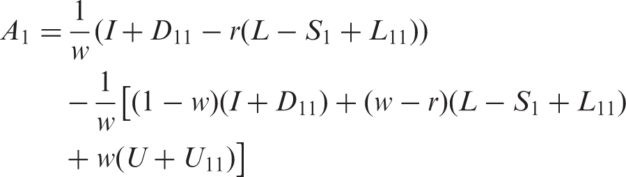
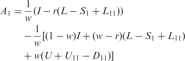
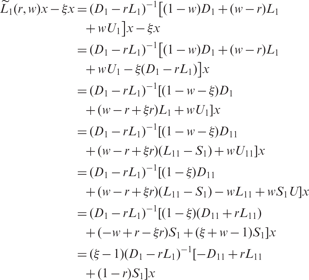
Now using equations (9)–(12), (19) and (32) we can obtain
Now let
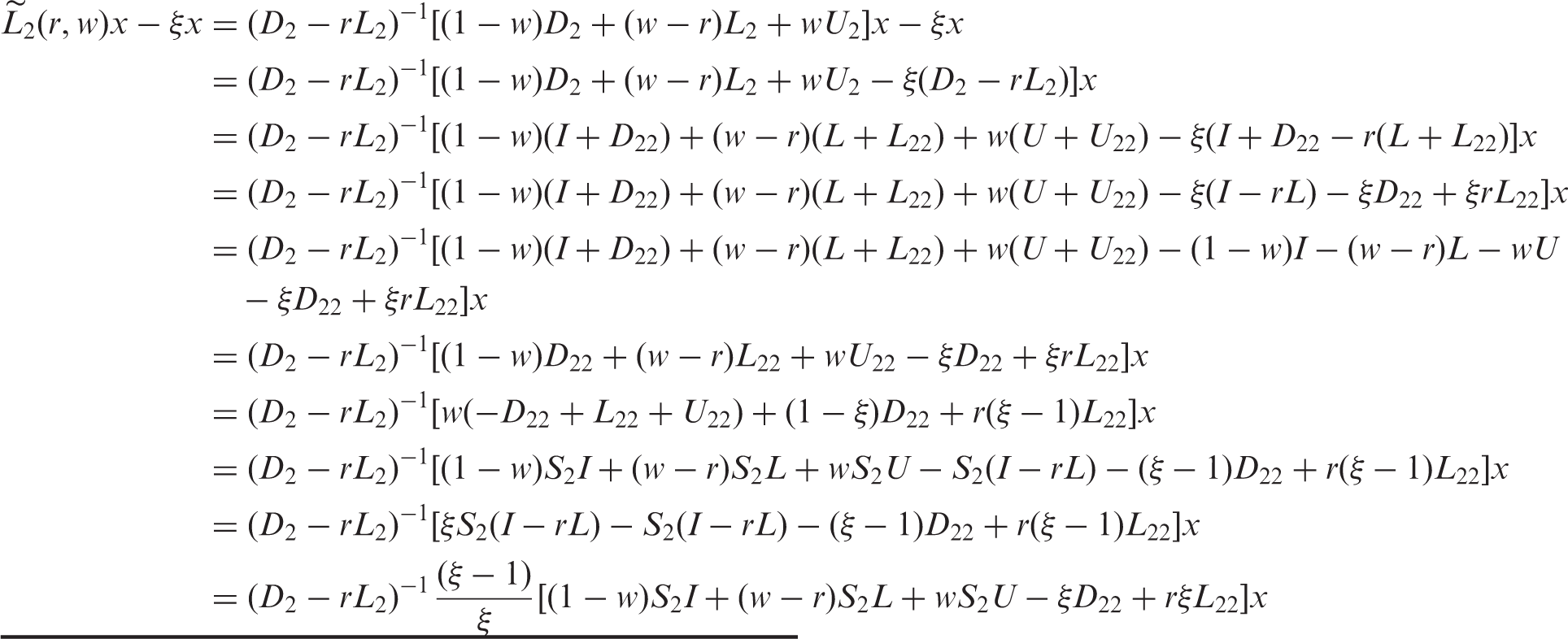
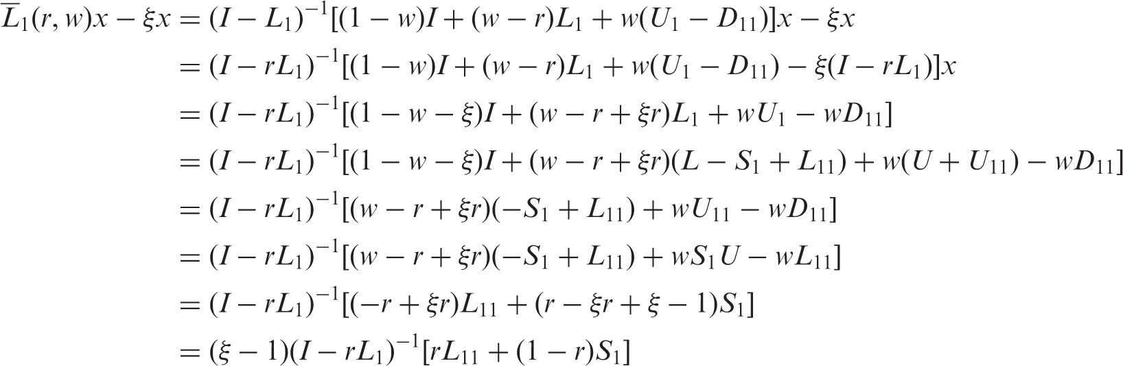
From −D11 ≥ 0, L11 ≥ 0, and S1 ≥ 0, we have [−D11 + rL11 + (1 − r)S1] ≥ 0. Let R = D1 − rL1, we have D1 is a nonsingular M-matrix and rL1 ≥ 0. From Definition 2.2, we have the splitting R = D1 − rL1 as an M-splitting of R. Since is a strictly lower triangular matrix so that . By considering Lemma 2.3, we have R is a nonsingular M-matrix. Therefore (D1 − rL1)−1 ≥ 0, then F ≥ 0.
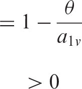
If ξ < 1, then . Therefore . By using Lemma 2.2, we get ;
If ξ = 1, then . Therefore . By using Lemma 2.2, we obtain ;
If ξ > 1, then . Therefore . By using Lemma 2.2, we get .
The proof is complete. □
Theorem 3.2
Let L(r, w), be defined by equations (3) and (19) for t = 2, respectively. If A is an irreducible L-matrix with ansasn > 0, then for (s = 1, 2, … , n − 1), 0 < θ ≤ 1 and 0 ≤ r ≤ w ≤ 1 (w ≠ 0) (r ≠ 1) we have
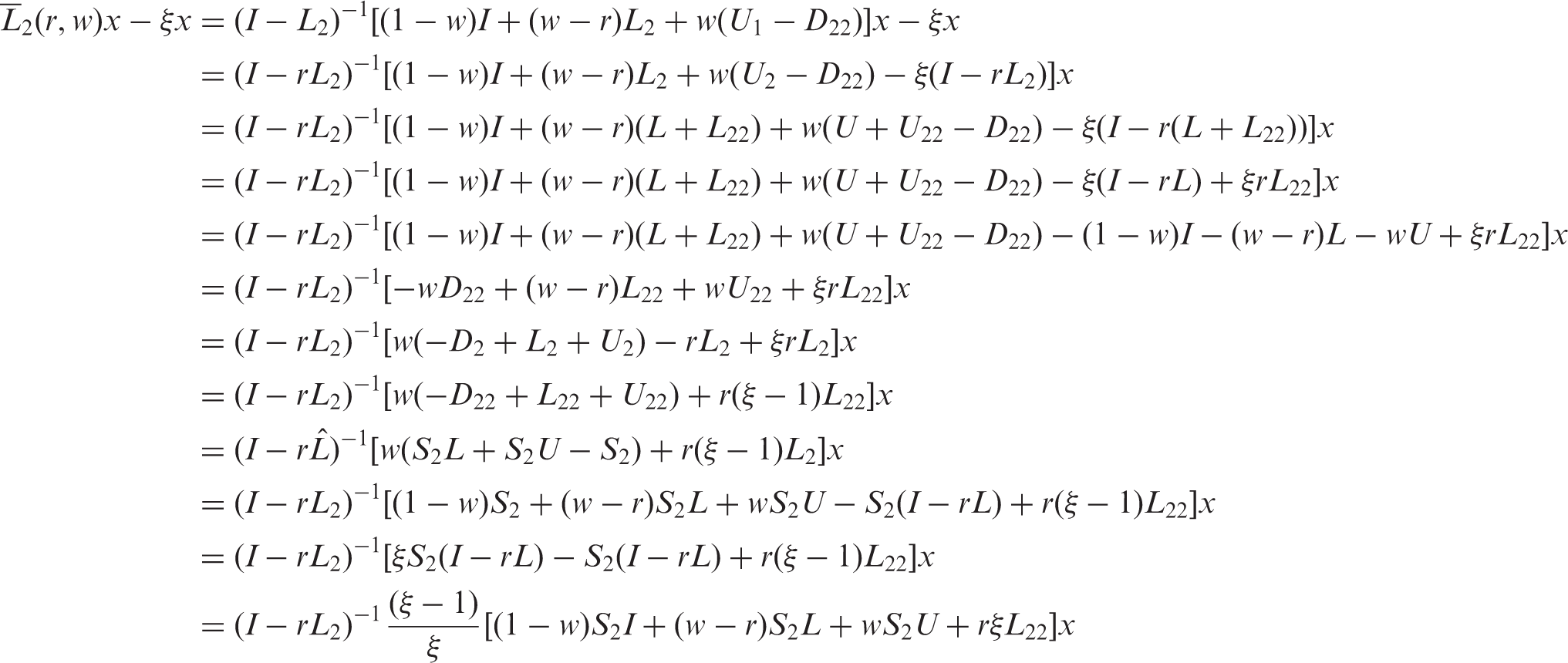
By a similar proof to the previous theorem we can show that H ≥ 0.
If ξ < 1, then . Therefore . By considering Lemma 2.2, we get ;
If ξ = 1, then . Therefore . By considering Lemma 2.2, we obtain ;
If ξ > 1, then . Therefore . By considering Lemma 2.2, we get .
The proof is complete. □
Theorem 3.3
Let L(r, w), be defined by equations (3) and (20) for t = 1, respectively. If A is an irreducible L-matrix with a1vav1 > 0, then for, (v = 2, 3, … , n), 0 < θ ≤ 1 and 0 ≤ r ≤ w ≤ 1 (w ≠ 0) (r ≠ 1) we have
Similar to proof of the previous theorem we can conclude that J ≥ 0.
If ξ < 1, then . Therefore . Using Lemma 2.2 implies that ;
If ξ = 1, then . Therefore . Using Lemma 2.2 implies that ;
If ξ > 1, then . Therefore . Using Lemma 2.2 implies that .
The proof is complete. □
Theorem 3.4
Let L(r, w), be defined by equations (3) and (20) for t = 2, respectively. If A is an irreducible L-matrix with ansasn > 0, then for (s = 1, 2, … , n − 1), 0 < θ ≤ 1 and 0 ≤ r ≤ w ≤ 1 (w ≠ 0) (r ≠ 1) we have
If ξ < 1, then . Therefore . By using Lemma 2.2, we get ;
If ξ = 1, then . Therefore . By using Lemma 2.2, we obtain ;
If ξ > 1, then . Therefore . By using Lemma 2.2, we get .
The proof is complete. □
We know, when w = r the AOR method reduces to the SOR method. For w = r, L(r, w), and (t = 1, 2) are presented by T(w), , and (t = 1, 2) as follows
and
From Theorems 3.1–3.4, we can obtain the following corollaries.
Corollary 3.1
Let T(w), be defined by equations (35) and (36) for t = 1, respectively. If A is an irreducible L-matrix with a1vav1 > 0, then for, (v = 2, 3, … , n), 0 < θ ≤ 1 and 0 < w < 1 we have
, if ρ(T(w)) < 1
, if ρ(T(w)) = 1
, if ρ(T(w)) > 1
Corollary 3.2
Let T(w), be defined by equations (35) and (36) for t = 2, respectively. If A is an irreducible L-matrix with ansasn > 0, then for (s = 1, 2, … , n − 1), 0 < θ ≤ 1 and 0 < w < 1 we have
, if ρ(T(w)) < 1
, if ρ(T(w)) = 1
, if ρ(T(w)) > 1
Corollary 3.3
Let T(w), be defined by equations (35) and (37) for t = 1, respectively. If A is an irreducible L-matrix with a1vav1 > 0, then for, (v = 2, 3, … , n), 0 < θ ≤ 1 and 0 < w < 1 we have
, if ρ(T(w)) < 1
, if ρ(T(w)) = 1
, if ρ(T(w)) > 1
Corollary 3.4
Let T(w), be defined by equations (35) and (37) for t = 2, respectively. If A is an irreducible L-matrix with ansasn > 0, then for (s = 1, 2, … , n − 1), 0 < θ ≤ 1 and 0 < w < 1 we have
, if ρ(T(w)) < 1
, if ρ(T(w)) = 1
, if ρ(T(w)) > 1
In the next section, several numerical examples are given to show the efficiency of the presented preconditioners.
4. Numerical examples
Now let us consider the following examples to illustrate the results obtained in the previous section.
Example 4.1
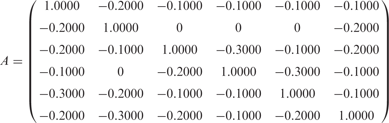
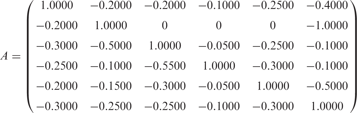
The coefficient matrix A of equation (1) is given by
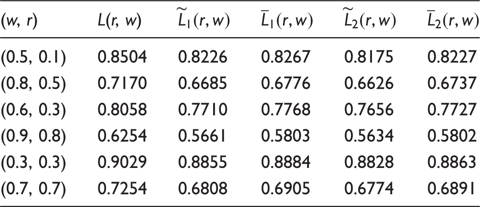
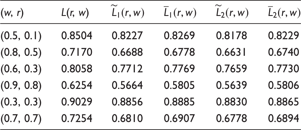
We can see easily, matrix A does not satisfy in equation (6). But we can apply the proposed methods. Tables 1 and 2 display the spectral radii of the corresponding iterative matrices with different parameters w, r, αv, and βs (v = 2, 3, … , 6 and s = 1, 2, … , 5).
The spectral radii of L(r, w), , , , and iterative matrices for θ = 1, αv = 0.0001, and βs = 0.0001 (v = 2, 3,…, 6 and s = 1, 2,…, 5)
(w, r)
L(r, w)
(0.5, 0.1)
0.8504
0.8226
0.8267
0.8175
0.8227
(0.8, 0.5)
0.7170
0.6685
0.6776
0.6626
0.6737
(0.6, 0.3)
0.8058
0.7710
0.7768
0.7656
0.7727
(0.9, 0.8)
0.6254
0.5661
0.5803
0.5634
0.5802
(0.3, 0.3)
0.9029
0.8855
0.8884
0.8828
0.8863
(0.7, 0.7)
0.7254
0.6808
0.6905
0.6774
0.6891
The spectral radii of L(r, w), , , , and iterative matrices for θ = 1, αv = 0.001, and βs = 0.001 (v = 2, 3,…, 6 and s = 1, 2,…, 5)
(w, r)
L(r, w)
(0.5, 0.1)
0.8504
0.8227
0.8269
0.8178
0.8229
(0.8, 0.5)
0.7170
0.6688
0.6778
0.6631
0.6740
(0.6, 0.3)
0.8058
0.7712
0.7769
0.7659
0.7730
(0.9, 0.8)
0.6254
0.5664
0.5805
0.5639
0.5806
(0.3, 0.3)
0.9029
0.8856
0.8885
0.8830
0.8865
(0.7, 0.7)
0.7254
0.6810
0.6907
0.6778
0.6894
Example 4.2
Let
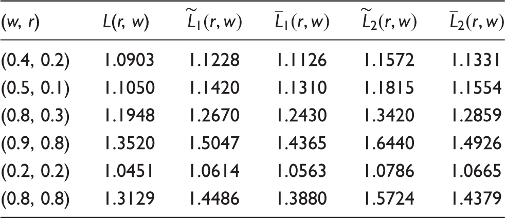
The spectral radii of the corresponding iterative matrices with different parameters w, r, αv, and βs (v = 2, 3, … , 6 and s = 1, 2, … , 5) are shown in Table 3.
The spectral radii of L(r, w), , , , and iterative matrices for θ = 1, αv = 0.0001, and βs = 0.0001 (v = 2, 3,…, 6 and s = 1, 2,…, 5)
(w, r)
L(r, w)
(0.4, 0.2)
1.0903
1.1228
1.1126
1.1572
1.1331
(0.5, 0.1)
1.1050
1.1420
1.1310
1.1815
1.1554
(0.8, 0.3)
1.1948
1.2670
1.2430
1.3420
1.2859
(0.9, 0.8)
1.3520
1.5047
1.4365
1.6440
1.4926
(0.2, 0.2)
1.0451
1.0614
1.0563
1.0786
1.0665
(0.8, 0.8)
1.3129
1.4486
1.3880
1.5724
1.4379
5. Concluding remarks
In this paper, we first proposed two new preconditioners, then applied an AOR iterative scheme to a preconditioned linear system. Second, under mild assumptions, we have introduced a preconditioned AOR method and presented comparison theorems on the preconditioned iterative method for solving linear systems with L-matrices. We have shown that the spectral radius of the proposed methods is smaller than that of the basic AOR method. Numerical examples were also presented to illustrate our results.
Footnotes
Acknowledgements
The authors would like to express their heartfelt thanks to the editor and anonymous referees for their useful comments and constructive suggestions which substantially improved the quality and presentation of this paper.
Funding
This work received no specific grant from any funding agency in the public, commercial, or not-for-profit sectors.
References
1.
BermanAPlemmonsRJ (1994) Nonnegative Matrices in the Mathematical Sciences, Philadelphia: SIAM.
2.
DattaBN (1995) Numerical Linear Algebra and Applications, Pacific Grove: Cole Publishing Co.
3.
DehghanMHajarianM (2010a) The general coupled matrix equations over generalized bisymmetric matrices. Linear Algebra and its Applications432: 15311552.
4.
DehghanMHajarianM (2010b) An efficient algorithm for solving general coupled matrix equations and its application. Mathematical and Computer Modelling51: 11181134.
5.
DehghanMHajarianM (2011a) On the generalized bisymmetric and skew-symmetric solutions of the system of generalized Sylvester matrix equations. Linear and Multilinear Algebra59: 12811309.
6.
DehghanMHajarianM (2011b) Analysis of an iterative algorithm to solve the generalized coupled Sylvester matrix equations. Applied Mathematical Modelling35: 32853300.
7.
DingFChenT (2005a) Iterative least squares solutions of coupled Sylvester matrix equations. Systems & Control Letters54: 95107.
8.
DingFChenT (2005b) Hierarchical least squares identification methods for multivariable systems. IEEE Transactions on Automatic Control50: 397402.
9.
DingFChenT (2006) On iterative solutions of general coupled matrix equations. SIAM Journal on Control and Optimization44: 22692284.
10.
EvansDJMartinsMM (1992) On the convergence of the extrapolated AOR method. International Journal of Computer Mathematics43: 161171.
11.
EvansDJMartinsMMTrigoME (2001) The AOR iterative method for new preconditioned linear systems. Journal of Computational and Applied Mathematics132: 461466.
12.
HadjidimosA (1978) Accelerated overrelaxation method. Mathematics of Computation32: 149157.
13.
LiW (2002) Preconditioned AOR iterative methods for linear systems. International Journal of Computer Mathematics79: 89101.
14.
LiWSunW (2000) Modified Gauss–Seidel type methods and Jacobi type methods forZ-matrices. Linear Algebra and its Applications317: 227240.
15.
LiYTLiCXWuSL (2007) Improvements of preconditioned AOR iterative method forL-matrices. Journal of Computational and Applied Mathematics206: 656665.
16.
MilaszewicsJP (1987) Improving Jacobi and Gauss–Seidel iterations. Linear Algebra and its Applications93: 161170.
17.
SchneiderH (1977) The concepts of irreducibility and full indecomposability of a matrix in the works of Frobenius, König and Markov. Linear Algebra and its Applications18: 139162.
WangXZHuangTZFuYD (2007) Comparison results on preconditioned SOR-type iterative method forZ-matrices linear systems. Journal of Computational and Applied Mathematics206: 726732.
20.
WuMWangLSongY (2007) Preconditioned AOR iterative method for linear systems. Applied Numerical Mathematics57: 672685.
21.
YunJHKimSW (2008) Convergence of the preconditioned AOR method for irreducibleL-matrices. Applied Mathematics and Computation201: 5664.