Control experiments on time-delayed dynamical systems

Abstract

This paper presents simulation and experimental studies of controls for time-delayed dynamical systems. An inverted pendulum made by Quanser is used as a model system. We investigate two control design methods: optimal feedback gain with the semi-discretization method and a high-order control design. Both simulations and experiments are carried out to demonstrate the utility of the control. The semi-discretization method offers optimal controls without increasing the dimensions of the gain vector, while high-order control involves an increased number of gains. The disadvantages and advantages of both methods are discussed with the support of simulation and experimental results. This paper highlights the fact that high-order control is determined by an N^th order filter where N is the discretization level. We have also found that the performance of high-order control appears to be insensitive to N.

Keywords

Dynamical systems time delay stability feedback control

1. Introduction

There is growing interest in the analysis, control and applications of dynamical systems with time delays. Time delay can be part of the system's properties. It can also arise in the control system when there is a signal transport time lag or a delay due to the hardware of the digital controller. The latter is the focus of this paper. In particular, we investigate two control design methods to deal with the time delay in control, and evaluate the performance of the controls designed by these methods with the help of simulations and experiments.

Many engineering applications involve time delay. Space teleoperation and control of unmanned aerial vehicles (UAVs) are notorious for transport delays (Nohmi and Matsumoto, 2002; de Vries, 2005). Singh (1995) has developed a time-delay filter for fuel–time optimal control. Ha and Ly (1996) studied a sampled-data control system with consideration of computational time delay. Time-delayed feedback control was also designed by Fujii et al. (2000) to regulate the librational motion of gravity–gradient satellites in an elliptic orbit. Olgac and his associates have published extensively on the use of delayed resonators for vibration suppression (see Filipovic and Olgac, 1998 for an example). Ali et al. (1998) carried out a study on the stability and performance of feedback controls with multiple time delays by considering the roots of the closed-loop characteristic equation. The of model predictive control also offers a good tool for dealing with time delay (Dumont et al., 1993; Normey-Rico and Camacho, 1999; Rawlings, 2000). Pinto and Goncalves (2002) fully discretized a nonlinear single degree of freedom (SDOF) system to study control problems with time delay. Klein and Ramirez (2001) studied multiple degree of freedom (MDOF) delayed optimal regulator controllers with a hybrid discretization technique where the state equation was partitioned into discrete and continuous portions. Stepan (1998) and Yang and Wu (1998) studied structural systems with time delay. A method using Chebyshev polynomials to approximate general nonlinear functions of time has been developed to handle linear and nonlinear time-delayed periodic systems (Ma et al., 2003, 2005; Deshmukh et al., 2006, 2008; Butcher and Bobrenkov, 2009). This method has also been applied to study optimal control problems.

The stability of delayed dynamical systems has been extensively studied in the literature, and the Lyapunov approach is a popular method (Wu and Mizukami, 1995; Kapila and Haddad, 1999; Gu and Niculescu, 2003). Garg et al. (2007) developed a temporal finite element method to study the stability of time-delayed systems with parametric excitations. Kalmar-Nagy (2005) made use of the piece-wise exact solution of linear differential equations with a single time delay to create a map for stability analysis of the system. Gu and Niculescu (2003) presented an excellent survey of the stability and control of time-delayed systems.

For time-invariant linear systems with time delay, several methods are available for the design of proportional-integral-derivative (PID) controls and their stability analysis. Methods of root locus and Nyquist criterion are quite mature. The Smith predictor is a well-known method (Smith, 1957) that proposes a compensator to stabilize the feedback control designed for the system without time delay. The semi-discretization (SD) method is a well established method in the literature and is used widely in structural and fluid mechanics (Pfeiffer and Marquardt, 1996; Leugering, 2000). This method has been applied to delayed dynamical systems by Insperger and Stepan (2001, 2002), and later extended to study delayed feedback controls (Sheng et al., 2004; Sheng and Sun, 2005). Recently, Insperger and Stepan (2011) published a comprehensive and general overview of the semi-discretization method. The continuous time approximation (CTA) method is an extension of the method of semi-discretization and provides an alternative to handling multiple independent time delays (Sun, 2008; Song and Sun, 2011). Deshmukh et al. (2006) and Butcher and Bobrenkov (2009) have applied Chebyshev collocation to the CTA method. The Chebyshev CTA method provides the most accurate solution of time-delayed dynamical systems.

The remainder of this paper is organized as follows. Section 2 describes the mathematical model of the experimental system made by Quanser. Section 3 discusses the control designs. Section 4 presents the simulation and experimental results of the controls, and compares their performances. Section 5 concludes the paper.

2. The system

The experimental apparatus made by Quanser is shown in Figure 1. It consists of a rotary arm and a rigid rod pendulum. The rotary arm swings horizontally to control the motion of the pendulum. The control objective in this experiment is to stablize the inverted vertical position of the pendulum.

Figure 1.

The inverted pendulum apparatus made by Quanser, Canada.

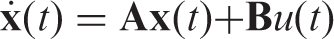
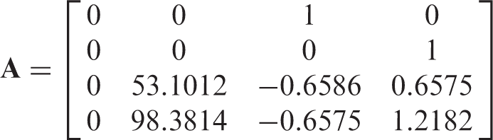
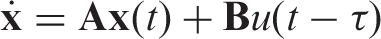
The linearized state equation of the system when the pendulum stands upward can be derived as

\overset{\cdot}{x} (t) = Ax (t) + B u (t)

(1)

where the state vector reads

x (t) = [θ, α, \overset{\cdot}{θ}, \overset{\cdot}{α}] T

, u(t) is the control torque of a DC motor and

A = [001000010 53.1012 - 0.6586 0.6575 0 98.3814 - 0.6575 1.2182]

(2)

B = [0, 0, 274.4012, 273.9627] T

(3)

θ is the angular position of the rotary arm, and α is the angular position of the inverted pendulum. When α = 0, the pendulum stands upward. Two encoders record the angles and the DC motor turns the rotary arm horizontally in order to control the motion of the inverted pendulum.

3. Control designs

3.1. The linear quadratic regulator design

When there is no time delay in the system, linear quadratic regulator (LQR) optimal control of the inverted pendulum with full state feedback u(t) = −Kx(t) can be designed. In this paper, we use the state-weighting matrix Q and the control-weighting factor R given by

Q = diag ([1, 1, 0, 0]), R = 10

(4)

The objective of the optimal control feedback is to minimize both angles θ and α. Its gain is obtained as

K = [k_{1}, k_{2}, k_{3}, k_{4}] = [- 0.31623, 1.9146, - 0.14956, 0.26268]

(5)

This control is provided by Quanser, the maker of the apparatus.

We use this control as the baseline, and digitally introduce time delay to it so that u(t) = −Kx(t − τ) until the closed-loop system becomes unstable. We denote this time delay as τ_max and find τ_max = 0.032 s. We then consider two control design methods that take time delay into account.

3.2. The semi-discretization method design

Now assume that the system has a time delay τ = 0.032 s. We apply the semi-discretization method to design the gain for the control u(t) = −Kx(t − τ) by using the closed-loop system

\overset{\cdot}{x} (t) = Ax (t) - BKx (t - τ)

(6)

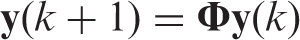
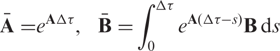
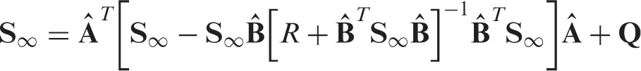
The semi-discretization method leads to a mapping of the extended state vector over the time delay τ

y (k + 1) = Φ y (k)

(7)

where y(k) = [x(k), x(k − 1),…, x(k − N)]_4(1+N)×1 and N is an integer such that Δτ = τ/N is the sample time of the digital control and t = kΔτ. We denote x(t − τ) = x(k − N).

The stability of the control system is determined by the eigenvalues of the mapping Φ, which is a function of the control gain K. Let λ_max = max|λ(Φ)| denote the largest absolute value of eigenvalues of the matrix Φ. Then

| y (k + 1) | \leq λ_{max} | y (k) |

(8)

When λ_max ≤ 1, the system is stable.

If we restrict our interest to a finite and compact region Ω in the gain space of K, we can find the regions of stability and optimal control gains in Ω to minimize λ_max. This leads to the following optimization problem

{min}_{K \in Ω} [λ_{max} (Φ)] subject to λ_{max} \leq 1

(9)

This optimization formulation offers a different approach to the design of feedback controls for linear systems with time delay. The design criterion is to maximize the decay rate of the extended state vector y(k) over one mapping interval. We choose the compact region Ω as

Ω = {(k_{1}, k_{2}, k_{3}, k_{4}) mid - 5 \leq k_{i} \leq 5, i = 1, 2, 3, 4}

(10)

The optimal gain K_opt and the associated optimal λ_max can be found numerically: K_opt = [−0.1598, 1.3981, −0.0959, 0.1943] and λ_max = 0.8426. The optimal λ_max is minimal in Ω. Details of this design method can be found in Elbeyli and Sun (2004), Sheng et al. (2004), and Sheng and Sun (2005).

In region Ω, we have also found a number of gains that are close to K_opt. But, their associated λ_max values are larger than the optimal λ_max. In the vicinity of the optimal gain K_opt, we have experimentally found 11 gains which have better closed-loop control performance for the inverted pendulum than K_opt provides. This difference between the optimal gains determined by the model and by experiments may be attributed to model uncertainties or the optimization criterion of equation (9). Recall that the control objective is to stabilize the upward position α = 0 of the inverted pendulum. The maximized decay rate of the extended state vector y(k) via the mapping Φ may not translate to smaller steady-state oscillations of the angle α around α = 0. Further investigations are certainly needed into this issue. In the results reported later in the paper, we have used the gain K = [−0.1005, 0.9735, −0.0972, 0.2575] with λ_max = 0.9632.

3.3. The high-order control design

Rewrite equation (1) with an explicit time delay τ of the control

\overset{\cdot}{x} = Ax (t) + B u (t - τ)

(11)

Let Δτ = τ/N again be the sample time of the digital control system and t = kΔτ. We denote u(t − τ) = u(k − N). Following the concept of semi-discretization, we construct a mapping from equation (11) as

x (k + 1) = \bar{A} x (k) + \bar{B} u (k - N)

(12)

where

\bar{A} = e A Δ τ, \bar{B} = \int_{0}^{Δ τ} e A (Δ τ - s) B d s

(13)

We have assumed that u(k − N) is constant over a sample interval.

Define an extended state (4 + N) × 1 vector as

y (k) = [x (k), u (k - N), u (k - N + 1), \dots, u (k - 1)] T

(14)

Then, equation (12) can be written in terms of the extended vector without time delay as

y (k + 1) = \overset{\land}{A} y (k) + \overset{\land}{B} u (k)

(15)

where

\overset{\land}{A} = [\bar{A} \bar{B} 0 \dots 0 001 \dots 0 : 0 : 10 \dots \dots \dots 0] \overset{\land}{B} = [0 : : 01]

(16)

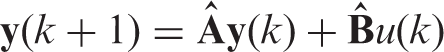
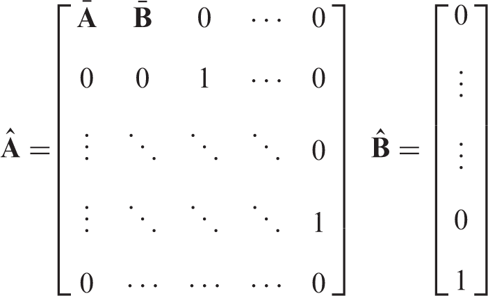
Consider a full extended state feedback control

u (k) = - Ky (k) = - K_{x} x (k) - k_{1} u (k - N) - k_{2} u (k - N + 1) \dots - k_{N} u (k - 1)

(17)

where K = [K_x, k₁,···, k_N] and K_x is 1 × 4. We refer to this control as ‘high-order’ control because the gain matrix K is 1 × (4 + N), as compared to the gain matrix for the LQR optimal control without time delay u(t) = −Kx(t) where K is 1 × 4. We should point out that equation (17) defines an N^th order digital filter for determining the control. Since the dynamics of time-delayed systems exist in an infinite dimensional space, it is quite reasonable to have a high-order filter to determine the control in order to regulate system behavior. The coefficients of the filter offer additional degrees of freedom required to handle the complex dynamics of the system.

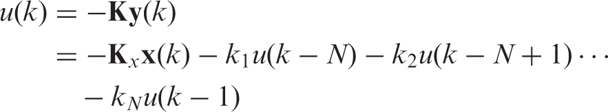
We should also point out that if an integral transformation is introduced to convert the system to one without time delay, as is done in Cai et al. (2003), and the control design is done in the continuous time domain, the filter to determine the control would be in an integration form, which can be discretized leading to the same digital filter as in equation (17).

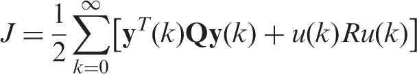
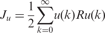
The feedback gain of high-order control can be designed with the digital LQR optimal control formulation to minimize a cost function

J = 12 \sum_{k = 0}^{\infty} [y T (k) Qy (k) + u (k) Ru (k)]

(18)

The optimal gain is given by

K = [R + \overset{\land}{B} T S_{\infty} \overset{\land}{B}] - 1 \overset{\land}{B} T S_{\infty} \overset{\land}{A}

where S_∞ satisfies the algebraic Riccati equation

S_{\infty} = \overset{\land}{A} T [S_{\infty} - S_{\infty} \overset{\land}{B} [R + \overset{\land}{B} T S_{\infty} \overset{\land}{B}] - 1 \overset{\land}{B} T S_{\infty}] \overset{\land}{A} + Q

(19)

For the inverted pendulum, we choose N = 8. Q and R are taken as follows

Q = diag [0.4, 0.01, 0.001, 0.001, 0, \dots, 0] 12 \times 12, R = 1

(20)

The optimal gain is obtained as

K = [- 0.5860, 3.5611, - 0.2689, 0.4904, 0.2352, 0.2215, 0.2085, 0.1961, 0.1842, 0.1728, 0.1619, 0.1515]_{1 \times 12}

(21)

4. Numerical and experimental results

We have carried out extensive numerical simulations and experimental investigations of the inverted pendulum in Figure 1. Figure 2 presents the experimental results of LQR optimal control with the gain in equation (5) without time delay. In the steady state, the angle α oscillates with a peak-to-peak amplitude of 3.1641°. This represents the baseline of the control system.

Figure 2.

The steady-state response of the inverted pendulum system under LQR control without time delay. θ is the angle of the rotary arm and α is the angle of the inverted pendulum. The control objective is to minimize θ and α so as to stabilize the inverted pendulum at α = 0.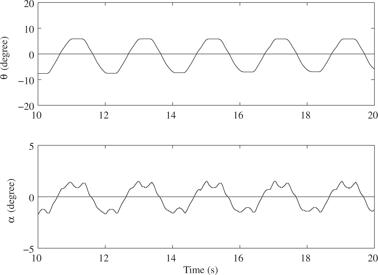

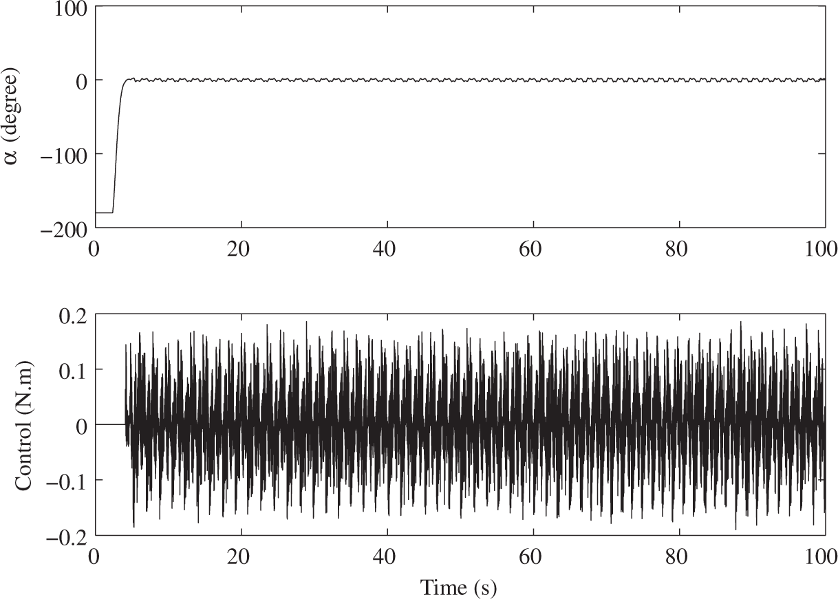
We then gradually and digitally introduce time delay to the control, until the delay reaches 32 ms when the experiment goes unstable as shown in Figure 3. Next, we implement the controls designed with consideration of time delay.

Figure 3.

The unstable response of the inverted pendulum when the LQR control has a time delay of τ = 0.032 s. The LQR control is designed without consideration of time delay. θ is the angle of the rotary arm and α is the angle of the inverted pendulum. The control objective is to minimize θ and α so as to stabilize the inverted pendulum at α = 0.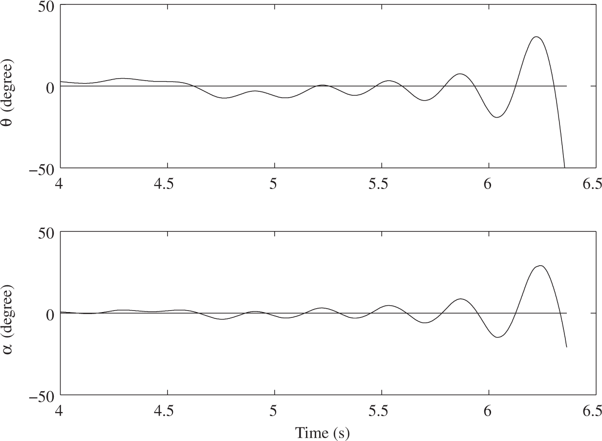

4.1. Control with the semi-discretization method

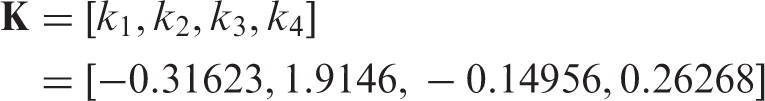
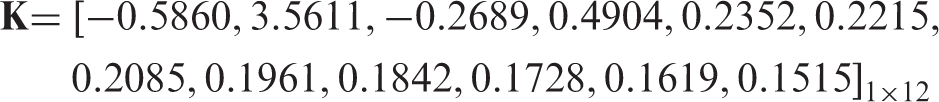
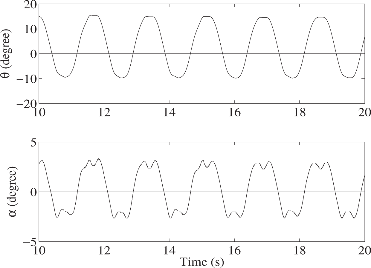
We first implement the control designed with the semi-discretization method and N = 32. The control gain is K = [−0.1005, 0.9735, −0.0972, 0.2575] with λ_max = 0.9632. The simulated control response of the inverted pendulum is shown in Figure 4. Recall that the time delay is 32 ms. Figures 5 and 6 show the transient and steady-state responses of the control experiment. Recall that the control objective is to minimize both θ and α so as to stabilize the upward position of the pendulum at α = 0. In the steady state, the angle α oscillates with a peak-to-peak amplitude of 5.9766° as shown in Figure 6. The system is indeed stabilized in the presence of time delay.

Figure 4.

Simulation of the inverted pendulum under control designed with the semi-discretization method. K = [−0.1005, 0.9735, −0.0972, 0.2575] and λ_max = 0.9632. The top figure shows the response of the system subject to the initial condition α₀ = 5.7296 and θ₀ = 0. Solid line: the angle α of the pendulum. Dash line: the angle θ of the rotary arm. The bottom figure shows the control.

Figure 5.

Experimental transient response of the inverted pendulum under control designed with the semi-discretization method. 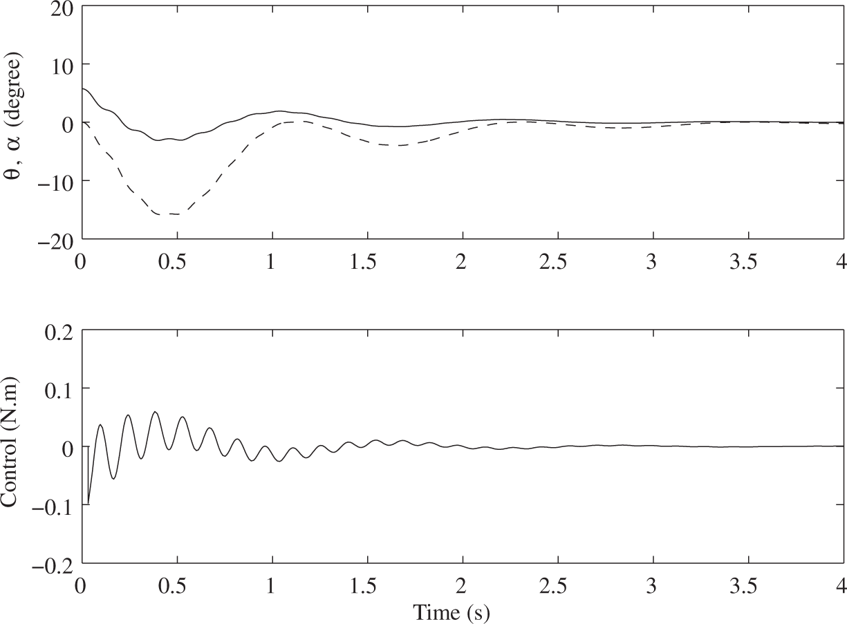K = [−0.1005, 0.9735, −0.0972, 0.2575] and λ_max = 0.9632. The top figure shows the angle α of the pendulum. The bottom figure shows the control.

Figure 6.

The steady-state response of the inverted pendulum under control designed with the semi-discretization method. K = [−0.1005, 0.9735, −0.0972, 0.2575] and λ_max = 0.9632. The top figure shows the angle θ of the rotary arm. The bottom figure shows the angle α of the pendulum. This figure can be compared with Figures 2 and 3.

A note on the initial condition and the transient response of the control experiment is in order. The inverted pendulum controller provided by Quanser includes two parts. The first part destabilizes the downward position and swings the pendulum up. When the pendulum is within about ±5°, the second part starts to stabilize the upward position. At the moment when the stabilizing control starts, the initial conditions for control are random. The control considered in this paper is the second part. Hence, the transient response in Figure 5 does not accurately show the rise time of the control.

4.2. High-order control

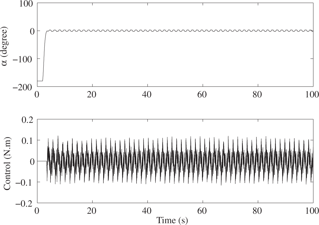
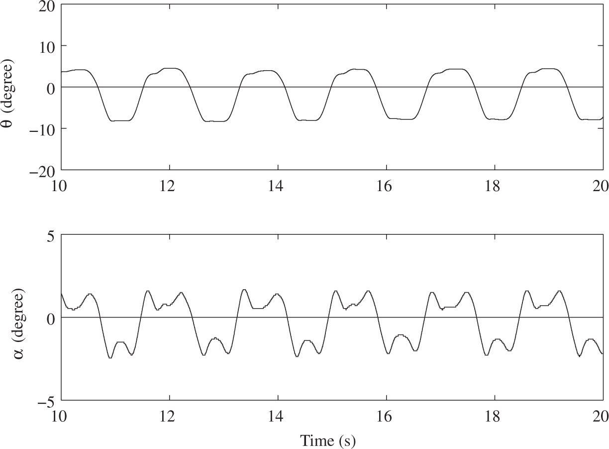
Now, we consider high-order control with N = 8. The control gain is given in equation (21). The simulation is shown in Figure 7. Compared to the results of low-order control by the semi-discretization method in Figure 4, high-order control performs much better. Figures 8 and 9 show the transient and steady-state experimental responses of the inverted pendulum under high-order control. The steady-state oscillations of the angle α have a peak-to-peak amplitude of 4.1309°, smaller than that of low-order control with the semi-discretization method.

Figure 7.

Simulation of high-order control of the inverted pendulum. N = 8. The top figure shows the response of the system from the initial condition α₀ = 5.7296 and θ₀ = 0. Solid line: the angle α. Dash line: the angle position θ of the rotary arm. The bottom figure shows the control.

Figure 8.

Experimental transient response of the inverted pendulum under the high-order control method. N = 8. The top figure shows the response of the angle α. The bottom figure shows the control signal.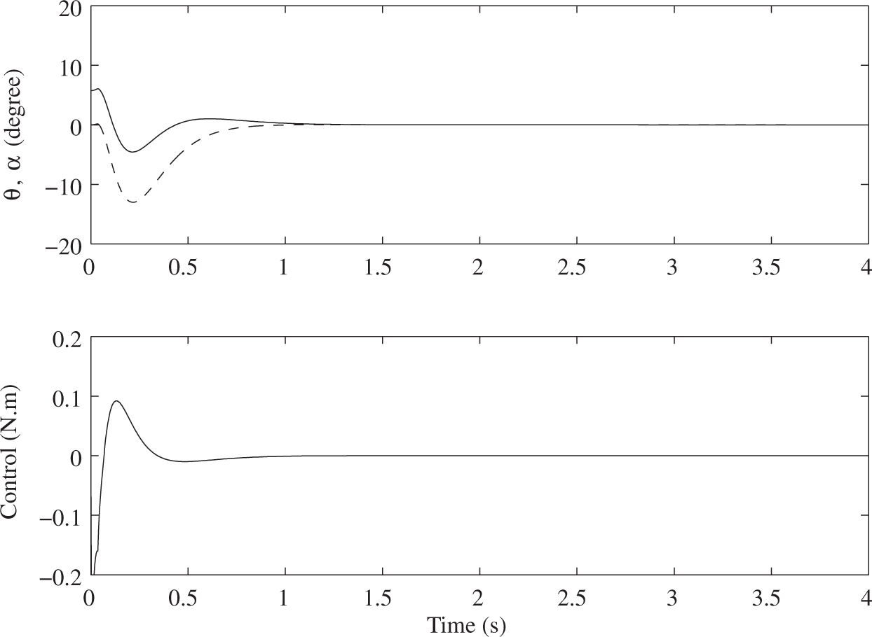

Figure 9.

The steady-state response of the inverted pendulum experiment under high-order control. N = 8. The top figure shows the angle θ of the rotary arm. The bottom figure shows the angle α of the pendulum. This figure can be compared with Figures 2, 3 and 6.

4.2.1. A study of high-order control

In the method of continuous time approximation and semi-discretization, the discretization level N determines how accurate the finite dimensional representation of the time-delayed dynamic system is (Sun, 2008, 2009; Song and Sun, 2011). In the design of high-order control, however, this is no longer the case. This design method leads to a filter of order N to determine the control, as illustrated by the second line in equation (17). This filter is not an approximation of any given system dynamics, but rather a consequence of the full extended state feedback in equation (17). Therefore, we conjecture that the closed-loop dynamics of the control system may be independent of N. In the following, we present simulation and experimental evidence to support this conjecture.

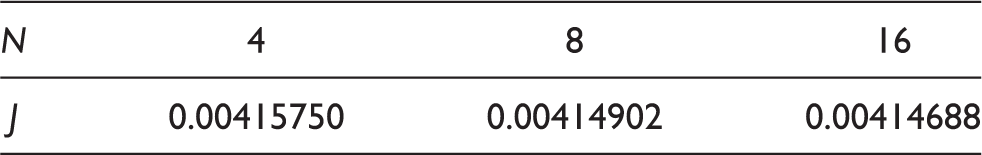
We have selected three values N = 4, 8 and 16 to compare the system responses under high-order control. Numerical simulations of the three cases are shown in Figure 10. The response and control are nearly identical. We have also computed the control performance indices J, listed in Table 1.

Figure 10.

Effect of the discretization level N on the performance of high-order control. The response of the inverted pendulum is simulated. The top figure shows the response α of the system from the initial condition α₀ = 5.7296 and θ₀ = 0 and with N = 4, 8, 16. The bottom figure shows the control. Solid line: N = 4. Dash line: N = 8. Dash–dot line: N = 16. All three lines overlap each other.

Table 1.

The performance indices of three high-order controls with N = 4, 8 and 16. The time integration is over [0, 16]. Note that J from the simulations is much smaller than that from experiments because it is computed over a short time from responses to very small initial conditions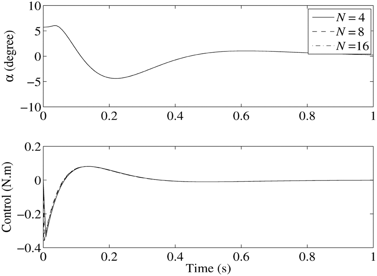

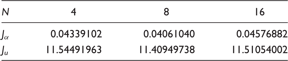
N	4	8	16
J	0.00415750	0.00414902	0.00414688

For all three cases, we have carried out experiments. The difference in the upward positions of the inverted pendulum in the closed-loop system is not noticeable using human eyes. We have collected experimental data and computed the control performance indices to show the differences between the controllers. Since the experiments tend to have rather random initial conditions, we decided to compute the performance index when the system was in a steady state. The results are listed in Table 2. We noticed a difference in the performance indices for different N. This may be attributed to the angle θ.

Table 2.

The performance indices of three high-order controls with N = 4, 8 and 16 in the steady state. The time integration of the experimental data is over [30, 40]

N	4	8	16
J	34.737891	31.648267	32.091666

In the experiments, we noticed that the angle θ of the rotary arm is different in each case. Since θ is used to control the inverted pendulum and is much larger than α, we can define two costs without involving the angle θ as follows

J_{α} = 12 \sum_{k = 0}^{\infty} Q_{22} α 2 (k) + Q_{44} \overset{\cdot}{α} 2 (k)

(22)

J_{u} = 12 \sum_{k = 0}^{\infty} u (k) Ru (k)

(23)

The results are listed in Table 3. It turns out that J_α and J_u are insensitive to N.

Table 3.

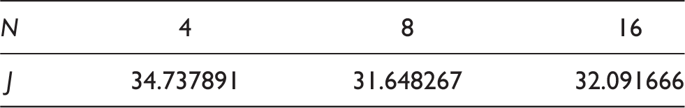
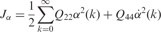
The performance indices J_α and J_u of three high-order controls with N = 4, 8 and 16 in the steady state. The time integration of the experimental data is over [30, 40]

N	4	8	16
J _α	0.04339102	0.04061040	0.04576882
J _u	11.54491963	11.40949738	11.51054002

5. Concluding remarks

In this paper, we have investigated two control design methods: optimal feedback gain with the semi-discretization method and high-order control. Both simulations and experiments were carried out to demonstrate the utility of the control. The semi-discretization method offers optimal controls without increasing the dimensions of the gain vector. This makes the real-time implementation of the control more efficient. However, its performance is not as good as that offered by high-order control. High-order control involves an increased number of gains, and thus has more degrees of freedom to determine the control, which often leads to better performance than a low-order control method such as the one designed with the semi-discretization method. High-order control is determined by an N^th order filter, and becomes history dependent. We have also found that the performance of high-order control appears to be insensitive to the discretization level N.

Footnotes

Funding

This work was supported by the Natural Science Foundation of China (grant number 11172197) and by a key-project grant from the Natural Science Foundation of Tianjin.

References

Ali

Hou

Noori

(1998) Stability and performance of feedback control systems with time delays. Computers and Structures 66(2–3): 241–248.

Butcher

Bobrenkov

(2009) The Chebyshev spectral continuous time approximation for periodic delay differential equations. ASME 2009 international design engineering technical conferences (IDETC) and Computers and Information in Engineering Conference (CIE), San Diego, USA, 30 August – 2 September 2009. New York: ASME.

Cai

G-P

Huang

J-Z

Yang

(2003) An optimal control method for linear systems with time delay. Computers and Structures 81: 1539–1546.

de Vries

(2005) UAVs and control delays, Technical Report TNO-DV3 2005 A054, Netherlands Organization for Applied Scientific Research, Soesterberg, Netherlands.

Deshmukh

Butcher

Bueler

(2008) Dimensional reduction of nonlinear delay differential equations with periodic coefficients using Chebyshev spectral collocation. Nonlinear Dynamics 52(1–2): 137–149.

Deshmukh

Butcher

(2006) Optimal control of parametrically excited linear delay differential systems via Chebyshev polynomials. Optimal Control Applications and Methods 27: 123–136.

Dumont

Elnaggar

Elshafei

(1993) Adaptive predictive control of systems with time-varying time delay. International Journal of Adaptive Control and Signal Processing 7(2): 91–101.

Elbeyli

Sun

(2004) On the semi-discretization method for feedback control design of linear systems with time delay. Journal of Sound and Vibration 273(1–2): 429–440.

Filipovic

Olgac

(1998) Torsional delayed resonator with velocity feedback. IEEE/ASME Transactions on Mechatronics 3(1): 67–72.

10.

Fujii

Ichiki

Suda

Watanabe

(2000) Chaos analysis on librational control of gravity-gradient satellite in elliptic orbit. Journal of Guidance, Control, and Dynamics 23(1): 145–146.

11.

Garg

Mann

Kim

Kurdi

(2007) Stability of a time-delayed system with parametric excitation. Journal of Dynamic Systems, Measurement, and Control 129(2): 125–135.

12.

Niculescu

(2003) Survey on recent results in the stability and control of time-delay systems. Journal of Dynamic Systems, Measurement, and Control 125: 158–165.

13.

U-L

(1996) Sampled-data system with computation time delay: optimal W-synthesis method. Journal of Guidance, Control, and Dynamics 19(3): 584–591.

14.

Insperger

Stepan

(2001) Semi-discretization of delayed dynamical systems. ASME 2001 design engineering technical conferences and computers and information in engineering conference, Pittsburgh, USA, 9–12 September 2001. New York: ASME.

15.

Insperger

Stepan

(2002) Semi-discretization method for delayed systems. International Journal for Numerical Methods in Engineering 55(5): 503–518.

16.

Insperger

Stepan

(2011) Semi-Discretization for Time-Delay Systems, New York: Springer.

17.

Kalmar-Nagy

(2005) A novel method for efficient numerical stability analysis of delay-differential equations. American control conference, Portland, USA, 8–10 June 2005, 2823–2826.

18.

Kapila

Haddad

(1999) Robust stabilization for systems with parametric uncertainty and time delay. Journal of the Franklin Institute 336: 473–480.

19.

Klein

Ramirez

(2001) State controllability and optimal regulator control of time-delayed systems. International Journal of Control 74(3): 281–289.

20.

Leugering

(2000) On the semi-discretization of optimal control problems for networks of elastic strings: global optimality systems and domain decomposition. Journal of Computational and Applied Mathematics 120(1): 133–157.

21.

Butcher

Bueler

(2003) Chebyshev expansion of linear and piecewise linear dynamic systems with time delay and periodic coefficients under control excitations. Journal of Dynamic Systems, Measurement, and Control 125: 236–243.

22.

Deshmukh

Butcher

Averina

(2005) Delayed state feedback and chaos control for time periodic systems via a symbolic approach. Communications in Nonlinear Science and Numerical Simulation 10(5): 479–497.

23.

Nohmi

Matsumoto

(2002) Teleoperation of a truss structure by force command in ETS-VII robotics mission. AIAA Journal 40(2): 334–339.

24.

Normey-Rico

Camacho

(1999) Robustness effects of a prefilter in a Smith predictor-based generalized predictive controller. IEEE Proceedings: Control Theory and Applications 146(2): 179–185.

25.

Pfeiffer

Marquardt

(1996) Symbolic semi-discretization of partial differential equation systems. Mathematics and Computers in Simulation 42(4–6): 617–628.

26.

Pinto

Goncalves

(2002) Control of structures with cubic and quadratic non-linearities with time delay consideration. Journal of the Brazilian Society of Mechanical Sciences 24(2): 99–104.

27.

Rawlings

(2000) Tutorial overview of model predictive control. IEEE Control Systems Magazine 20(3): 38–52.

28.

Sheng

Elbeyli

Sun

(2004) Stability and optimal feedback controls for time-delayed linear periodic systems. AIAA Journal 42(5): 908–911.

29.

Sheng

Sun

(2005) Feedback controls and optimal gain design of delayed periodic linear systems. Journal of Vibration and Control 11(2): 277–294.

30.

Singh

(1995) Fuel/time optimal control of the benchmark problem. Journal of Guidance, Control, and Dynamics 18(6): 1225–1231.

31.

Smith

OJM

(1957) Closer control of loops with dead time. Chemical Engineering Progress 53(5): 217–219.

32.

Song

Sun

(2011) Lowpass filter-based continuous-time approximation of delayed dynamical systems. Journal of Vibration and Control 17(8): 1173–1183.

33.

Stepan

(1998) Delay-differential equation models for machine tool chatter. In: Moon

(ed) Dynamics and Chaos in Manufacturing Processes, New York: Wiley, pp. 165–192.

34.

Sun

(2008) A method of continuous time approximation of delayed dynamical systems. Communications in Nonlinear Science and Numerical Simulation 14(4): 998–1007.

35.

Sun

(2009) Finite dimensional Markov process approximation for stochastic time-delayed dynamical systems. Communications in Nonlinear Science and Numerical Simulation 14(5): 1822–1829.

36.

Mizukami

(1995) Robust stability criteria for dynamical systems including delayed perturbations. IEEE Transactions on Automatic Control 40(3): 487–490.

37.

Yang

(1998) Modal expansion of structural systems with time delays. AIAA Journal 36(12): 2218–2224.