Linear and nonlinear active feedback controls for vortex-induced vibrations of circular cylinders

Abstract

We consider the problem of suppressing oscillations of an elastically mounted rigid cylinder undergoing vortex-induced vibrations by linear and nonlinear active velocity feedback controllers. Each controller relies on an actuator, which imparts an opposing force to the cylinder motion, thereby reducing its high-amplitude oscillations. A strongly coupled fluid–structure numerical model is used to solve the fluid–structure interaction equations. The results show that the choice of the active feedback controller depends on the allowable controlled amplitude of the cylinder. It is found that a cubic velocity feedback controller is more efficient than its linear velocity counterpart when very small controlled amplitudes are desired.

Keywords

Control vortex-induced vibration computational fluid dynamics synchronization circular cylinder

1. Introduction

The flow past freely oscillating cylinders is a canonical problem that has been investigated to understand various flow physics phenomena. When a steady flow passes over a cylinder, with a Reynolds number exceeding 40, an unsteady wake develops. The unsteady wake consists of the well-known von Kármán vortex street. For stationary cylinders, the vortex-shedding frequency f _vs is usually expressed as a nondimensional frequency, called the Strouhal number $(St = f_{vs} D U_{\infty})$ where U _∞ and D are, respectively, the incoming free stream velocity and diameter of the cylinder. The fluid force on the cylinder surface is decomposed into lift and drag components that, respectively, act in the transverse and streamwise directions. The lift component has a zero mean and oscillates at the vortex-shedding frequency. If the cylinder is allowed to flex or rigidly move in the cross-stream direction, this force may cause it to oscillate; a phenomenon that is referred to as vortex-induced vibrations (VIVs). In cases where the vortices are shed at a frequency near the natural frequency of the cylinder, it undergoes high-amplitude oscillations. This phenomenon is called “lock-in” or “synchronization”. These high-amplitude oscillations can impede the function of the cylinder or result in fatigue and degradation of the structural components holding the cylinder. For a comprehensive review of the VIV and the associated synchronization phenomenon of cylinders, the reader is referred to Bearman (1984), Williamson and Roshko (1988), Williamson (1996), Williamson and Govardhan (2004), Jauvtis and Williamson (2004), and Gabbai and Benaroya (2005).

Reduction of the high oscillation amplitudes that are induced by VIVs is desired for enhancing the structures' safety and increasing their lifetime. This can be achieved by reducing the strength of the generated vortices and/or controlling the motion of the cylinder in an appropriate manner. Active (Gad-el-Hak, 2000; Choi et al., 2008) and passive control (Zdravkovich, 1981; Walshe and Wootton, 1979) mechanisms of VIVs have been explored, both experimentally and numerically. Some of the proposed passive controllers include wire ropes and impact, tuned, and structural dampers (Walshe and Wootton, 1979). The wire ropes cause an increase in the natural frequency and damping of the structure. Impact and tuned dampers absorb a considerable amount of energy from the vibrating structure. However, these dampers may not be effective over a wide range of oscillation amplitudes and may be constrained to a limited frequency range (Walshe and Wootton, 1979; Baz and Ro, 1991).

Active flow control mechanisms, such as suboptimal flow blowing and suction (Akhtar and Nayfeh, 2008) or acoustic feedback (Blevins, 1985; Ffowcs Williams and Zhao, 1988; Huang, 1996), have also been proposed to control VIVs. Akhtar and Nayfeh (2008) observed a suppression of the fluctuating forces and obtained more than 40 % reduction in the mean drag coefficient using a couple of suction actuators on a stationary cylinder. Blevins (1985) experimentally observed that sound waves can affect vortex shedding. In particular, the introduction of sound waves with frequencies close to the natural vortex-shedding frequency can alter the shedding frequency and force it to follow the imposed sound frequency. Ffowcs Williams and Zhao (1988) used sound as an active controller to alter the shedding process. The control loop processed signals from hot-wires placed in the cylinder wake and fed them back to the flow using a loudspeaker in a way that affects the shedding process. They observed a reduction in the velocity fluctuations by more than 30 dB. They also observed that the phase of the control signal is an important factor in suppressing the VIVs because a phase reversal of the signal could further amplify the oscillation amplitudes. Huang (1996) locally introduced sound waves into the flow to influence the shear layer on one side of the cylinder. Suppression of the vortex shedding was observed by the destructive interference of the two shear layers.

The control mechanisms discussed above aim at suppressing or delaying the vortex-shedding mechanisms. Another approach for VIV suppression is to directly control the cylinder motion using active feedback controllers. These controllers make use of an actuator signal, which imparts an opposing force to the cylinder motion, thereby reducing the cylinder high-amplitude oscillations. Baz and Ro (1991) implemented a velocity feedback controller to dampen VIVs of a circular cylinder. They used a permanent magnetic d.c. linear actuator and a stator. The actuator was placed inside the cylinder and the stator was anchored to the wall of the wind tunnel. An accelerometer was used to measure the cylinder acceleration. The signal from this accelerometer was integrated to yield the cylinder velocity. This signal was amplified and used to drive the actuator in such a way to impart a force that opposes the oscillation velocity of the cylinder. They were able to obtain more than an 80% reduction in the amplitude of the oscillations in the synchronization regime. Govardhan and Williamson (2006) implemented a mechanical damper that takes the velocity of the cylinder and feeds it, after amplification, to the cylinder through a spring in such a way that it imparts a force in phase with the cylinder velocity. Their results show that the peak amplitude of the vibration is significantly affected by the mass-damping parameter (α), which is directly proportional to the damping ratio.

In this work, we consider the option of using active linear and nonlinear velocity feedback controllers to suppress VIVs. To assess their effectiveness, we compare their performance and required power levels to suppress the motion of the cylinder. In particular, we aim to determine the most effective control law that requires minimum power to achieve any desired controlled amplitude. The focus is on the synchronization region where the oscillation amplitudes are relatively high. The lift on the cylinder can be modeled or determined from phenomenological models (Skop and Griffin, 1973; Nayfeh et al., 2003; Abdelkefi et al., 2012) or numerical simulations of the flow field. In this work, the second option is used. The approach is then to consider, the fluid flow, the cylinder motion, and the controls as a single dynamical system. A strongly coupled fluid–structure-control numerical model is then used to determine the cylinder response to the flow and controls.

The rest of this paper is organized as follows. In Section 2, we discuss the fluid flow solver, modeling of the cylinder with control laws, and validation of the coupling scheme used to solve the fluid and cylinder interaction problem. In Section 3, we compare the responses of the cylinder obtained with both controllers for a range of Reynolds number. In Section 4, we evaluate the performances of the two controllers based on the required power and optimize their configurations. Conclusions are presented in Section 5.

2. Mathematical modeling and numerical simulations

2.1. Fluid flow solver

The numerical solution of the equations governing the interaction of a flow with a cylinder that is free to oscillate is very challenging. The challenge arises because the boundary conditions change as the cylinder moves. Different formulations have been proposed and developed for simulating the flow over oscillating structures or bodies. These formulations include the immersed boundary (IB) (Mittal and Iaccarino, 2005), arbitrary Lagrangian–Eulerian (ALE) (Hirt et al., 1974), and accelerated reference frame (ARF) (Blackburn and Henderson, 1999) methods. In this work, we use a parallel computational fluid dynamics (CFD) code (Akhtar, 2008; Akhtar et al., 2009a), in which the incompressible continuity and unsteady Navier–Stokes equations are solved using an ARF technique. In this technique, the momentum equation is directly coupled with the cylinder motion by adding a reference frame acceleration term (Blackburn and Henderson, 1999; Akhtar, 2008); the outer boundary conditions of the flow domain are then updated using the response of the cylinder. The governing equations can be represented as follows:

\partial u_{j} \partial x_{j} = 0

(1)

\partial u_{i} \partial t + \partial \partial x_{j} (u_{j} u_{i}) = - \partial p ρ \partial x_{i} + ν \partial 2 u_{i} \partial x_{j} \partial x_{j} - \overset{\cdot\cdot}{x_{i}}

(2)

where i, j = 1, 2, 3, u _i represent the Cartesian velocity components (u, v, w), ρ represents the fluid density, and p and ν are the pressure and kinematic viscosity of the fluid, respectively. Here,

{\overset{··}{x}}_{i} = a

is used to denote the cylinder acceleration in the cross-flow direction for the case considered. In the implemented flow solver, the governing equations are nondimensionalized using the cylinder diameter D as a reference length and the incoming free-stream velocity U _∞ as a reference velocity. The Reynolds number is defined as

Re = U_{\infty} D ν

At the domain boundary, the velocity boundary condition is modified to include the effect of the moving cylinder; that is,

u = u_{D} - v

(3)

where u _D is the velocity in the inertial frame of reference and

v = \overset{\cdot}{x}

is the cylinder velocity. On the cylinder surface, the velocity boundary condition is u _i = 0. The pressure boundary condition is obtained by dotting the domain unit outward normal n with equation (2) and using the vector identity ∇² u = ∇(∇.u − ∇ × ∇ × u). The result is

\partial p \partial n = ρ n \cdot [(u \cdot \nabla) u - ν \nabla \times \nabla \times u - \overset{··}{x} - \partial u \partial t]

(4)

On the far field boundary,

\partial u_{i} / \partial t = - {\overset{··}{x}}_{i}

, whereas on the cylinder surface ∂u _i/∂t = 0.

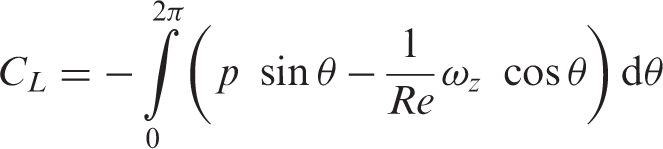
The lift coefficient is computed from the surface pressure as

C_{L} = - \int_{0}^{2 π} (p \sin θ - 1 Re ω_{z} \cos θ) d θ

(5)

where ω_z is the spanwise vorticity component on the cylinder surface and θ is the angle that the outer normal of the area component makes with the flow direction. As shown in Figure 1, a body conformal “O”-type grid is employed to simulate the flow over the cylinder. We employ curvilinear coordinates (ξ, η, ζ) in an Eulerian reference frame. For the specific case of a circular cylinder, the generalized coordinates (ξ, η, ζ) can be represented by polar coordinates (r, θ, z). Details of the numerical discretization and the parallel implementation can be found in Akhtar (2008) and Akhtar et al. (2009a,b).

Figure 1.

A two-dimensional layout of an “O”-type grid in the (r, θ)-plane.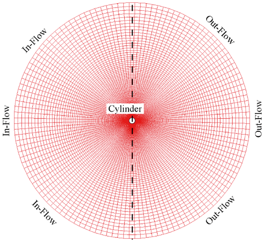

2.2. Representation of the active feedback controllers

The linear controller imparts a force that is proportional to the velocity of the cylinder. The governing equation of an elastically mounted rigid circular cylinder subjected to external fluid forces as shown in Figure 2 with an active linear controller is then expressed as

M \overset{··}{Y} + C \overset{\cdot}{Y} + K Y = F_{Y} (t) - K_{c} \overset{\cdot}{Y}

(6)

where M is the mass of the cylinder per unit length, C and K are the structural damping and stiffness, respectively, F _Y(t) characterizes the time-dependent external force exerted by the fluid flow on the cylinder, and

K_{c} \overset{\cdot}{Y}

is the linear control force with K _c being a positive constant.

Figure 2.

A schematic diagram of an elastically mounted cylinder.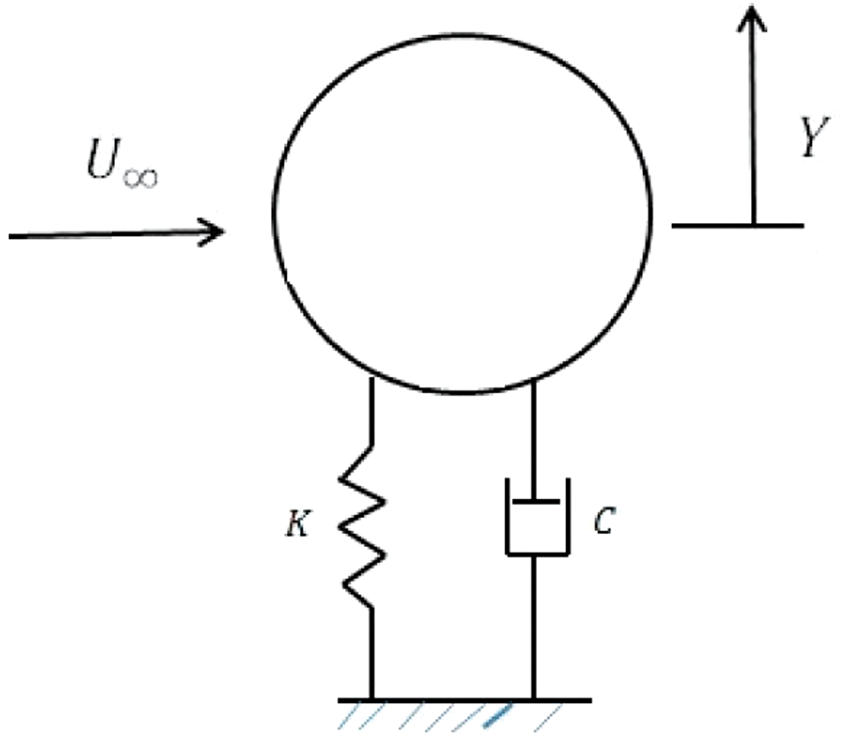

Using the diameter of the cylinder D and the incoming free-stream velocity U _∞ as length and velocity scales, respectively, we rewrite equation (6) in nondimensional form as

\overset{··}{Y} * + (β U_{r}) \overset{\cdot}{Y} * + (2 π U_{r}) 2 Y * = 2 π m * C_{L}

(7)

where Y* = Y/D is the nondimensional transverse cylinder displacement, U _r = U _∞/f _n D is the reduced velocity, β = (4πζ + K _c/M f _n) is the controlled damping term, f _n is the natural frequency of the cylinder,

ζ = C / C_{crit} = C / 2 \sqrt{KM}

is the structural damping ratio, m* = M/M _f is the mass ratio, and

M_{f} = 14 π ρ D 2

represents the fluid mass per unit length replaced by the cylinder. Equation (7) can be equivalently written as a system of two coupled first-order ordinary differential equations; that is,

\overset{\cdot}{y_{1}} = y_{2},

(8)

\overset{\cdot}{y_{2}} = - (2 π U_{r}) 2 y_{1} - β U_{r} y_{2} + 2 π m * C_{L},

(9)

where y ₁ = Y* and

y_{2} = \overset{\cdot}{Y} *

The nonlinear controller imparts a force proportional to the cubic velocity of the cylinder. The governing equation of an elastically mounted rigid circular cylinder subjected to external fluid forces with a cubic velocity feedback controller is then expressed as

M \overset{··}{Y} + C \overset{\cdot}{Y} + K Y = F_{Y} (t) - G \overset{\cdot}{Y} 3,

(10)

where

G \overset{\cdot}{Y} 3

is the nonlinear control law and G is a positive constant. In nondimensional form, equation (10) is written as

\overset{··}{Y} * + (4 π ζ U_{r}) \overset{\cdot}{Y} * + (2 π U_{r}) 2 Y * + γ U_{r} \overset{\cdot}{Y} * 3 = 2 π m * C_{L},

(11)

where γ = G/(M/f _n D ²). Equation (11) can be equivalently written as a system of two coupled first-order ordinary differential equations as

\overset{\cdot}{y_{1}} = y_{2},

(12)

\overset{\cdot}{y_{2}} = - (2 π U_{r}) 2 y_{1} - 4 π ζ U_{r} y_{2} - α U_{r} y_{2}^{3} + 2 π m * C_{L} .

(13)

2.3. Coupling scheme and validation

In performing the simulations, equations (1) and (2), which govern the dynamics of the fluid flow, and equations (7) or (11), which govern the dynamics of the cylinder, must be solved in a coupled manner. The motion of the cylinder requires values of the fluid loads. On the other hand, determining the fluid loads requires knowledge of the motion of the cylinder. An efficient approach to account for this coupling is the Hamming fourth-order predictor–corrector technique (Carnahan et al., 1969). This method enables simultaneous integration of the governing equations of the fluid and cylinder. The basic idea of this technique is to first predict the cylinder motion (displacement, velocity, and acceleration) and plug it in the CFD code to compute the fluid loads. These loads are then used to compute the new states of the cylinder based on a corrector scheme. These steps are repeated until a match between the fluid loads and the cylinder position, that is defined by a specified conditional error at each time step, is reached.

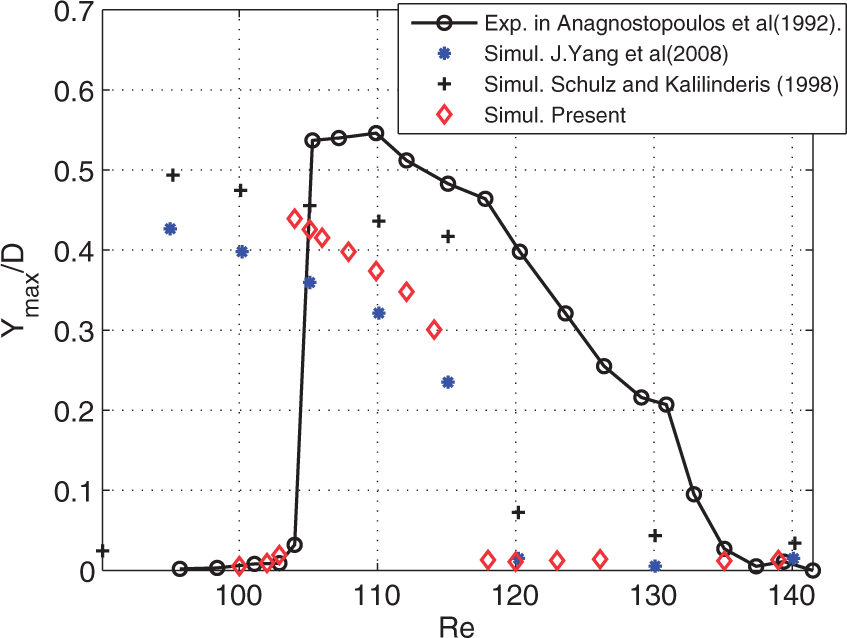
We validate the current simulation scheme by comparing its results with experimental results (Anagnostopoulos and Bearman, 1992) and other numerical simulations (Schulz and Kallinderis, 1998; Yang et al., 2008). We note that, for validation purposes, we perform numerical simulations without the control laws, using the same parameters (m* = 149.10 and ζ = 0.0012) as in the experimental work (Anagnostopoulos and Bearman, 1992). We employ 192 × 256 grid points in the r− and θ− directions, respectively, with a computational domain of 25D. We increase the Reynolds number with small increments in the range 95 ≤ Re ≤ 140. This range corresponds to reduced velocities in the range 5.29 ≤ U _r ≤ 7.79.

A comparison of the variation of the maximum amplitude, Y _max/D, of the cylinder oscillations with the Reynolds number Re as obtained in our simulation and previous experimental (Anagnostopoulos and Bearman, 1992) and numerical simulations (Schulz and Kallinderis, 1998; Yang et al., 2008) is presented in Figure 3. Inspecting this figure, we note that we are able to obtain a better agreement of the location of the bifurcation point (onset of synchronization) with the experimental results than previously reported numerical simulations (Schulz and Kallinderis, 1998; Yang et al., 2008). Still, there is a small difference between our simulations and the experimental data (Anagnostopoulos and Bearman, 1992) when comparing the maximum amplitude and the range of the synchronization regime. This difference, which has been reported by the other numerical studies (Yang et al., 2008; Schulz and Kallinderis, 1998), could be due to the three-dimensional effects, since the experiments were performed without end plates.

Figure 3.

Comparison of maximum displacement amplitudes as predicted in present computations (⋄) with the experimental measurements of Anagnostopoulos and Bearman (1992) (-○) and numerical computations of Yang et al. (2008) (*) and Schulz and Kallinderis (1998) (+).

3. Results and discussion

To investigate the performance of the linear and nonlinear active controllers, we performed numerical simulations of the flow in the range 95 ≤ Re ≤ 125, which corresponds to reduced velocities in the range 5.29 ≤ U _r ≤ 6.96. We considered a mass ratio m* = 149.10 and a damping ratio ζ = 0.0012. In the performed simulations, the flow developed from rest and the cylinder motion was allowed to start after 1000 time steps, which provided a sufficient time for the steady-state response to be achieved. This response, generated for each of the considered Reynolds numbers, was used as the initial condition at which the controller was implemented. After reaching steady state, the data was collected and the frequencies f _vs and f _co of vortex shedding and cylinder oscillations were determined.

Variations of the root mean square (rms) oscillation amplitudes of the cylinder with the Reynolds number are presented in Figure 4(a) and (b) for the linear and cubic velocity feedback controls, respectively, using different control gains. We first consider the response of the uncontrolled cylinder (i.e. K _c = 0 and G = 0) marked in Figure 4(a) and (b) by the dashed lines. Below Re = 104, the oscillation amplitude remains very low. A significant increase in the amplitude is noted near Re = 104. Under this flow condition, the vortices are shed at a frequency close to the cylinder natural frequency, deviating slightly from the shedding frequency of the stationary cylinder. This phenomenon is referred to as “synchronization” and Re = 104 is defined as the Reynolds number corresponding to the onset of the VIVs. The synchronization regime extends to Re = 114. Above this Reynolds number, the oscillation amplitude drops to very small values.

Figure 4.

Variation of the cylinder displacement (Y _rms/D) with the Reynolds number using (a) linear velocity and (b) cubic velocity feedback controllers for different gain values.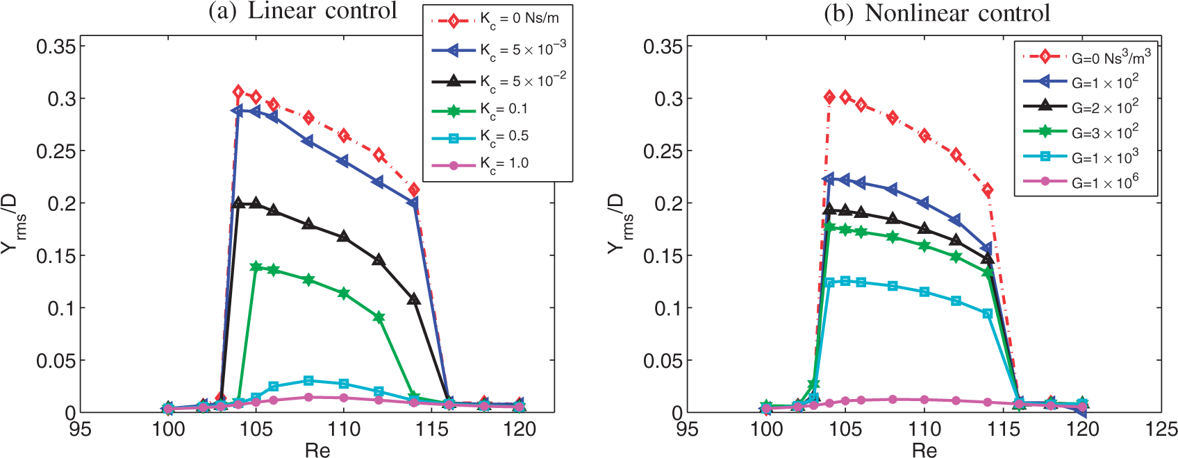

Next, we consider the response of the cylinder when implementing the feedback controllers (i.e. K _c ≠ 0 and G ≠ 0) over the same range of Reynolds number. We consider different values of the linear and nonlinear gains K _c and G. Comparing the responses of the uncontrolled (dashed line) and controlled motions (solid lines), we conclude from Figure 4(a) and (b) that both feedback velocity controllers can be used to reduce the oscillation amplitudes of the cylinder. This effect is evident throughout the synchronization regime.

Figure 4(a) illustrates the effect of increasing the linear control gain on the cylinder oscillations. The results show that, when Re = 105, an amplitude reduction of 4.5% is obtained when K _c = 5 × 10⁻³ Ns/m. Reductions of 54% and 95% are obtained when K _c = 0.1Ns/m and 1.0Ns/m, respectively. It is interesting, however, to note that the onset of synchronization is delayed and the extent of synchronization is reduced when higher gains are used. A similar qualitative behavior was observed by Govardhan and Williamson (2006). They observed a collapse of the peak response amplitude for various values of the combined mass-damping parameter (α = m ^*ζ). It is interesting to note from figure 8(b) of Govardhan and Williamson (2006) that, by increasing the mass-damping value (α), the synchronization region contracts in an analogous manner to that observed in the current simulations. The current simulations show a controlled amplitude Y _max/D = 0.2716 for α = 0.4617. Govardhan and Williamson (2006) obtained Y _max/D = 0.28 for a combined mass-damping parameter α = 0.451. Increasing the mass-damping parameter by 13.56% from K _c = 0 Ns/m to K _c = 5 × 10⁻³ Ns/m yields an amplitude reduction of 4.5%. Amplitude reductions of 35%, 54%, and 91.5% are, respectively, obtained for mass-damping parameter values of 0.47, 0.76, and 3.09 when Re = 106.

Figure 8.

Time histories of the (a) displacement, (b) velocity, (c) lift coefficient, and (d) control force when K _c = 1.2 Ns/m and G = 1.5 × 10⁶ Ns³/m³ when Re = 106.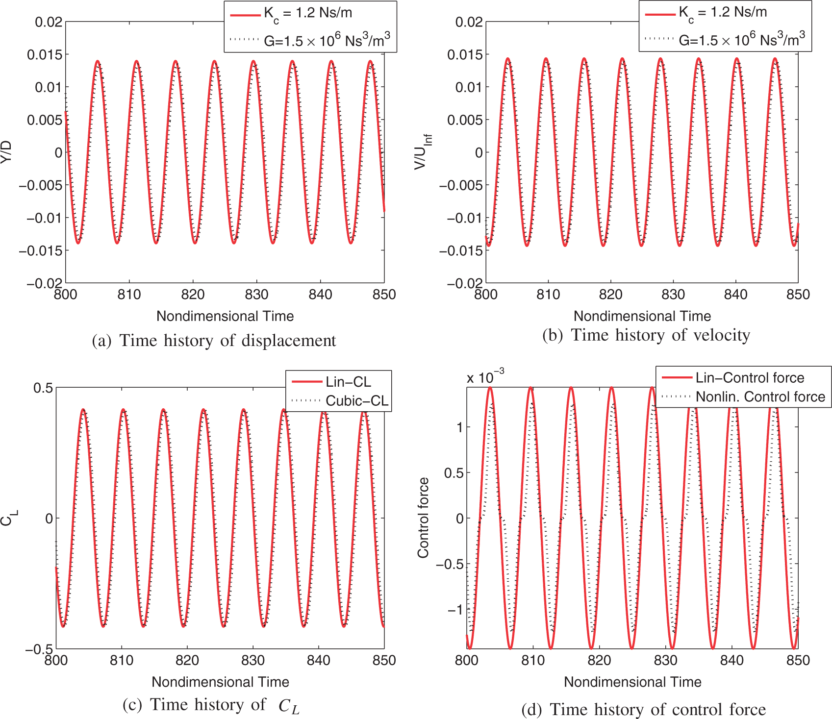

For the cubic velocity feedback controller, a reduced response is also observed in the whole range of synchronization. The effect of the gain G of the nonlinear velocity feedback controller on reducing the peak response amplitude is similar to that of the linear controller. For example, when Re = 105, an amplitude reduction of 26.2% is obtained when the cubic gain G = 100 Ns³/m³. Reductions of 42.36% and 96% are obtained when G = 300 Ns³/m³ and 1.0 × 10⁶ Ns³/m³, respectively, as shown in Figure 4(b).

Figure 5 shows time histories of the cylinder displacement for different linear and nonlinear control gains. Comparing the time trace of the uncontrolled case (i.e. K _c = 0 and G = 0) with those of the controlled cases (i.e. K _c ≠ 0 and G ≠ 0), we conclude that the oscillation amplitudes of the cylinder decrease as the gain of either of the two controllers is increased.

Figure 5.

Time histories of the cylinder transverse displacement for (a) the linear controller and (b) the nonlinear controller for different gains when Re = 106.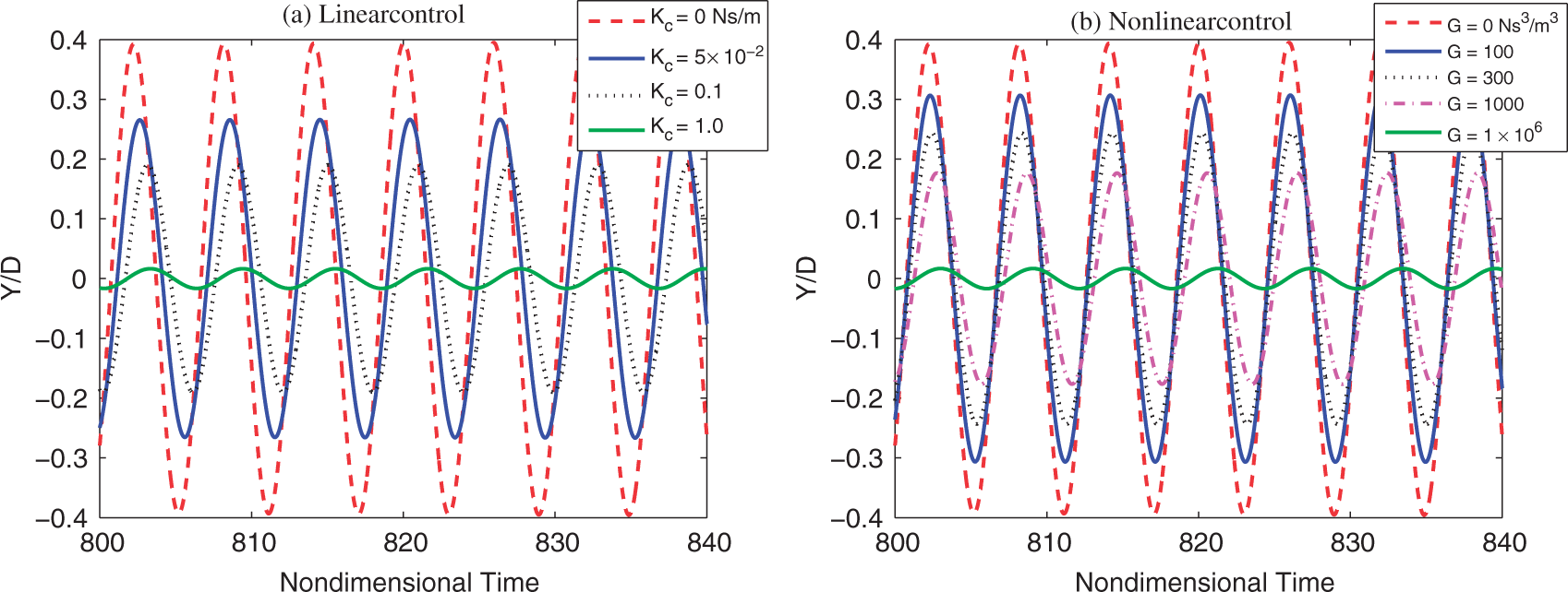

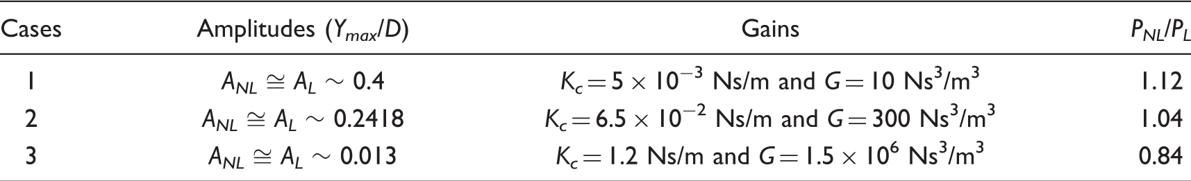
4. Power comparison and optimal control

To assess the effectiveness of both controllers, we performed a comparison between the power needed to suppress the oscillation amplitude of the cylinder to the same level. Three cases of the two controllers that yield the same level of oscillation amplitude are considered. In Case 1, we compare the results for K _c = 5 × 10⁻³ Ns/m and G = 10 Ns³/m³ when Re = 106. The oscillation amplitude of the cylinder is reduced to about Y _max/D ∼ 0.4 using either of the two feedback controllers, as shown in Figure 6(a). The associated velocity of the cylinder follows very closely that of the displacement for both cases, as shown in Figure 6(b). Moreover, the lift coefficient presented in Figure 6(c) oscillates around a zero mean with a peak value of about 1.25. All of these time histories show a steady-state periodic behavior and have a dominant frequency, the cylinder natural frequency. The feedback control force is plotted for both of the linear $((K_{c} / M f_{n} U_{r}) \overset{\cdot}{Y} *)$ and nonlinear $((G f_{n} D 2 U_{r} / M) \overset{\cdot}{Y} * 3)$ controllers in Figure 6(d). Inspecting this plot, we note that the cubic velocity feedback controller needs more force than the linear one. This is expected because the displacement and velocity amplitudes remain very high. The time series also shows a third harmonic in the nonlinear control force.

Figure 6.

Time histories of the (a) displacement, (b) velocity, (c) lift coefficient, and (d) control force when K _c = 5.0 × 10⁻³ Ns/m and G = 10 Ns³/m³ when Re = 106.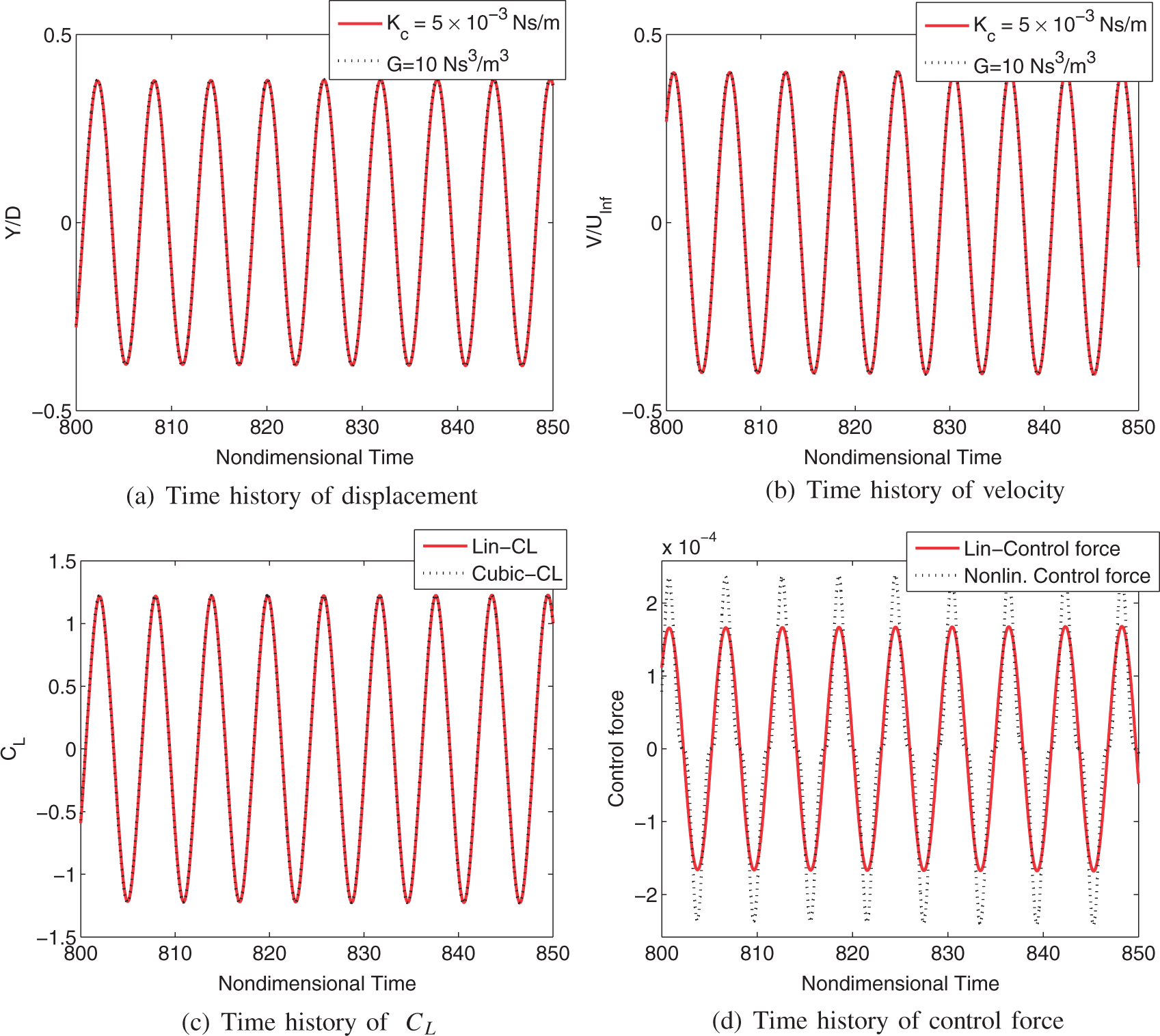

In Case 2, we compare the controlled cases for K _c = 6.5 × 10⁻² Ns/m and G = 300 Ns³/m³ when Re = 106. The oscillation amplitude for either of the two controllers is about Y _max D ∼0.24, as shown in Figure 7(a). Time histories of the velocity, lift coefficient, and control force are shown in Figure 7(b), (c), and (d), respectively. These plots show harmonic responses with a dominant frequency, the cylinder natural frequency. Figure 7(d) shows that the cubic velocity feedback force is again higher than the force needed in the case of the linear feedback controller. This is again due to the fact that the displacement and velocity amplitudes remain very large.

Figure 7.

Time histories of the (a) displacement, (b) velocity, (c) lift coefficient, and (d) control force when K _c = 6.5 × 10⁻² Ns/m and G = 300 Ns³/m³ when Re = 106.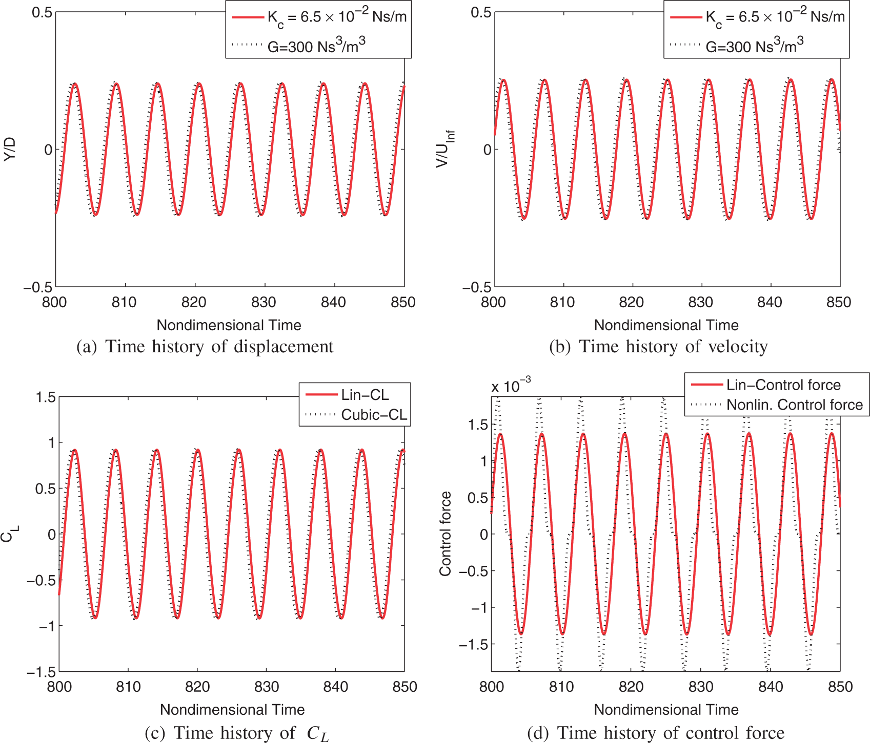

In Case 3, we compare the results for K _c = 1.2 Ns/m and G = 1.5 × 10⁶ Ns³/m³ considering the same Reynolds number (i.e. Re = 106 ). These gains are needed to obtain near-zero oscillation and velocity amplitudes, as shown in Figure 8(a) and (b). The lift coefficient, presented in Figure 8(c), oscillates around a zero mean with a peak value of 0.42. Inspecting Figure 8(d), we note that the force required for the nonlinear controller has a slightly lower amplitude than that of the linear one. This is due to the fact that the displacement and velocity amplitudes are very low.

4.1. Theoretical explanations

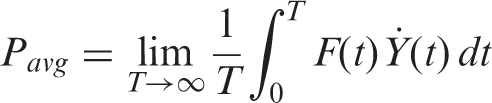
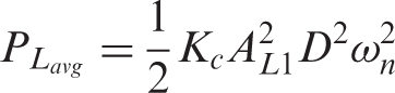
The linear control force is $F_{L} = - K_{c} \overset{\cdot}{Y}$ and the oscillation can be expressed as Y = DA ₁ cos(ω_n t + φ₁) + DA ₃ cos(3ω_n t + φ₃) where ω_n = 2πf _n, f _n is the dimensional natural frequency of the cylinder, and A _L1 and A _L3 are, respectively, the amplitudes of first and third harmonics of the nondimensional cylinder displacement. Inspecting Figure 9, we note that the amplitude of the third harmonic is very small compared with that of the first harmonic. Hence, the cylinder displacement can be approximated by DA ₁ cos(ω_n t + φ₁). The average power is given by

P_{avg} = lim_{T \to \infty} 1 T \int_{0}^{T} F (t) \overset{\cdot}{Y} (t) dt

For the case of linear velocity feedback, this average is equal to

P_{L_{avg}} = 12 K_{c} A_{L 1}^{2} D 2 ω_{n}^{2}

(14)

where A _L1 is the nondimensional oscillation amplitude of the cylinder for the linear velocity feedback controller. In the case of the nonlinear controller, the required force is

- G \overset{\cdot}{Y} 3

. The average required power is then equal to

P_{{NL}_{avg}} = 38 G A_{NL 1}^{4} D 4 ω_{n}^{4}

(15)

where A _NL1 is the nondimensional oscillation amplitude of the cylinder for the cubic velocity feedback controller. The ratio of the average powers required for the nonlinear and linear controllers is then written as

P_{{NL}_{avg}} P_{L_{avg}} = 34 G K_{c} A_{NL 1}^{4} A_{L 1}^{2} D 2 ω_{n}^{2}

(16)

Figure 9.

Power spectrum of the displacement of a rigid cylinder oscillating in the cross-flow direction when Re = 106 and G = 300 Ns³/m³.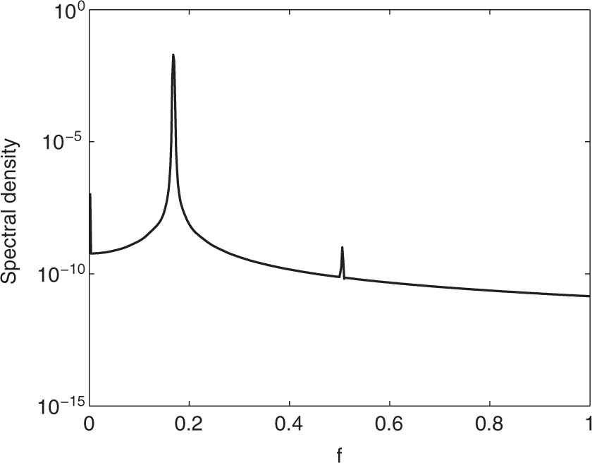

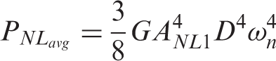
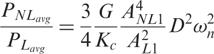
It is clear that the ratio depends strongly on the desired controlled amplitude and the required gains. The ratios of the average power of the considered three cases are presented in Table 1. We note that the linear controller is more appropriate if relatively large controlled amplitudes are allowed. However, for cases where very small controlled amplitudes are desired, the nonlinear controller is more efficient. As a matter of fact, the power level needed can be reduced significantly if a nonlinear controller with a relatively large gain is used. This is evident from Figure 10, where the controlled power for both controllers is plotted as a function of the controlled amplitude.

Figure 10.

Comparison between the linear and nonlinear control powers as a function of the controlled amplitude when Re = 106.

Table 1.

Comparison of the power requirements for the linear and nonlinear controllers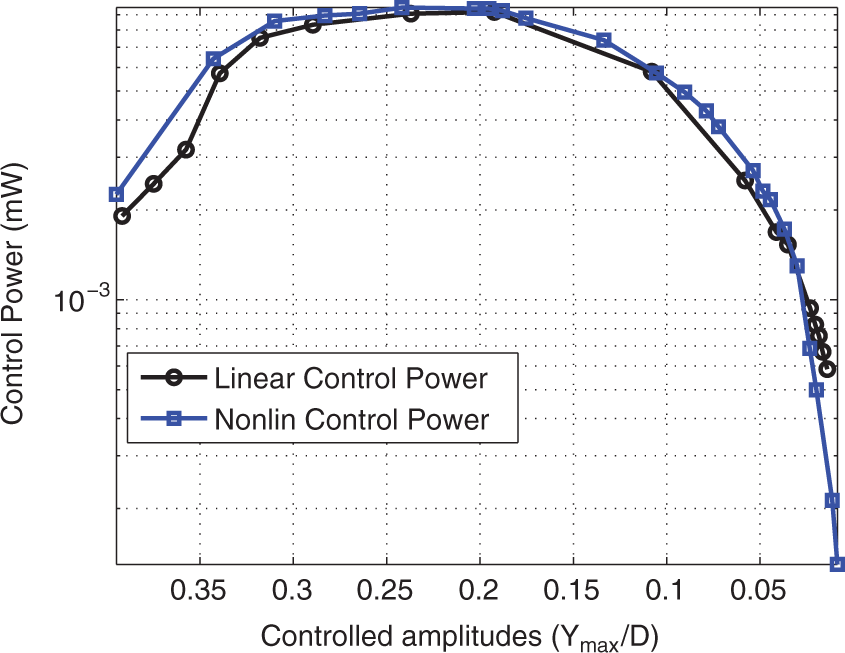

Cases	Amplitudes (Y _max/D)	Gains	P _NL/P _L
1	A _NL ≅ A _L ∼ 0.4	K _c = 5 × 10⁻³ Ns/m and G = 10 Ns³/m³	1.12
2	A _NL ≅ A _L ∼ 0.2418	K _c = 6.5 × 10⁻² Ns/m and G = 300 Ns³/m³	1.04
3	A _NL ≅ A _L ∼ 0.013	K _c = 1.2 Ns/m and G = 1.5 × 10⁶ Ns³/m³	0.84

5. Conclusions

We investigated the effectiveness of linear and nonlinear velocity feedback controllers to suppress high-amplitude oscillations of an elastically mounted rigid cylinder. Each controller imparts an opposing force to the cylinder motion, thereby reducing its high-amplitude oscillations. The opposing force, in the case of the linear controller, is proportional to the velocity of the cylinder, while, in the case of the nonlinear controller, it is proportional to the cubic velocity of the cylinder. The results show that both control laws have a significant effect on the response of the cylinder and damp the high-amplitude oscillations of the cylinder in the synchronization regime. A comparison of the performance of the two controllers based on suppressing the oscillations to the same desired amplitude was performed. The results show that, for relatively allowed large controlled amplitudes, the linear velocity feedback controller is more efficient. On the other hand, for very small controlled amplitudes, the cubic velocity feedback controller is more efficient.

Footnotes

Funding

A Mehmood gratefully acknowledges the University of Engineering & Technology (UET) Peshawar, Pakistan for financial support during his graduate studies. Numerical simulations were performed on the Virginia Tech Advanced Research Computing - System X and HokieOne. The allocation grant and support provided by the staff is also gratefully acknowledged.

References

Bearman

(1984) Vortex shedding from oscillating bluff bodies. Annual Review of Fluid Mechanics 16: 195–222.

Williamson

CHK

Roshko

(1988) Vortex formation in the wake of an oscillating cylinder. Journal of Fluids and Structures 2: 355–381.

Williamson

CHK

(1996) Vortex dynamics in the cylinder wake. Annual Review of Fluid Mechanics 28: 477–539.

Williamson

CHK

Govardhan

(2004) Vortex-induced vibrations. Annual Review of Fluid Mechanics 36: 413–455.

Jauvtis

Williamson

CHK

(2004) The effect of two degrees of freedom on vortex-induced vibration at low mass and damping. Journal of Fluid Mechanics 509: 23–62.

Gabbai

Benaroya

(2005) An overview of modeling and experiments of vortex-induced vibration of circular cylinders. Journal of Sound and Vibration 282: 575–616.

Gad-el-Hak

(2000) Flow Control: Passive, Active and Reactive Flow Management, Cambridge: Cambridge University Press.

Choi

Jeon

W-P

Kim

(2008) Control of flow over a bluff body. Annual Review of Fluid Mechanics 40: 113–139.

Zdravkovich

(1981) Review and classification of various aerodynamic and hydrodynamic means for suppressing vortex shedding. Journal of Wind Engineering and Industrial Aerodynamics 7: 145–189.

10.

Walshe

Wootton

(1979) Preventing wind-induced oscillations of structures of circular section. Proceedings of the Institution of Civil Engineers 47: 1–24.

11.

Baz

(1991) Active control of flow-induced vibrations of a flexible cylinder using direct velocity feedback. Journal of Sound and Vibration 146: 33–45.

12.

Govardhan

Williamson

CHK

(2006) Defining the ‘modified Griffin plot’ in vortex-induced vibration: revealing the effect of Reynolds number using controlled damping. Journal of Fluid Mechanics 561: 147–180.

13.

Skop

Griffin

(1973) A model for the vortex-excited resonant response of bluff cylinders. Journal of Sound and Vibration 27: 225–233.

14.

Nayfeh

Owis

Hajj

(2003) A model for the coupled lift and drag on a circular cylinder. ASME International Design Engineering Technical Conferences, Computers and Information in Engineering Conference. Chicago, IL.

15.

Abdelkefi

Hajj

Nayfeh

(2012) Phenomena and modeling of piezoelectric energy harvesting from freely oscillating cylinders. Nonlinear Dynamics 70: 1377–1388.

16.

Akhtar

Nayfeh

(2008) On controlling the bluff body wake using a reduced-order model. Proceedings of the 4th Flow Control Conference. Seattle, WA: paper AIAA-2008-4189 23–26 June.

17.

Blevins

(1985) The effect of sound on vortex shedding from cylinders. Journal of Fluid Mechanics 161: 217–237.

18.

Ffowcs Williams

Zhao

(1988) The active control of vortex shedding. Journal of Fluids and Structures 3: 115–122.

19.

Huang

(1996) Feedback control of vortex shedding from a circular cylinder. Experiments in Fluids 20: 218–224.

20.

Mittal

Iaccarino

(2005) Immersed boundary methods. Annual Review of Fluid Mechanics 37: 239–261.

21.

Hirt

Amsden

Cook

(1974) An arbitrary Lagrangian–Eulerian computing method for all flow speeds. Journal of Computational Physics 14: 227–253.

22.

Blackburn

Henderson

(1999) A study of two-dimensional flow past an oscillating cylinder. Journal of Fluid Mechanics 385: 255–286.

23.

Akhtar

(2008) Parallel Simulations, Reduced-order Modeling, and Feedback Control of Vortex Shedding using Fluidic Actuators. PhD thesis, Blacksburg, VA: Virginia Tech 2008.

24.

Akhtar

Nayfeh

Ribbens

(2009a) On the stability and extension of reduced-order Galerkin models in incompressible flows: a numerical study of vortex shedding. Theoretical and Computational Fluid Dynamics 23: 213–237.

25.

Akhtar

Marzouk

Nayfeh

(2009b) A van der Pol–Duffing oscillator model of hydrodynamic forces on canonical structures. Journal of Computational Nonlinear Dynamics 4: 041006.

26.

Carnahan

Luther

Wilkes

(1969) Applied Numerical Methods, New York: John Wiley & Sons, Inc. 1969.

27.

Anagnostopoulos

Bearman

(1992) Response characteristics of a vortex-excited cylinder at low Reynolds numbers. Journal of Fluids and Structures 6: 39–50.

28.

Yang

Preidikman

Balaras

(2008) A strongly coupled, embedded-boundary method for fluid–structure interactions of elastically mounted rigid bodies. Journal of Fluids and Structures 24: 167–182.

29.

Schulz

Kallinderis

(1998) Unsteady flow structure interaction for incompressible flows using deformable hybrid grids. Journal of Computational Physics 143: 569–597.