
Abstract
We investigate the validity and accuracy of using assumed modes methods to estimate the effective nonlinearities of vibration modes. For this purpose, a problem concerning the nonlinear response of a linearly tapered cantilever beam is considered. Since, in the selected example, the linear eigenvalue problem cannot be solved analytically for the exact mode shapes, an approximate set is required to discretize the partial differential equation governing the beam's motion. To approximate the mode shapes, three methods are utilized: (i) a crude approach, which directly utilizes the linear mode shapes of a regular (untapered) cantilever beam; (ii) a finite-element approach wherein the mode shapes are obtained in ANSYS, then fitted into orthonormal polynomial curves while minimizing the least square error in the modal frequencies; and (iii) a Rayleigh–Ritz approach which utilizes a set of orthonormal trial basis functions to construct the mode shapes as a linear combination of the trial functions used. Upon discretization, the modal frequencies, the geometric and inertia nonlinearity coefficients, as well as the effective nonlinearities of the first three vibration modes are compared for eight beams with different tapering. It is shown that, even when the modal frequencies are well-approximated using the three methods, a large discrepancy is observed among the estimates of the inertia, geometric and, thereby, effective nonlinearities of the structural modes. In fact, when using the modal frequencies as a convergence measure for assumed modes methods, inaccurate, and sometimes, erroneous predictions of the effective nonlinearities can be obtained. As a result, this paper recommends that a stricter measure based on the convergence of the nonlinear coefficients be implemented for discretizing a nonlinear system using approximate mode shapes.
1. Introduction
In the last two decades, the emergence and evolution of micro-electromechanical systems (MEMSs) and vibratory energy harvesting has renewed the interest in the nonlinear dynamics of structures. Such systems usually have complex shapes, nontraditional excitation mechanisms (electrostatic and electromagnetic), and are designed to undergo larger deflections, making them prone to behave nonlinearly. Examples include, but are not limited to, electrostatic micro-switches (Younis et al., 2003), atomic force microscopes Lee et al. (2002); Rutzel et al. (2003), mechanical micro-filters (Hammad et al., 2010), micro-sensors (Abdel-Rahman et al., 2003), and nonlinear energy harvesters (Mann and Sims, 2008; Masana and Daqaq, 2011b).
In general, nonlinearity can either improve or worsen performance. With that, a measure of its strength (strong or weak) and nature (softening or hardening) is quite important. Such a measure, also known as the effective nonlinearity, has been established and used by various researchers to quantify the influence of nonlinearity on the response of structures (Lacarbonara et al., 1998; Nayfeh and Mook, 1979; Nayfeh and Lacarbonara, 1997; Abdel-Rahman et al., 2003; Masana and Daqaq, 2011a; Emam and Nayfeh, 2004; Younis and Nayfeh, 2003; Zhang et al., 2002). It has been shown that the effective nonlinearity is dependent on the geometric and material parameters of the system and can be different for different vibration modes. For instance, the effective nonlinearity of the first mode of a stainless-steel cantilever beam has been shown to be of the hardening nature whereas the second and third modes exhibit softening characteristics (Nayfeh and Pai, 2004).
To estimate the effective nonlinearity of a certain structural mode, it is common to seek an approximate analytical solution of the nonlinear partial differential equations (PDEs) and boundary conditions governing the dynamics of the structure. The method of multiple scales, among other perturbation techniques, is usually used for that purpose. The process usually goes as follows: after the PDEs and boundary conditions are derived, a discretization procedure is used to transform the system into an infinite set of nonlinear ordinary differential equations (ODEs). The set can then be truncated based on a convergence analysis. Subsequently, the method of multiple scales is used to seek an approximate analytical solution of the response. The effective nonlinearity of a given vibration mode can then be obtained under the assumption that the mode is not involved in an internal resonance or an external combination resonance with any of the other modes.
In the discretization, the mode shapes resulting from the linear eigenvalue problem (solution of the associated linear PDE and boundary conditions) are usually used as the orthonormal set of basis functions. However, when the structure of interest has a complex shape, the resulting linear PDE can be very hard to solve for the exact linear mode shapes (Caruntu, 2007; Hammad et al., 2010). In such instances, two approaches have been commonly utilized in the open literature. In the first approach, a Rayleigh–Ritz procedure that employs an arbitrary set of orthonormal basis functions is used to approximate the actual mode shapes of the structure. The number of functions in the trial set is increased until convergence of the modal frequencies is realized within a specified tolerance (Rao, 2007). While accurate, this approach can involve computational complexities especially when the response of the higher vibration modes is considered.
To alleviate this problem, a second approach has been recently adopted wherein finite-element methods (FEMs) are used to approximate the linear mode shapes of the structure. The mode shapes are then fitted into an orthonormal basis set that can be used in the discretization (Gabbay and Senturia, 2000; Hammad et al., 2010; Mehner et al., 2000; Sclaroff and Pentland, 1995). This technique has been gaining wider interest in the open literature due to its simplicity and its ability to generate modal shapes for complex structures and higher vibration modes, thereby reducing computational cost.
In this paper, we investigate the accuracy of using approximate mode shapes to estimate the effective nonlinearity of a given vibration mode. To that end, we consider the nonlinear vibrations of a cantilever beam tapered linearly along its width. To the best of the authors' knowledge, the associated linear eigenvalue problem cannot be solved exactly. Consequently, the exact linear mode shapes cannot be obtained and used in the discretization, requiring a set of approximate mode shapes. 1 Here, three approximation methods are used: (i) a crude approach which directly utilizes the known modes of a regular (untapered) beam to estimate the modal frequencies and effective nonlinearity; (ii) a finite-element approach wherein the linear mode shapes are obtained using ANSYS, then fitted into orthonormal polynomial curves; and (iii) a Rayleigh–Ritz approach which utilizes the mode shapes of the regular beam as an orthonormal trial set to construct the approximate mode shapes as a linear combination of the trial functions used. The effective nonlinearity coefficients of the first three structural modes for eight different beam tapering are then approximated using the three methods. A comparative analysis is presented to arrive at some conclusions regarding the accuracy of such techniques.
2. Problem formulation
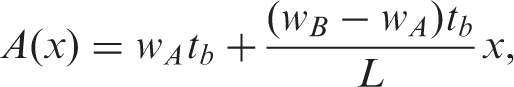
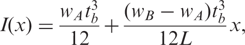
We consider the nonlinear dynamics of a tapered Euler–Bernoulli cantilever beam for which the cross-sectional area and moment of inertia vary across its length according to
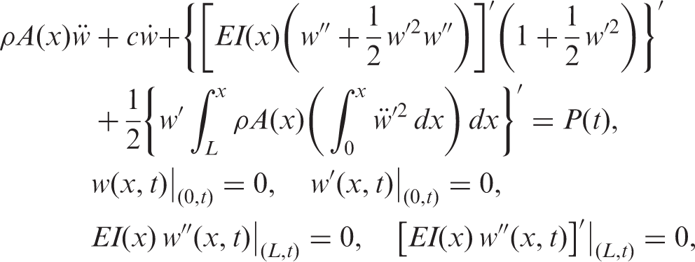
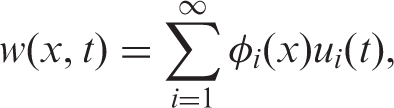
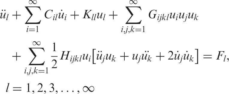
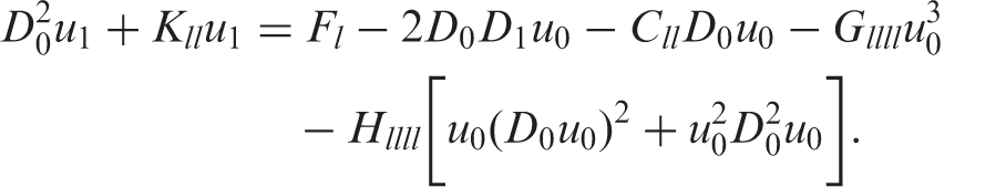
Owing to the nonlinearity, an exact analytical solution of Equation (3) cannot be attained easily. An approximate analytical solution can be obtained by discretizing the nonlinear PDE into a set of nonlinear ODEs. This can be realized by assuming a series solution of the form Rao (2007)
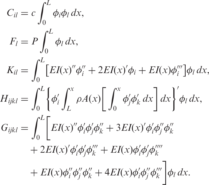
Substituting Equation (4) into Equation (3), multiplying by φ
l
(x) where l is a free index, integrating over the length of the beam, and using the orthonormality properties of the chosen basis set (see the Appendix for details), we obtain
3. Effective nonlinearity of a vibration mode
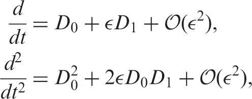
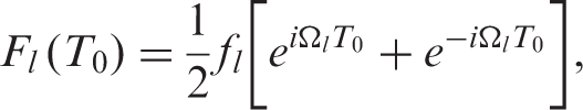
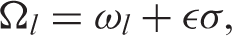
To obtain an expression for the effective nonlinearity of a given vibration mode, we utilize the method of multiple scales. We assume that the excitation frequency is close to the modal frequency of a given mode and that this mode is not involved in an internal resonance or an external combination resonance with any of the other modes, which allows us to adopt a single-mode representation of the dynamics.
2
We then expand the time dependence into multiple time scales as
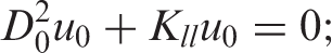
O(ε0):
O(ε):
The solution for the zeroth-order problem, Equation (11), can be written as


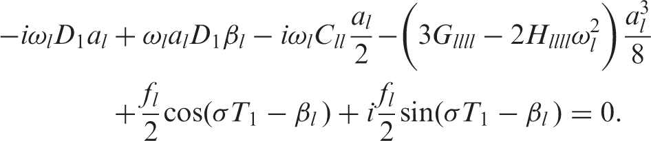
After separating real and imaginary parts of Equation (17), we obtain the following two modulation equations
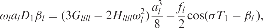
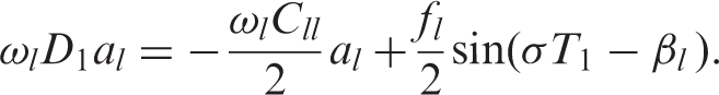
The cubic term in the phase equation, Equation (18a), is the only source of nonlinearity in the dynamics of this system. It can be easily shown that when this term vanishes, the linear problem can be recovered. With that, the coefficient multiplying
4. Assumed mode shapes
To estimate the effective nonlinearity of a given vibration mode using Equation (19), the mode shapes of the tapered beam should be determined first. However, since the linear eigenvalue problem associated with the system at hand cannot be solved analytically because the temporal and spatial parts cannot be easily separated, other, usually approximate mode shapes must be utilized. In what follows, we adopt three approaches of different accuracy to estimate the mode shapes and investigate their influence on effective nonlinearity.
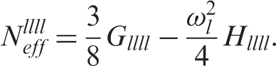
4.1. Regular cantilever beam mode shapes

Width in meters of the tapered cantilever beams.
Material and geometric properties.
Results obtained using regular (untapered) beam mode shapes.
4.2. Finite-element methods
Results obtained using a finite-element method (FEM). “ANS” represents frequencies obtained directly from ANSYS and “Freq” represents those obtained by curve fitting the mode shapes.
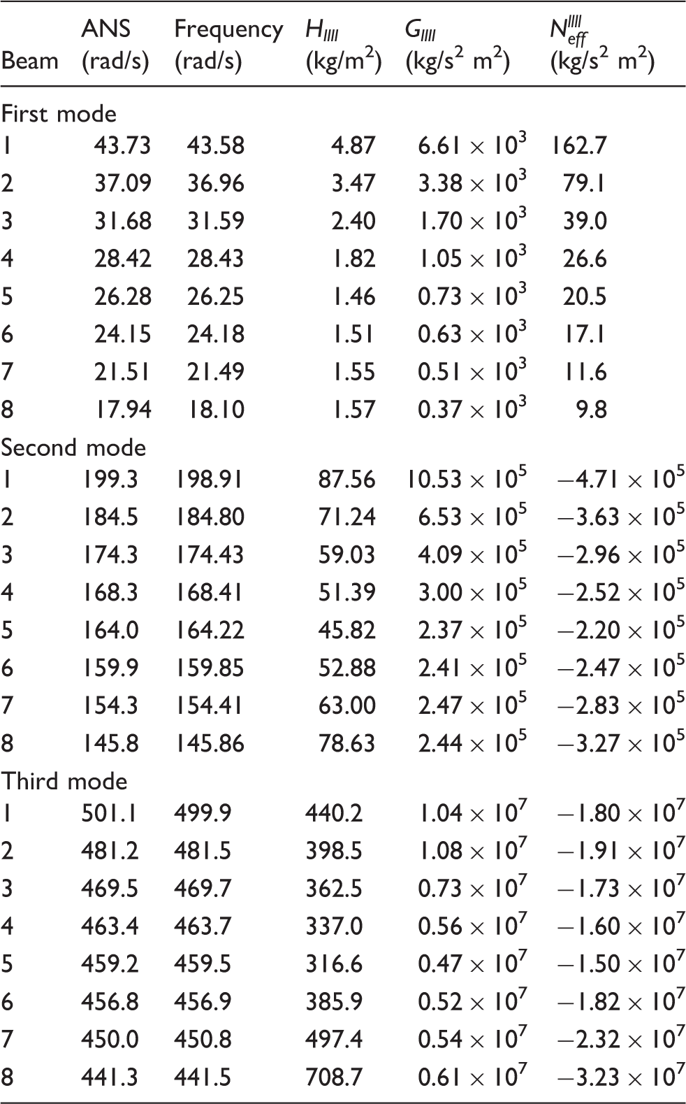
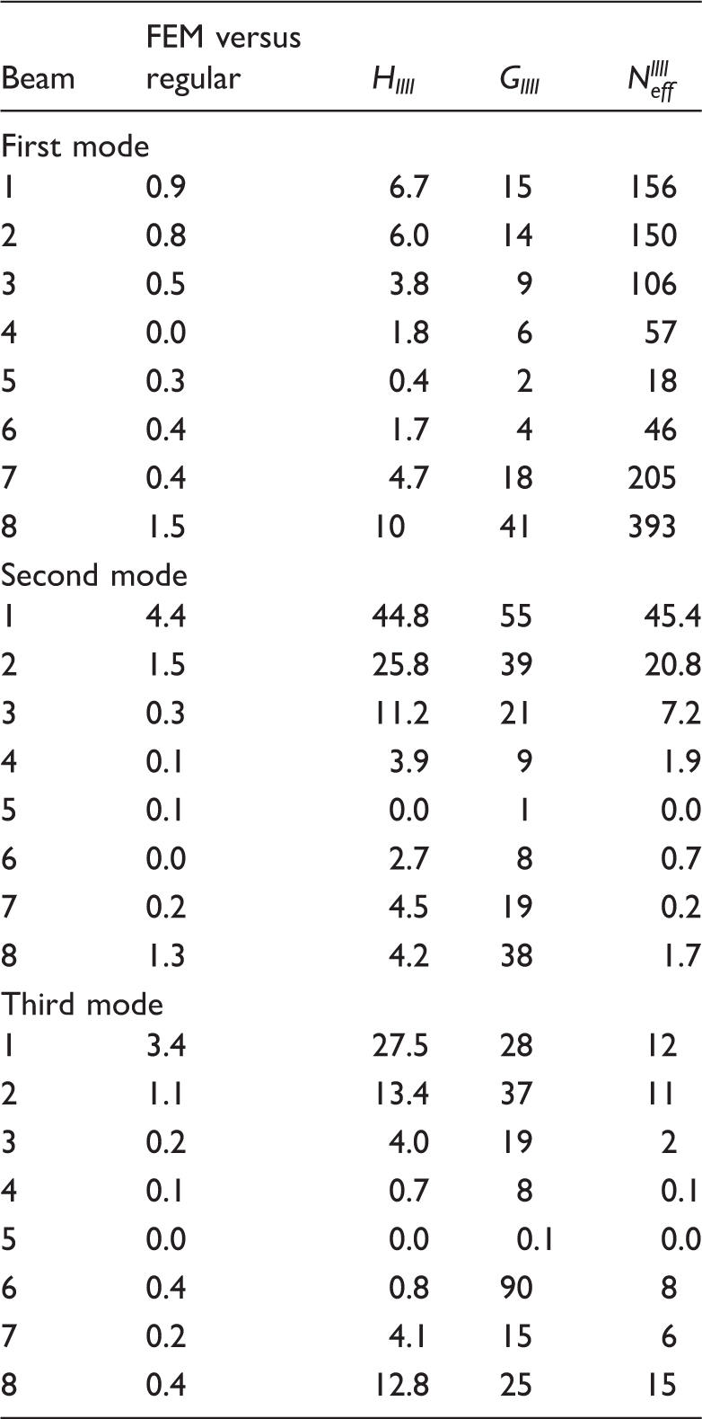
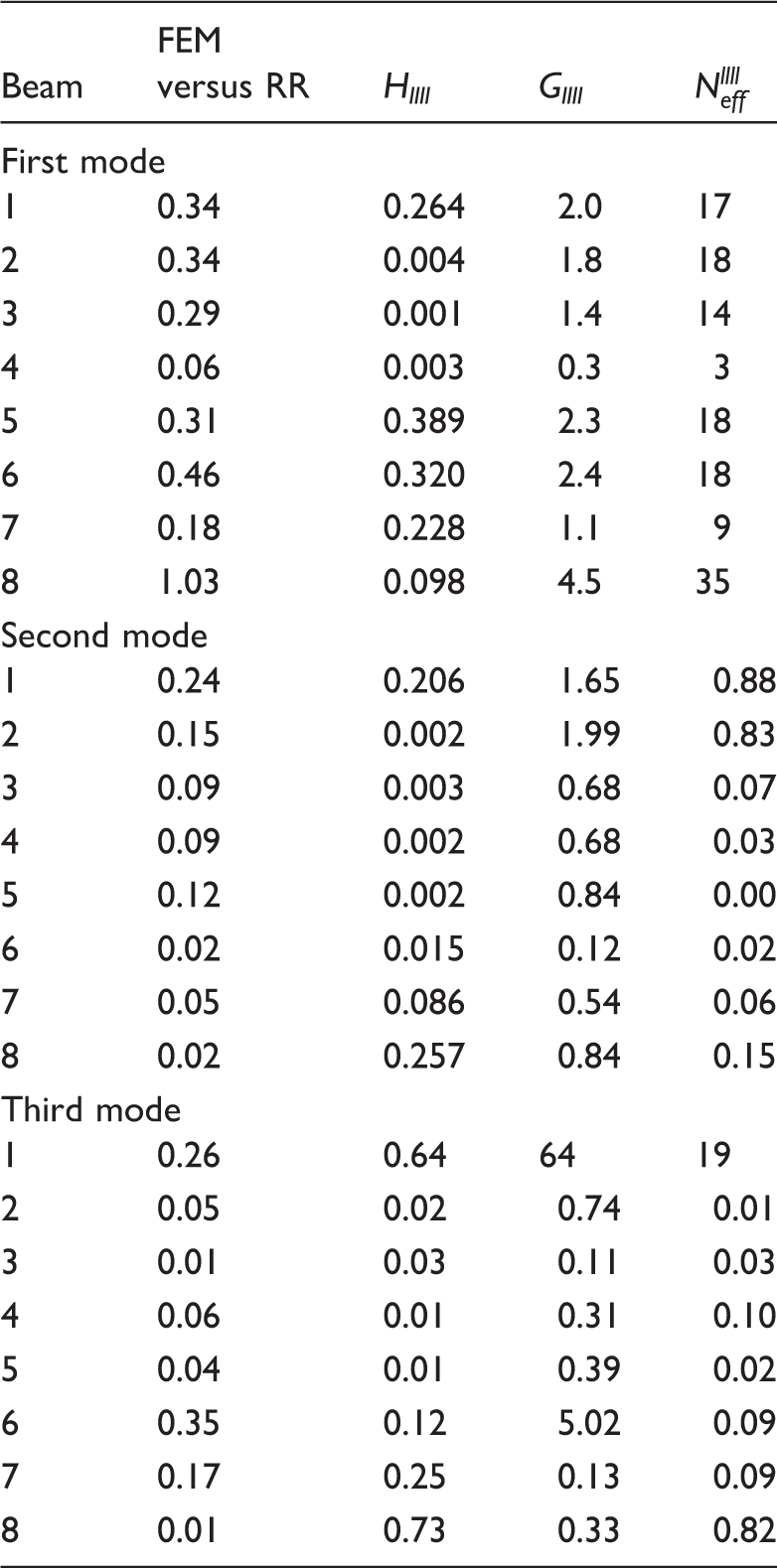
Absolute value of the relative difference between the FEM approach and the mode shapes of a regular beam. Frequency, inertia, geometric, and effective nonlinearities (%).
Although the modal frequencies are well estimated using both approaches, a large discrepancy is observed in the estimation of the effective nonlinearity, especially for beams with the larger tapering. The deviation, which can be as large as 400% (beam 8, first mode) is mainly due to discrepancies in estimating the geometric nonlinearity coefficient G
llll
. In fact, these deviations can be so large that, for some beam tapering, one method predicts a softening type behavior (negative effective nonlinearity) while the other predicts a hardening response (positive effective nonlinearity). This results in a completely different frequency response behavior for the first mode as shown in Figure 1(c). Such results are critical, especially knowing that the relative percentage difference in estimating the frequency does not exceed 1.5% for the first mode in the worst-case scenario. Based on the values of the modal frequencies, one can be tricked into assuming that the untapered mode shapes are sufficient to predict the nonlinear behavior of the beam. However, a quick comparison among the effective nonlinearity values reveals otherwise.
(a) Modal frequencies, (b) effective nonlinearity coefficients, and (c) frequency response behavior of beam number 2. Results are obtained for the first mode with viscous damping coefficient c = 0.07 kg/s and excitation force P = 1 N.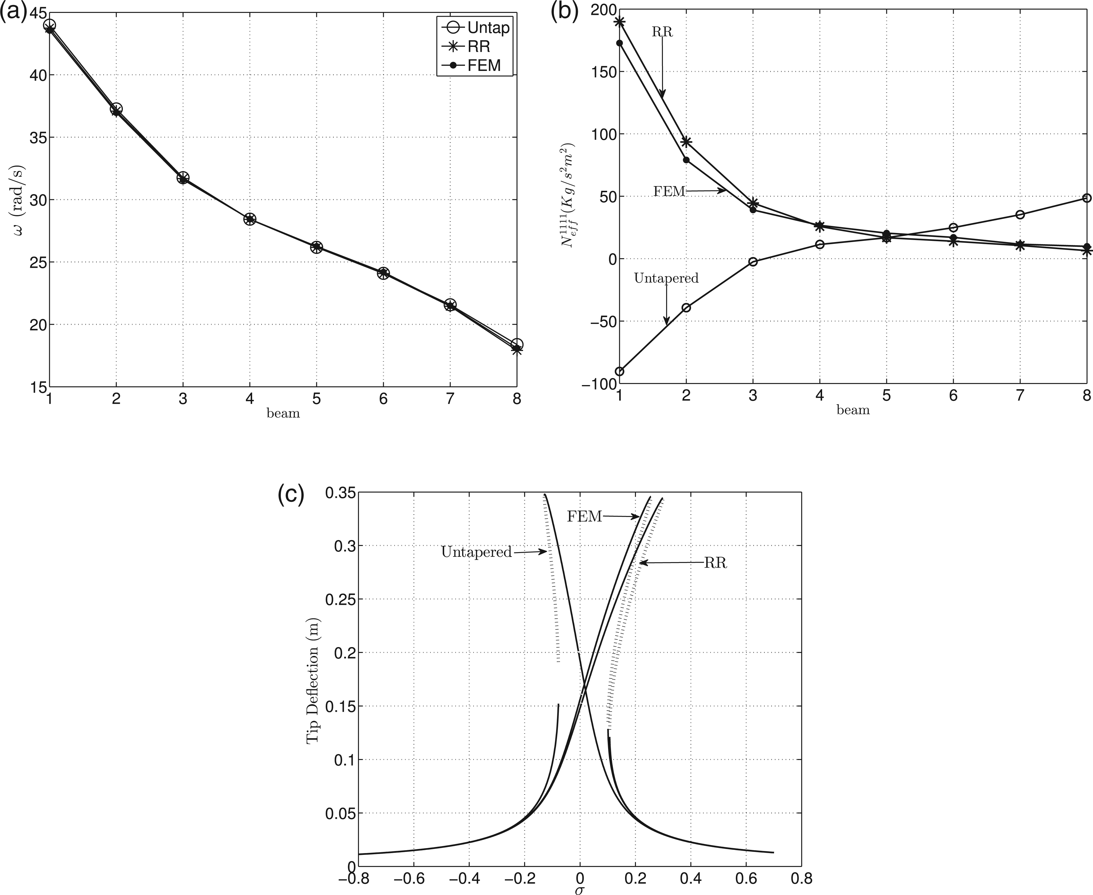
4.3. Rayleigh–Ritz approach
When the eigenvalue problem associated with a PDE and the boundary conditions cannot be solved exactly, it is a common practice to use the Rayleigh–Ritz approach to estimate the eigenvalues and associated mode shapes (Rao, 2007). In the Rayleigh–Ritz approach, a set of orthonormal trial functions that satisfy the boundary conditions are used as a basis set in the series discretization, Equation (4). Starting with one trial function, the linear eigenvalue problem is solved for an approximate first modal frequency and associated eigenvector. The number of trial functions or terms in the series is increased until that frequency converges within a specified tolerance. Once the frequency converges, the associated eigenvector is used to construct a global mode shape which is a linear combination of the trial functions used. This mode shape can then be used to calculate the integrals in Equation (6) and estimate the effective nonlinearity.
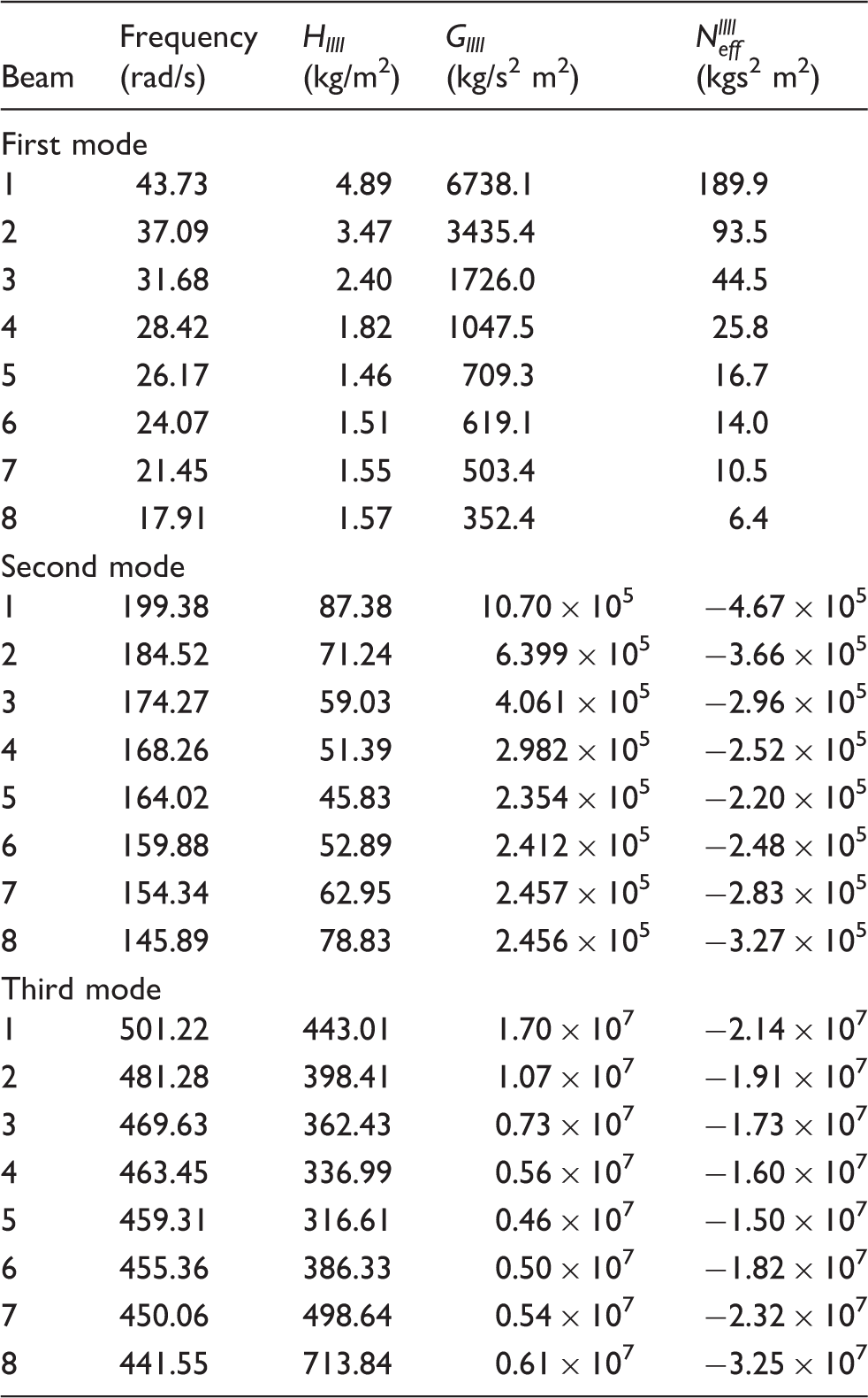
Results obtained using the Rayleigh–Ritz approach.
Absolute value of the relative difference between Rayleigh–Ritz and FEM approach. Frequency, inertia, geometric and effective nonlinearities (%).
Similar results are obtained for the second mode, Table 7. The frequency values are well-correlated with a maximum difference of 0.24% for beam 1. The error in the effective nonlinearity is around 1%, which is almost four times larger than the difference in the frequency estimate. The third mode results are shown in Table 7, with a maximum difference of 0.26% in the frequency estimates. The difference propagates to about 20% in the effective nonlinearity.
More qualitative conclusions can be drawn by inspecting Figures 1, 2, and 3, which depict the modal frequencies, the effective nonlinearity coefficients, and a sample frequency response curve for each of the first three vibration modes and each of the tapered cantilever beams. Figure 1(a) clearly illustrates that the first modal frequency is very closely estimated using the three methods such that no distinction between the curves can be visualized. On the other hand, when the untapered beam mode shapes were used to calculate the effective nonlinearity coefficient of the first mode as shown in Figure 1(b), the integrals yield positive and negative values depending on the direction and slope of the tapering. ANSYS and Rayleigh–Ritz are in good agreement, yielding a different trend where the effective nonlinearity is always positive (hardening type). This results in a completely different nonlinear frequency response behavior as clearly shown in Figure 1(c).
: (a) Modal frequencies, (b) effective nonlinearity coefficients, and (c) frequency response behavior of beam number 1. Results are obtained for the second mode with viscous damping coefficient 0.12 kg/s and excitation force 1.4 N. (a) Modal frequencies, (b) effective nonlinearity coefficients, and (c) frequency response curves of beam number 1. Results are obtained for the third mode with viscous damping coefficient 0.22 kg/s and excitation force 2 N.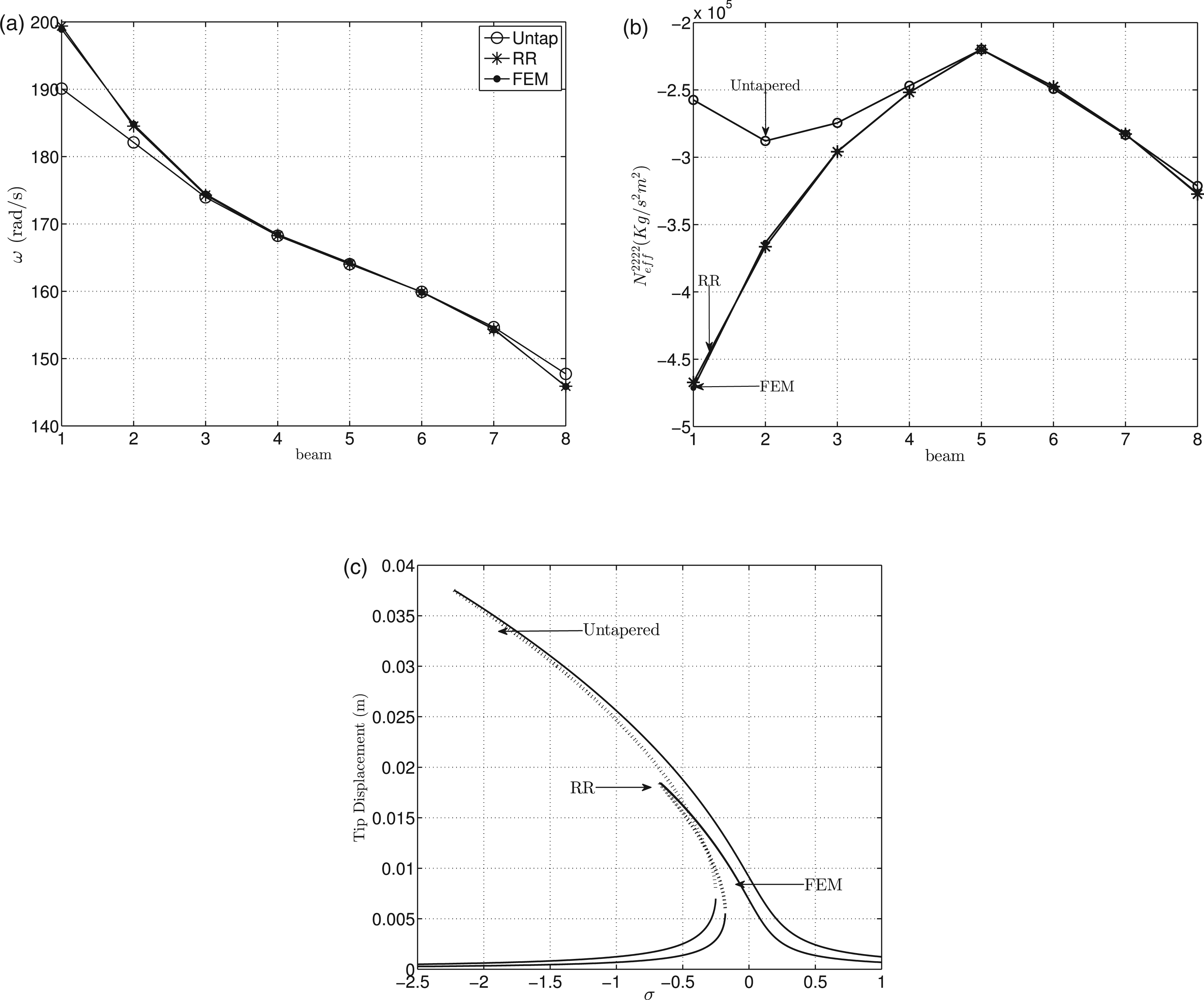
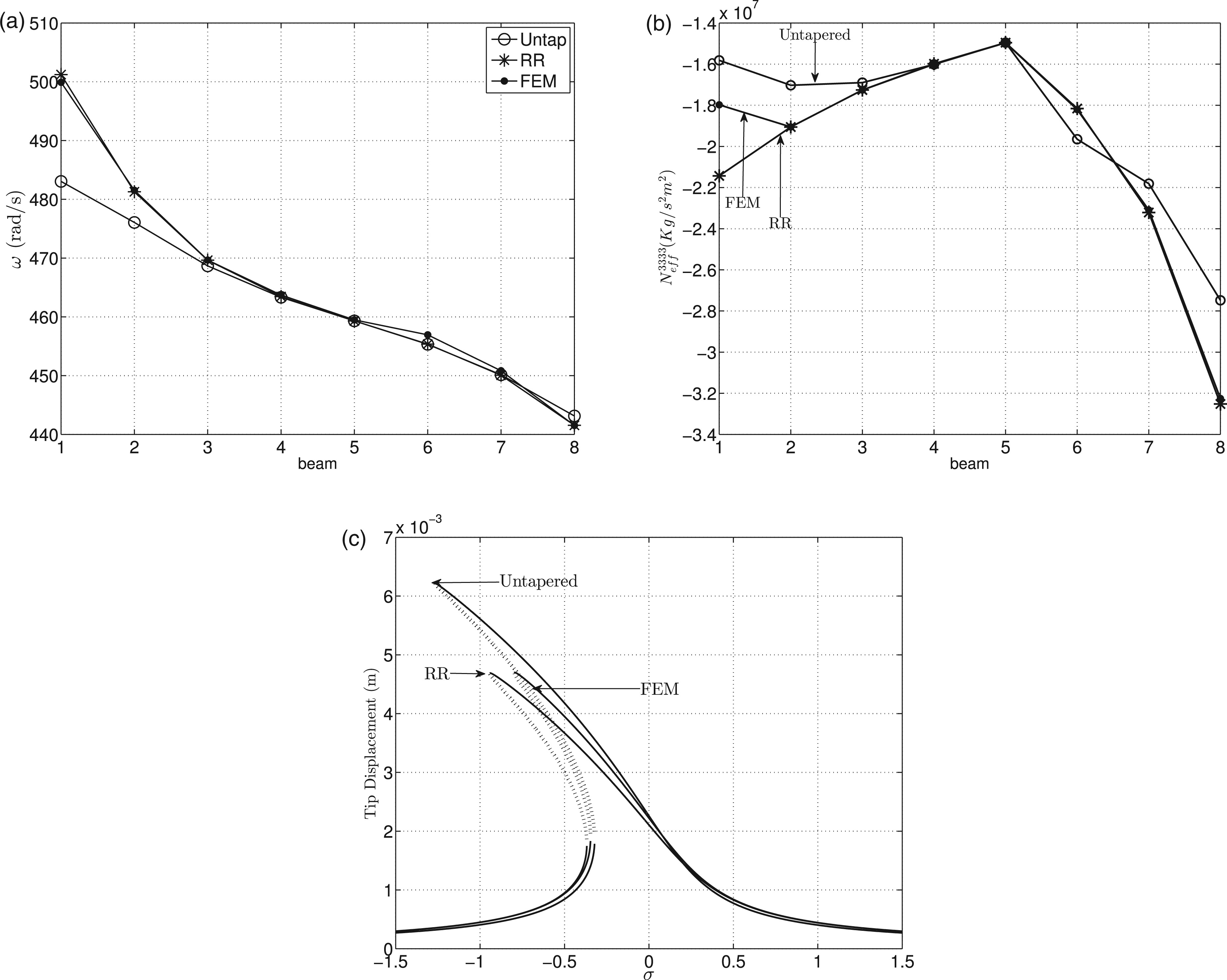
Although the general trend is mostly reflected, similar deviations can also be seen for the second and third modes, Figures 2(c) and 3(c). Such deviations are not only reflected in the degree by which the frequency response curves bend, but also in the amplitude of the steady-state response as shown in Figures 2(c) and 3(c). This indicates that the modal damping coefficients and the modal projections of the base excitation (Equation 6) are also not very well approximated using the regular mode shapes.
5. Convergence analysis
It is a common practice in the open literature to base the convergence of modal expansion techniques, such as the Rayleigh–Ritz method, on the convergence of the modal frequencies. In this study, convergence is measured by calculating the relative difference between the frequency values obtained using n trial functions and those using six trial functions. In other words, we express the percentage error as
(a) Convergence of the first modal frequency and (b) the effective nonlinearity coefficient with the number of trial functions for the first mode of beam 2. Convergence of the modal frequencies with the number of trial functions (%).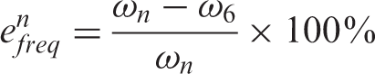
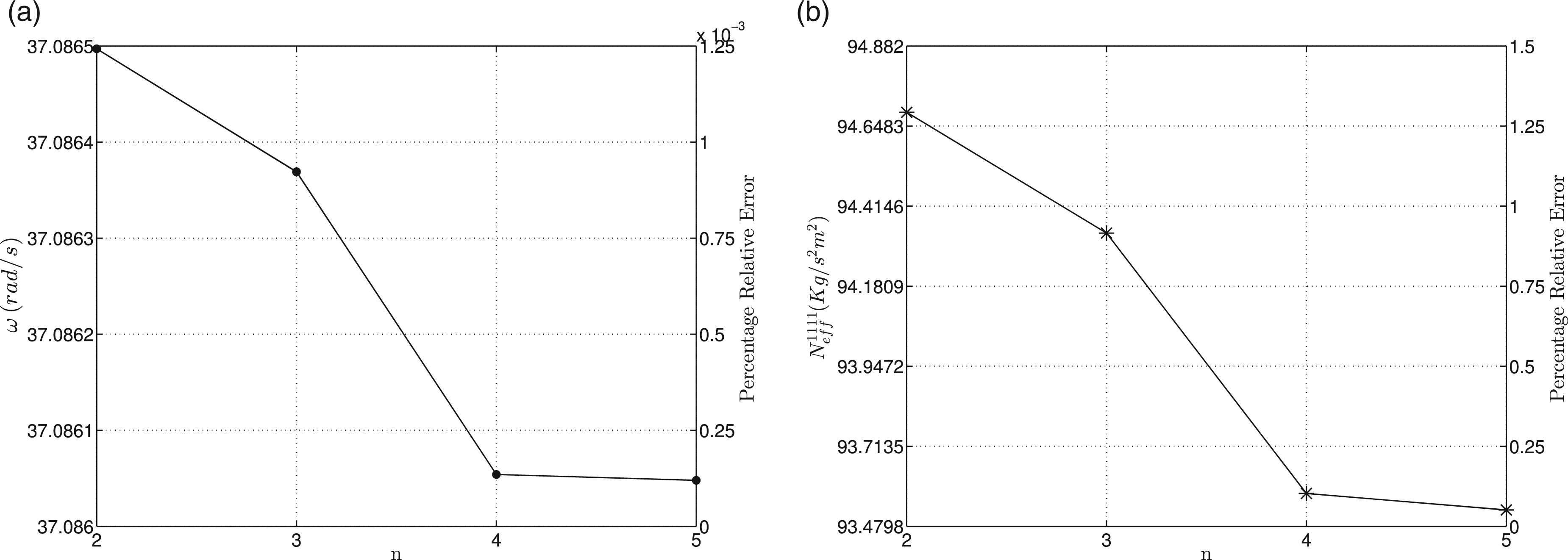
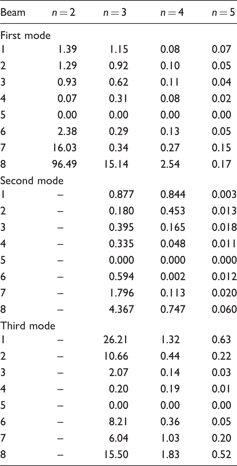
In this section, we explore how the convergence of the modal frequencies influences the convergence of the nonlinear parameters. Table 8 reveals that two trial functions are sufficient to estimate the first modal frequency with a maximum relative error of 0.42% for the beam with largest tapering (beam 8). The use of five trial functions drops the error to 0.0042%. Based on such results, it is safe to conclude that the linear dynamics of the first mode of the tapered beams is well described using two trial functions in the series discretization. Keeping more modes will only increase the complexity and computational cost of the analysis without significant improvement in the modal frequency estimates.
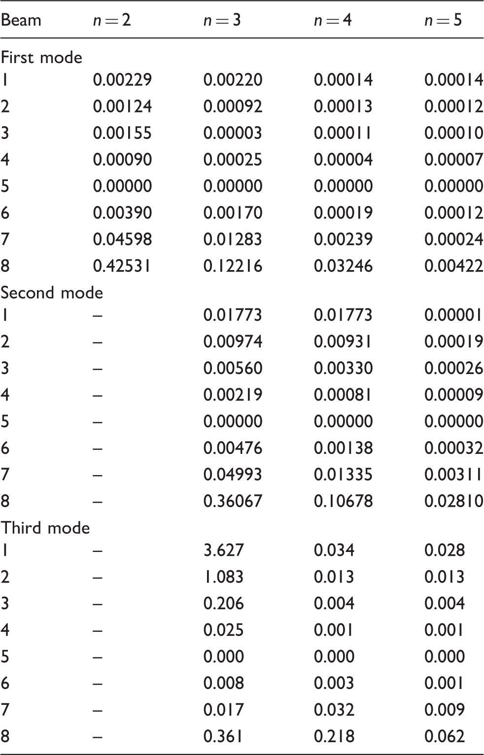
On the other hand, when inspecting the convergence of the effective nonlinearity coefficient of the first mode based on the same number of trial functions, see Table 9, a different conclusion is deduced. Using two trial functions to estimate the effective nonlinearity coefficient of the first mode for beam 8 yields 97% relative error. Increasing the number of trial functions to three, drops the error to about 15%, which is still very large compared with the error in the modal frequency estimates. The error drops to less than 1% only when five trial functions are utilized. Figure 5 depicts a comparison between the relative error in the frequency estimates and the associated effective nonlinearities as the number of trial functions is increased. The figure clearly demonstrates that, in order to estimate the effective nonlinearity with less than 1% relative error, the modal frequency should be estimated to within 0.001% of its best estimate. In other words, three orders of magnitude reduction in the error is necessary. Such results reveal that using the modal frequencies as a convergence measure for the assumed modes methods is not sufficient when the goal is to develop an accurate nonlinear reduced-order model. A stricter convergence measure based on the convergence of the nonlinear parameters should be implemented.
Convergence of the modal frequency and effective nonlinearity coefficient with the number of trial functions. Stars represent the effective nonlinearity values and dots represent modal frequencies. Results are obtained for the first mode of beam 2. Convergence of the effective nonlinearity coefficient with the number of trial functions (%).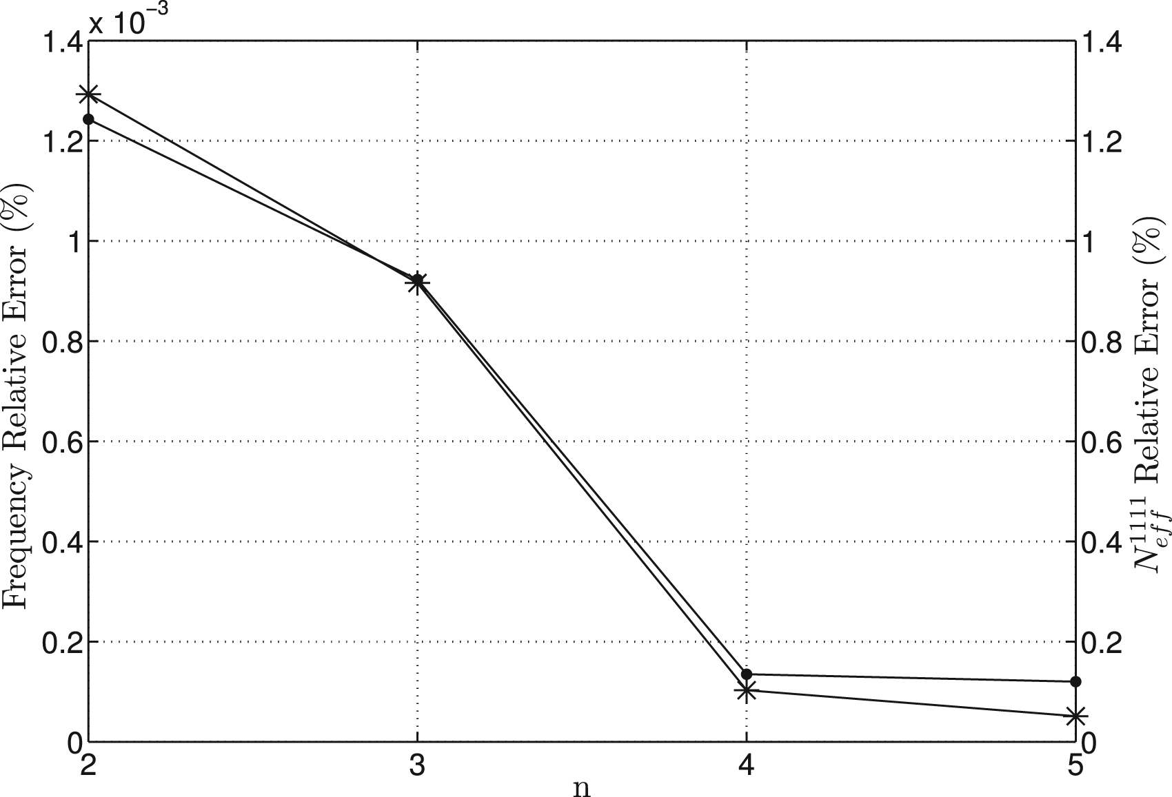
6. Conclusion
In this paper we have investigated the accuracy of using approximate mode shapes to estimate the effective nonlinearity of a given structural mode. To that end, the problem of estimating the effective nonlinearity of the structural modes associated with a cantilever beam tapered linearly along its width is considered. In this example, the linear eigenvalue problem cannot be solved exactly and, hence, the exact linear mode shapes cannot be obtained analytically to be used in the discretization. With that, three approximation methods are used: (i) a crude approach which directly utilizes the known modes of a regular (untapered) beam; (ii) a finite-element approach wherein the linear mode shapes are obtained using ANSYS, then fitted into orthonormal polynomial curves while minimizing the least square error in the modal frequencies; and (iii) a Rayleigh–Ritz approach which utilizes the mode shapes of the regular beam as an orthonormal basis function to construct the structural mode shapes as a linear combination of the trial functions used. The effective nonlinearity of the first three structural modes for eight beams with different tapering is then approximated using the three methods. A comparative analysis is presented clearly demonstrating that, while the modal frequencies are well approximated using the three methods, large discrepancies are observed in the estimation of the effective nonlinearity. In fact, in some instances, one method predicts a softening response while the other predicts a hardening response. This study concludes that convergence analysis of assumed mode methods should not be based on the modal frequencies when a nonlinear reduced-order model is sought. A stricter measure based on the convergence of the nonlinear parameters should be implemented.
Footnotes
Notes
Funding
This work was supported by CNPq - Brazilian National Council for Scientific and Technological Development and the Department of Mechanical Engineering at Clemson University.