Analytical study on in-plane free vibration of a cable network with straight alignment rigid cross-ties

Abstract

Using cross-ties is one of the effective countermeasures to suppress unfavorable bridge stay cable vibrations. It has been successfully applied in the field. However, dynamic behavior of cable networks is still not clearly understood, which hinders the development of a more efficient design. The current paper aims at extending the existing analytical studies on in-plane free vibration of cable networks by developing closed-form modal solutions for a wider series of cases, in particular for general cable networks consisting of n horizontally laid main cables interconnected transversely with a single line of rigid cross-ties. The validity of these analytical modal solutions is verified by independent finite element simulations. These closed-form modal solutions offer a clear elucidation of the mechanics underlying various modal behaviors observed in cable networks of different layout and structural properties. In addition, based on the proposed analytical formulation, the important system parameters of cable networks are identified. The unique features associated with cable networks of a number of specific configurations are investigated and discussed.

Keywords

Cable-stayed bridge cable network cross-tie cable vibration vibration control

1. Introduction

One main achievement in the recent advancement in bridge engineering is the design of cable-stayed bridges with much longer span length due to the ambitions of humans to cross wider spaces and the rapid development of materials and technology. Lightweight structural components and the use of longer spans result in more slender elements and structures that are susceptible to vibrations under various types of dynamic excitations. A typical example is the cables on cable-stayed bridges. Mainly due to their high flexibility, light mass and very low inherent damping, when subjected to various environmental factors such as wind, stay cables are unable to dissipate much of the excitation energy and are thus vulnerable to dynamic excitations. In addition, the nonlinear interaction between the motions of the cable and bridge deck can also lead to very large amplitude cable vibrations (e.g. Lilien and Pinto da costa, 1994; Macdonald and Georgakis, 2002; Caetano and Cunha, 2003; Sun et al., 2003). These unfavorable cable motions would cause problems related to structural safety and user discomfort.

Different solutions have been used on site to suppress undesired cable vibrations. Surface treatment is applied to cables to change their aerodynamic features (Matsumoto et al., 1992; Zhan et al., 2008). Mechanical types of solutions, including installation of external dampers and connection of a few cables by cross-ties, have also been implemented on site with different levels of effectiveness. The structural behavior of a cable when attached transversely with an external damper and the optimum design of such a cable-damper system have been extensively studied by many researchers (e.g. Pacheco et al., 1993; Krenk, 2000; Tabatabai and Mehrabi, 2000; Main and Jones, 2002; Fujino and Hoang, 2008; Cheng et al., 2010). However, the mechanism of the cross-tie solution is not yet well understood. When cross-ties are applied on site, the cables that are vulnerable to (or have experienced) large amplitude vibrations are connected to their neighboring cables through transverse secondary cables or cross-ties to form a cable network. Such a strategy aims at reducing the effective length of the problematic cable to increase its in-plane stiffness and thus natural frequency. Besides, the adoption of cross-ties may add extra damping to the target cable, which would also help to suppress vibrations. The cable sag variation among cables of different lengths is found to be reduced with the introduction of cross-ties as well (Gimsing and Georgakis, 1993).

So far, cross-ties have been successfully used on a number of cable-stayed bridges to control cable vibrations (e.g. Virlogeux, 1998; Caracoglia and Jones, 2005b; Kumarasena et al., 2007). After installing the cross-ties, no problematic cable vibrations have been reported. However, studies on the dynamic behavior of this type of cable network system are still limited.

Ehsan and Scanlan (1989) used the finite element approach for the solution of a three-dimensional cable network problem and studied the redistribution of oscillation energy in a cable network consisting of a number of stay cables connected by cross-ties. According to their study, the main function of the cross-ties in a cable network is to help transfer energy from a problematic cable to its neighbors.

Virlogeux (1998) described the unexpected behavior of cross-ties on the Normandie Bridge in France where one of the cross-ties was broken. It was not clear what caused the failure of this cross-tie. However, when these cross-ties were replaced by stronger ones with higher tension, the performance was found to be satisfactory. In another case reported by the same author, the installation of extremely low damping cross-ties was found to successfully suppress the rain–wind-induced vibrations of bridge stay cables.

Yamaguchi and Nagahawatta (1995) performed a set of physical tests on a simple cable network, of which two main cables of different lengths were connected through two transverse cross-ties symmetrically. It was found that the fundamental frequency of the cable network was higher than that of the top individual main cable (the longer one) and increased monotonically with the prestress in the cross-tie. The modal damping of the cable network was always greater than that of a single main cable without cross-tie. This modal damping increment was found to be more significant when more flexible (soft) cross-ties were used.

Caracoglia and Jones (2005a) developed an analytical procedure to study the in-plane free vibration of a cable network. In the formulation, the taut cable assumption was applied to the main cables and the cross-tie was simplified as either a rigid rod or a linear spring. Closed-form modal solutions were obtained for a few simple two-cable networks (Caracoglia and Jones, 2005a), whereas when extending to a more complicated cable network on a real cable-stayed bridge (Caracoglia and Jones, 2005b), the analytical approach was implemented numerically. In a more recent work (Caracoglia and Zuo, 2009), this analytical procedure was applied to cable networks of different configurations to determine the effectiveness of the cross-tie solution. It is worth noting that cable networks on real bridges generally consist of more than two stay cables. Numerically simulating its dynamic behavior would not allow a clear identification of important system parameters. In addition, the high cost associated with reconstruction of numerical model would limit the capability of the approach for an extensive parametric study.

Bosch and Park (2005) simulated the performance of a group of stay cables connected by cross-ties using the finite element software SAP 2000. Interestingly, it was found that the effectiveness of the cross-ties depended on their deployment geometry, the quantity, the size, and the anchorage conditions with the main cables. It was observed from the numerical simulation that when cables were connected by transverse cross-ties, vibration modes densely populated over a narrow band of frequency range would be induced. In addition, it was found that the combined use of cross-ties and external dampers would not necessarily produce the sum of the benefits when they are used separately.

In an experimental study by Sun et al. (2007), a scaled cable network model of three main cables connected by a transverse cross-tie was tested. The effects of different factors, such as the cross-tie stiffness, the tensioning method, and the pretension of the cross-ties, were evaluated. It was found that while the stiff type of cross-tie mainly contributed to enhance the in-plane stiffness of a cable network and thus its modal frequencies, the soft type of cross-tie is more effective in increasing the system damping.

A simplified analytical model was proposed recently by Zhou et al. (2011) to study the free vibration of a cable network. Only the target cable was included in the model, and the effects of cross-ties were modeled as linear springs.

In the majority of previous studies, either physical tests or numerical simulations were conducted to explore the dynamic behavior of a cable network. To the knowledge of the authors, very few studies (e.g. Caracoglia and Jones, 2005a, 2005b; Zhou et al., 2011) have attempted analytical evaluation. In the case of Caracoglia and Jones (2005a, 2005b), the proposed analytical procedure was implemented numerically for a more complex network containing more than two stay cables. Thus, the key system parameters as well as their contributions to the performance of a cable network could not be clearly explained. Nevertheless, this information will be essential to the design of such a vibration control strategy. Viewing the needs, effort has been made by the authors to further extend the existing analytical work by investigating a wider series of cases, exploring the role of different system parameters on the dynamic behavior of cable networks (Ahmad and Cheng, 2013a), and examining the impact of cross-tie flexibility on the in-plane modal response of cable networks (Ahmad and Cheng, 2013b).

In the present paper, an analytical model of a general cable network consisting of n horizontally laid main cables interconnected by a single line of transverse rigid cross-ties with straight alignment will be developed. The system characteristic equation of a basic cable network model with two horizontal cables connected through a transverse rigid cross-tie will be derived first. It will then be extended to a four-cable network and lastly to a general one with n cables. The system equation of the general cable network will be solved analytically. The in-plane modal behavior of cable networks with different configurations will be examined using the developed analytical model and approach. The unique features associated with cable networks of various types of layout and structural properties will be extensively examined.

2. In-plane free vibration of a basic cable network

2.1. Description of the system

The proposed mathematical model of a basic cable network comprised two horizontally laid main cables having different lengths L₁ and L₂, with L₁ ≥ L₂. The longer cable, main cable 1, is assumed as the target cable, the vibration of which needs to be controlled. The shorter cable, main cable 2, is referred to as the neighboring cable or the colleague cable in the subsequent discussion. Both cables are connected through a vertical rigid cross-tie of length L_c, which divides each cable into two segments, as shown in Figure 1(a). The mass per unit length of the two cables is m₁ and m₂, respectively, and the prestressing force is H₁ and H₂, respectively. The unit mass of the cross-tie is m_c. The horizontal offset of the second cable on the left end is denoted by O_L and that on the right by O_R (O_L ≠ O_R in general). The cross-tie is located at l₁ from the left end of cable AB (l₁ < L₂). The downward vertical displacements of the main cables and the cross-tie are defined as positive.

Figure 1.

Schematic diagram of the mathematical model of a basic cable network: (a) entire cable network; (b) free body diagram of the isolated cross-tie.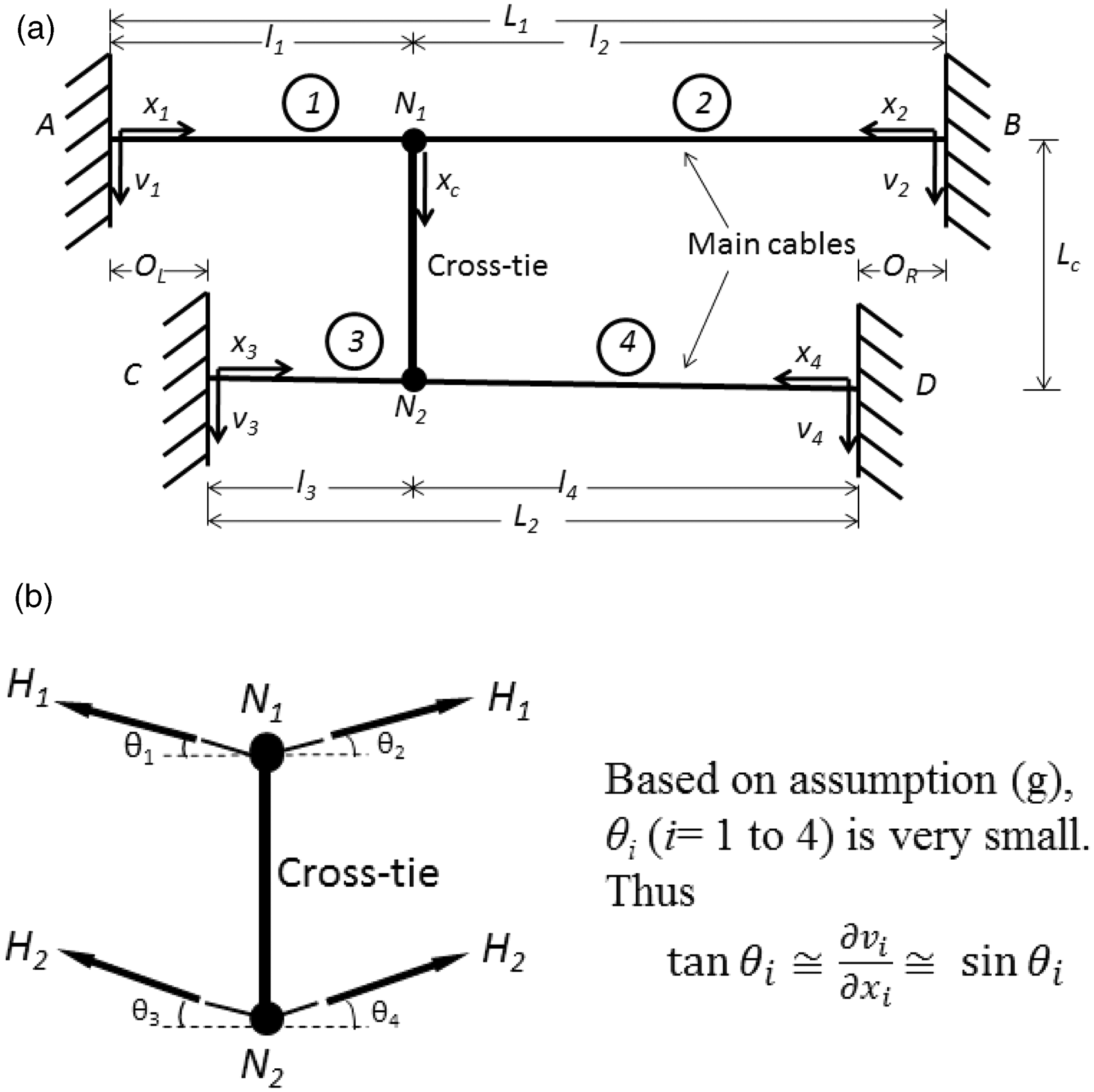

The analytical model of a basic cable network is developed based on the following assumptions: (a) the main cables are idealized as taut cables; (b) the additional dynamic tensions in the main cables are neglected; (c) the main cables are fixed at both ends; (d) the main cables have the in-plane transverse vibration as their dominant motion, while the longitudinal vibration is neglected; (e) the cross-tie is rigid; (f) the motion of the cross-tie is dominated by longitudinal vibration, while the transverse motion is neglected; (g) the vibration amplitude is small and thus the cables behave linearly.

2.2. In-plane free vibration of a single taut cable

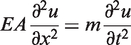
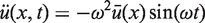
As can be seen from Figure 1(a), when the cable network vibrates in the vertical direction, the two main cables are expected to oscillate transversely, and that of the cross-tie along its axial direction. Therefore, the equation of motion describing the in-plane transverse vibration and axial vibration of a single taut cable will be briefly reviewed first.

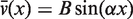
Since the additional cable tension due to its motion is neglected, the in-plane free vibration of a single taut cable in the transverse direction can be expressed as (Irvine and Caughey, 1974)

H \frac{\partial 2 v}{\partial x 2} = m \frac{\partial 2 v}{\partial t 2}

(1)

where v, H, and m are, respectively, the transverse displacement, tension, and mass per unit length of the taut cable; whereas that for the in-plane longitudinal motion is (Humar, 2002)

EA \frac{\partial 2 u}{\partial x 2} = m \frac{\partial 2 u}{\partial t 2}

(2)

where u and EA are the axial displacement and axial stiffness of the taut cable, respectively. By applying the Bernoulli–Fourier method to the in-plane transverse displacement

v (x, t)

to separate the time-dependent and spatial coordinate variables, it gives

v (x, t) = \bar{v} (x) \sin (ω t)

, where

\bar{v} (x)

is the shape function, and ω is the circular frequency of vibration. Its second derivative with respect to time t and spatial coordinate x are, respectively

\overset{··}{v} (x, t) = - ω 2 \bar{v} (x) \sin (ω t)

and

v ″ (x, t) = \bar{v} ″ (x) \sin (ω t)

Substitute the above two equations into Equation (1) and simplify it, giving

\bar{v} ″ (x) + α 2 \bar{v} (x) = 0

(3)

where

α = \sqrt{m ω 2 / H}

is the wave number. The solution to Equation (3) is in the form of

\bar{v} (x) = A \cos (α x) + B \sin (α x)

(4)

where A and B are constants, which can be determined from boundary conditions.

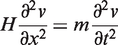
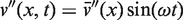
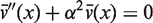
Since the cable is suspended horizontally and fixed at both ends, $\bar{v} (0) = 0 and \bar{v} (L) = 0$ . Applying these two boundary conditions to Equation (4) gives A = 0 and B $\sin (α L) = 0$ . The constant B cannot be zero in order for a nontrivial solution, thus

\bar{v} (x) = B \sin (α x)

(5)

Similarly, the in-plane axial displacement u

(x, t)

in Equation (2) can be expressed as

u (x, t) = \bar{u} (x) \sin (ω t)

by separating the variables, where

\bar{u} (x)

is the shape function. Its second derivative with respect to time t and spatial coordinate x are, respectively

\overset{··}{u} (x, t) = - ω 2 \bar{u} (x) \sin (ω t)

and

u ″ (x, t) = \bar{u} ″ (x) \sin (ω t)

Substitute the above two equations into Equation (2), yielding

\bar{u} ″ (x) + β 2 \bar{u} (x) = 0

(6)

where

β = \sqrt{m ω 2 / (EA)}

is the wave number. The solution to Equation (6) is in the form of

\bar{u} (x) = C \cos (β x) + D \sin (β x)

(7)

where C and D are constants determined from boundary conditions.

2.3. Formulation of the system equation

In the basic cable network model shown in Figure 1(a), there are four main cable segments vibrating in the transverse direction and one cross-tie in the axial direction. Equations (5) and (7) can thus be applied to describe their motions. By introducing the frequency ratio parameters $η_{i} = f_{1} / f_{i}$ and $η_{c} = f_{1} / f_{c}$ , and the nondimensional system frequency Ω = $π f / f_{1}$ , where $f_{i}$ and $f_{c}$ are the fundamental frequency of the ith (i = 1, 2) cable and the cross-tie, respectively, and f is the fundamental frequency of the cable network yet to be determined, the wave numbers $α$ and $β$ in Equations (5) and (7) can be expressed as $α_{i} = Ω η_{i} / L_{i}$ (i = 1, 2) and $β = Ω η_{c} / L_{c}$ . Thus, Equations (5) and (7) can be rewritten as

{\bar{v}}_{2 i - 1} (x_{2 i - 1}) = B_{2 i - 1} \sin (Ω η_{i} x_{2 i - 1} / L_{i}) i = 1, 2

(8a)

{\bar{v}}_{2 i} (x_{2 i}) = B_{2 i} \sin (Ω η_{i} x_{2 i} / L_{i}) i = 1, 2

(8b)

{\bar{u}}_{c} (x_{c}) = C \cos (Ω η_{c} x_{c} / L_{c}) + D \sin (Ω η_{c} x_{c} / L_{c})

(8c)

where i is the numbering of the main cables,

B_{2 i - 1}

and

B_{2 i}

are the shape function constants of the four main cable segments shown in Figure 1(a), and C, D are the shape function constants of the cross-tie. It is worth noting that based on the definition, the frequency ratio η₁ of the target cable (main cable 1) is 1. Equations (8a) and (8b) represent, respectively, the response of the left and the right segments of the two main cables in Figure 1(a), whereas Equation (8c) is for the cross-tie. The six unknown shape function constants B₁, B₂, B₃, B₄, C, and D can be determined using the following conditions.

Compatibility conditions

{\bar{v}}_{1} (l_{1}) = {\bar{v}}_{2} (l_{2}); {\bar{v}}_{3} (l_{3}) = {\bar{v}}_{4} (l_{4});

(9a)

{\bar{v}}_{1} (l_{1}) = {\bar{v}}_{3} (l_{3})

(9b)

{\bar{v}}_{1} (l_{1}) = {\bar{u}}_{1} (0)

(9c)

{\bar{u}}_{1} (0) = {\bar{u}}_{1} (L_{c})

(9d)

Equilibrium conditions

As shown in Figure 1(b), by isolating the cross-tie N₁N₂ from the network, forces acting on it should satisfy

H_{1} (\frac{\partial {\bar{v}}_{1}}{\partial x_{1}} |_{x_{1} = l_{1}} + \frac{\partial {\bar{v}}_{2}}{\partial x_{2}} |_{x_{2} = l_{2}}) + H_{2} (\frac{\partial {\bar{v}}_{3}}{\partial x_{3}} |_{x_{3} = l_{3}} + \frac{\partial {\bar{v}}_{4}}{\partial x_{4}} |_{x_{4} = l_{4}}) = 0

(9e)

Applying the above compatibility and equilibrium conditions to Equation (8) and expressing the resulting equations in the matrix form yields

[\sin (Ø_{1}) - \sin (Ø_{2}) 000000 \sin (Ø_{3}) - \sin (Ø_{4}) 00 \sin (Ø_{1}) 0 - \sin (Ø_{3}) 000 \sin (Ø_{1}) 000 - 1 00000 1 - \cos (Ø_{c}) \sin (Ø_{c}) γ_{1} \cos (Ø_{1}) γ_{1} \cos (Ø_{2}) γ_{2} \cos (Ø_{3}) γ_{2} \cos (Ø_{4}) 00] [B_{1} B_{2} B_{3} B_{4} C D] = [000000]

(10)

where $Ø_{2 i - 1} = Ω η_{i} ɛ_{2 i - 1}$ (i = 1, 2) applies to the left segments of both main cables with $ɛ_{2 i - 1} = l_{2 i - 1} / L_{i}$ being their segment ratios; $Ø_{2 i} = Ω η_{i} ɛ_{2 i}$ (i = 1, 2) applies to the right segments of both main cables with the corresponding segment ratios as $ɛ_{2 i} = l_{2 i} / L_{i}$ ; $Ø_{c} = Ω η_{c}$ applies to the cross-tie and $γ_{i} = \sqrt{H_{i} m_{i} / (H_{1} m_{1})}$ (i = 1, 2) is the mass-tension ratio parameter of the ith cable. It is worth mentioning that similar nondimensional parameters as the frequency ratio and the mass-tension ratio were used by Caracoglia and Jones (2005b) in deriving an analytical model for a perfectly orthogonal multi-stay multi-cross-tie network. To obtain the nontrivial solution to Equation (10), the determinant of the 6 × 6 coefficient matrix on the left-hand side of the equation should be zero, that is

| \sin (Ø_{1}) - \sin (Ø_{2}) 000000 \sin (Ø_{3}) - \sin (Ø_{4}) 00 \sin (Ø_{1}) 0 - \sin (Ø_{3}) 000 \sin (Ø_{1}) 000 - 1 00000 1 - \cos (Ø_{c}) \sin (Ø_{c}) γ_{1} \cos (Ø_{1}) γ_{1} \cos (Ø_{2}) γ_{2} \cos (Ø_{3}) γ_{2} \cos (Ø_{4}) 00 | = 0

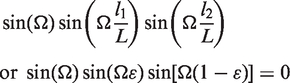
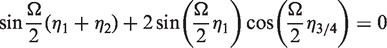
This leads to

γ_{1} \sin (Ø_{1}) \cos (Ø_{2}) sin (Ø_{3}) sin (Ø_{4}) sin (Ø_{c}) + γ_{1} \cos (Ø_{1}) \sin (Ø_{2}) sin (Ø_{3}) sin (Ø_{4}) sin (Ø_{c}) + γ_{2} \sin (Ø_{1}) \sin (Ø_{2}) sin (Ø_{3}) cos (Ø_{4}) sin (Ø_{c}) + γ_{2} \sin (Ø_{1}) \sin (Ø_{2}) cos (Ø_{3}) sin (Ø_{4}) sin (Ø_{c}) = 0

After trigonometric simplifications, it yields

\sin (Ω η_{c}) [γ_{1} \sin (Ω η_{1}) \sin (Ø_{3}) \sin (Ø_{4}) + γ_{2} \sin (Ω η_{2}) \sin (Ø_{1}) \sin (Ø_{2})] = 0

(11)

This equation is the system equation of a basic cable network where two horizontally suspended taut cables are connected transversely through a rigid cross-tie. It has two sets of solutions. The first set, which can be determined from sin(

Ω η_{c}

) = 0, represents the behavior of the cross-tie. It is of no interest to the present study and therefore is dropped. The second set of solutions can be obtained from

γ_{1} \sin (Ω η_{1}) \sin (Ø_{3}) \sin (Ø_{4}) + γ_{2} \sin (Ω η_{2}) \sin (Ø_{1}) \sin (Ø_{2}) = 0

(12)

which is the characteristic equation of the basic cable network in Figure 1. It can be observed from Equation (12) that the left-hand side of the equation is the summation of two terms. Each term is the product of four sub-terms, which are the mass-tension ratio parameter of one of the main cables, the Sine term of that main cable, and the Sine terms of both segments of the other main cable, respectively.

3. In-plane free vibration of a general cable network

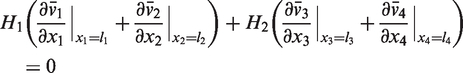
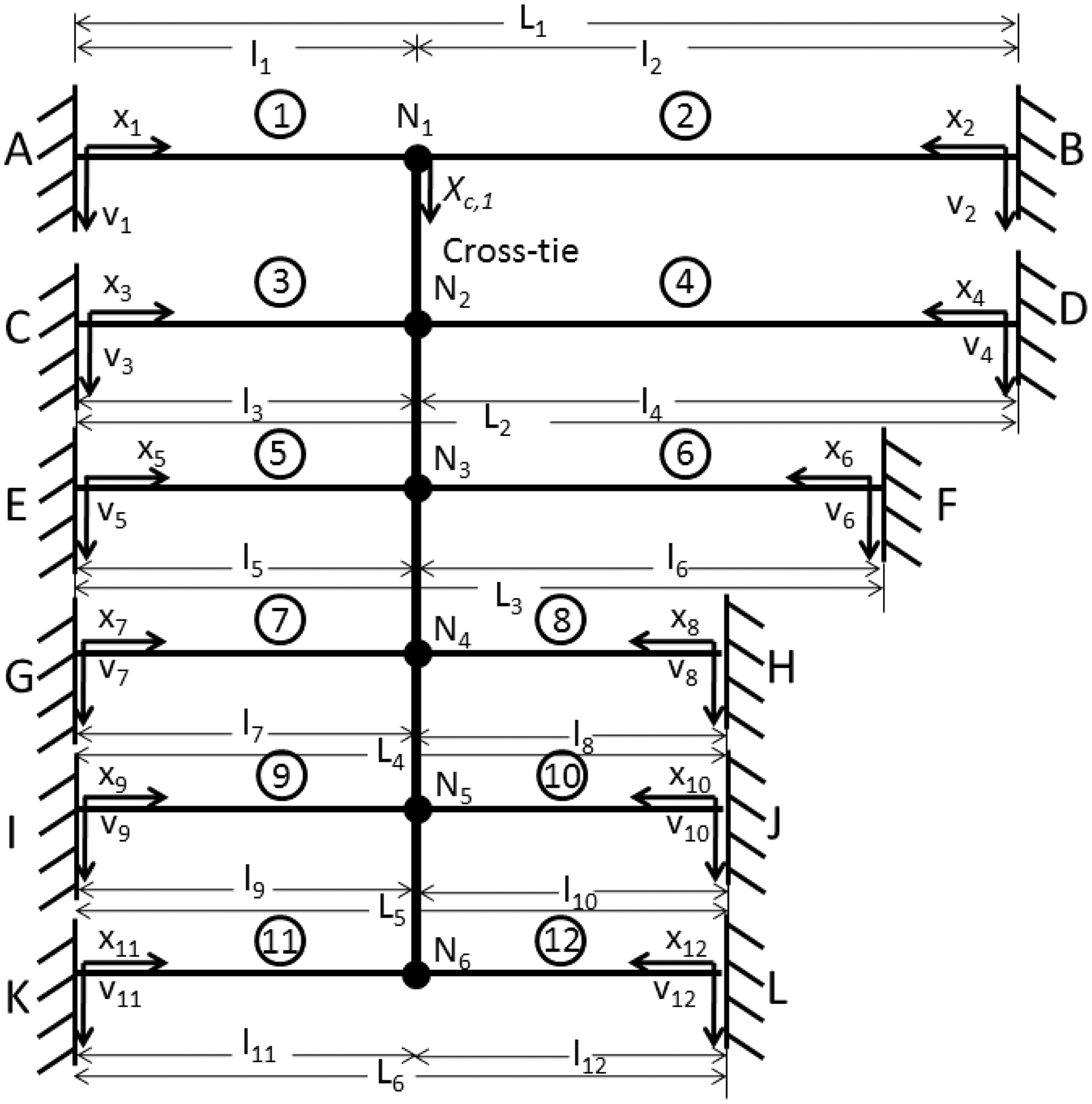
Before formulating the system equation of a general cable network, an extended cable network with four horizontally laid main cables will be studied first. As portrayed in Figure 2 (set n = 4 in the figure), this extended model comprises of four main cables of different lengths, with L₁ being the length of the longest cable, main cable 1 (target cable), in the network. To control vibrations of the target cable, it is connected to three other neighboring cables through a single line of transverse rigid cross-ties of lengths L_c_,_i (i = 1, 2, 3), which divide each main cable into two segments. They are labeled as shown in Figure 2. Assume the mass per unit length of cable i is m_i and the prestressing force is H_i (i = 1–4). The position of the cross-tie is l₁ from the left support of main cable 1. By applying the same assumptions and procedures described in Section 2 for a basic cable network, the characteristic equation of an extended cable network can be derived. The following boundary, compatibility, and equilibrium conditions are applied to this extended cable network model in the derivation.

Figure 2.

Schematic diagram of the mathematical model of a general cable network.

Boundary conditions

{\bar{v}}_{2 i - 1} (0) = 0, {\bar{v}}_{2 i} (0) = 0 i = 1, 2, 3, 4

(13a)

Compatibility conditions

{\bar{v}}_{2 i - 1} (l_{2 i - 1}) = {\bar{v}}_{2 i} (l_{2 i}) i = 1, 2, 3, 4

(13b)

{\bar{v}}_{2 i - 1} (l_{2 i - 1}) = {\bar{v}}_{2 i - 3} (l_{2 i - 3}) i = 2, 3, 4

(13c)

Equilibrium conditions

\sum_{i = 1}^{4} (\frac{\partial {\bar{v}}_{2 i - 1}}{\partial x_{2 i - 1}} |_{x_{2 i - 1} = l_{2 i - 1}} + \frac{\partial {\bar{v}}_{2 i}}{\partial x_{2 i}} |_{x_{2 i} = l_{2 i}}) H_{i} = 0

(13d)

Equation (13d) represents the longitudinal equilibrium of the single line of cross-ties by isolating them from the network. The summation of the transverse components of the main cable tension due to vibration should be zero at any arbitrary time instant t.

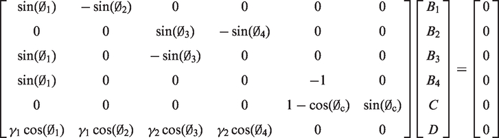
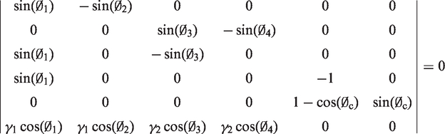
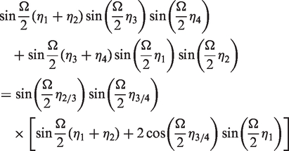
As a result, the system characteristic equation of an extended cable network is derived to be

γ_{1} \sin (Ω η_{1}) \sin (Ø_{3}) \sin (Ø_{4}) \sin (Ø_{5}) \sin (Ø_{6}) \sin (Ø_{7}) \sin (Ø_{8}) + γ_{2} \sin (Ω η_{2}) \sin (Ø_{1}) \sin (Ø_{2}) \sin (Ø_{5}) \sin (Ø_{6}) \sin (Ø_{7}) \sin (Ø_{8}) + γ_{3} \sin (Ω η_{3}) \sin (Ø_{1}) \sin (Ø_{2}) \sin (Ø_{3}) \sin (Ø_{4}) \sin (Ø_{7}) \sin (Ø_{8}) + γ_{4} \sin (Ω η_{4}) \sin (Ø_{1}) \sin (Ø_{2}) \sin (Ø_{3}) \sin (Ø_{4}) \times \sin (Ø_{5}) \sin (Ø_{6}) = 0

(14)

where Ω =

π f / f_{1}

is the nondimensional system frequency, f is the fundamental frequency of the cable network,

η_{i} = f_{1} / f_{i}

and

γ_{i} = \sqrt{H_{i} m_{i} / H_{1} m_{1}}

are, respectively, the frequency ratio and the mass-tension ratio parameter of the ith main cable,

f_{i}

m_{i}, H_{i}

are, respectively, the fundamental frequency, the unit mass, and the pretension of the ith cable in the network (i = 1–4), and

Ø_{2 i - 1} = Ω η_{i} ɛ_{2 i - 1}

and

Ø_{2 i} = Ω η_{i} ɛ_{2 i}

apply, respectively, to the left and the right segment of each main cable, with

ɛ_{2 i - 1} = l_{2 i - 1} / L_{i}

and

ɛ_{2 i} = l_{2 i} / L_{i}

being the segment ratio of the left and the right segment of the ith main cable (i = 1–4), respectively. Similar nondimensional parameters, such as the frequency ratio, the segment ratio, and the mass-tension ratio, were also defined by Caracoglia and Jones (2005b).

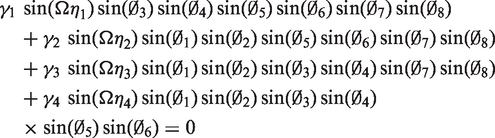
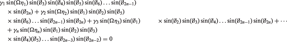
As can be seen from Equation (14), there are four main terms and each corresponds to one main cable in the network. Every term is the product of the mass-tension ratio parameter of one main cable, the combined Sine term of that main cable, and the Sine terms of both segments of the remaining three main cables. It shows the same pattern as Equation (12), which is the system characteristic equation of a basic cable network. Based on this observation, the characteristic equation of a more general cable network consisting of n (n = 2, 3, 4, … , N) horizontally laid main cables and a single line of rigid cross-ties, as shown in Figure 2, can be expressed as

γ_{1} \sin (Ω η_{1}) \sin (Ø_{3}) \sin (Ø_{4}) \sin (Ø_{5}) \sin (Ø_{6}) \dots \sin (Ø_{2 n - 1}) \times \sin (Ø_{2 n}) + γ_{2} \sin (Ω η_{2}) \sin (Ø_{1}) \sin (Ø_{2}) \sin (Ø_{5}) \times \sin (Ø_{6}) \dots \sin (Ø_{2 n - 1}) \sin (Ø_{2 n}) + γ_{3} \sin (Ω η_{3}) \sin (Ø_{1}) \times \sin (Ø_{2}) \sin (Ø_{3}) \sin (Ø_{4}) \dots \sin (Ø_{2 n - 1}) \sin (Ø_{2 n}) + \dots + γ_{n} \sin (Ω η_{n}) \sin (Ø_{1}) \sin (Ø_{2}) \sin (Ø_{3}) \times \sin (Ø_{4}) (Ø_{5}) \dots \sin (Ø_{2 n - 3}) \sin (Ø_{2 n - 2}) = 0

(15)

where n (n = 2, 3, 4 , … , N) is the number of main cables in the cable network.

From the above system characteristic equation and also noticing the definition of $Ø_{j}$ ( j = 1, 2, … , 2n), it can be clearly seen that the segment ratio $ɛ$ , the frequency ratio $η$ , the mass-tension ratio $γ$ , and the number of main cables n in the network are the four key system parameters that govern the in-plane modal behavior of a cable network with a single line of transverse rigid cross-ties.

4. Finite element model

To verify the proposed analytical model for the in-plane free vibration of a general cable network, a finite element model is developed independently. The commercial finite element software package ABAQUS 6.9 is used for this purpose. This software is capable of numerically simulating the performance of structural members in static, free vibration, and linear and nonlinear dynamic analysis.

In the developed model, all main cables and cross-ties are modeled as two-dimensional elements with two degrees-of-freedom along the transverse and axial directions at each node. The beam element B21 from the ABAQUS element library is chosen to model the main cable. This element is a shear-deformable (Timoshenko) beam and can be used for thin or thick members. The rigid beam element RB2D2 is selected to simulate the behavior of the rigid cross-ties. All the cables used in the numerical examples of the current study have lengths varying between 48 and 100 m. From the sensitivity analysis, it is concluded that 50–100 elements per cable, depending on the cable length, is adequate to model the cable behavior.

In order to ensure the accuracy of the results, the material properties of the numerical model must be defined to be compatible with the assumptions made for the analytical model. In the analytical model, the main cables are idealized as taut strings. Therefore, the material properties of the main cables in the finite element model are selected in such a way that would yield the Irvin’s inextensibility parameter close to 0. This parameter was introduced by Irvine and Caughey (1974) to describe the static and dynamic behavior of cables. It accounts for the geometric and elastic effects and is defined as λ²= (mgL/H)²L/[HL_e/(EA)], where L_e is the effective length of the cable due to the sagging effect. The value of λ² varies from a very small number (close to 0), for the taut flat cable, to a very large number (for example, 1000) in the case of an inextensible cable. The cross-ties are idealized as rigid connectors in the analytical model. Therefore, it is taken as the rigid body in the finite element model. The main cables are fixed at both ends and the initial stress is introduced to the B21 elements to simulate the effect of pretension. All boundary conditions are defined when building the finite element model, and the initial stress in the B21 elements is applied as the initial condition.

For free vibration analysis, the FREQUENCY procedure in the ABAQUS software is adopted, which uses an eigenvalue technique to extract natural frequencies and the corresponding mode shapes of a structure. LANCZOS is used as the Eigen solver. In the output, the eigenvectors are normalized such that the largest displacement value in each vector is unity.

5. Applications to cable networks with different configurations

In this section, the proposed analytical model of a general cable network will be applied to a number of cable network systems having different configurations and structural properties to demonstrate its flexibility. Results will be compared with those obtained from numerical simulations using the finite element model described in Section 4. The unique modal behavior associated with different types of cable network will be discussed.

5.1. Twin-cable network

5.1.1. Cross-tie at arbitrary location

In this type of cable network configuration, the two main cables are twins, that is, $L_{1} = L_{2} = L$ , $H_{1} = H_{2}$ , and $m_{1}$ = $m_{2}$ . Assume the cross-tie locates at a distance l₁, with l₁ ≠ l₂, from the left end of main cable 1, as shown in Figure 3. Therefore, the frequency ratios are $η_{1} = η_{2} = 1,$ the mass-tension ratios are $γ_{1} = γ_{2} = 1$ , and the segment ratios are $ɛ_{1} = ɛ_{3} = l_{1} / L = ɛ$ and $ɛ_{2} = ɛ_{4} = l_{2} / L = 1 - ɛ$ . Because the mass-tension ratio parameter γ is the same for both cables, it is termed as the same-mass-tension ratio or SMT cable network. Substitute these values into Equation (12), giving

\sin (Ω) \sin (Ω \frac{l_{1}}{L}) \sin (Ω \frac{l_{2}}{L}) or \sin (Ω) \sin (Ω ɛ) \sin [Ω (1 - ɛ)] = 0

(16)

Obviously, three sets of solution are present for Equation (16). The first set, yielded from

\sin (Ω) = 0

, generates roots of Ω = nπ, where n = 1, 2, 3 … . It describes the global modes of the entire cable network system, of which the two main cables vibrate at the same natural frequency of a single cable. The odd values of n generate the system frequencies of

Ω = π, 3 π, 5 π \dots

for the symmetric modes, whereas the even values of n generate the system frequencies of

Ω = 2 π, 4 π, 6 π \dots

for the anti-symmetric modes. Clearly, the expression of the system frequency associated with the global modes, that is,

Ω = n π

, is not a function of the segment ratio

ɛ

. This suggests that if the cross-tie is rigid, both the symmetric and the anti-symmetric global modes of a twin SMT cable network are independent of the position of the cross-tie. In these global modes, both main cables vibrate in the same shape as that of a single cable at this frequency.

Figure 3.

Schematic diagram of a symmetric twin-cable network with rigid cross-tie at an arbitrary point.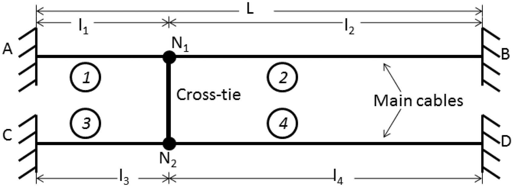

The second and the third sets of solution are functions of the segment ratio $ɛ$ , that is, the cross-tie position. They have the form of

Ω = n π / ɛ

(17a)

and

Ω = n π / (1 - ɛ)

(17b)

where n = 1, 2, 3 … . The modal frequencies given by Equation (17a) result from the vibrations of cable segment 1 in main cable 1 and its counterpart in main cable 2, that is, segment 3, while the other two main cable segments are at rest. Similarly, vibrations of cable segments 2 and 4 in Figure 3 are associated with the frequencies given by Equation (17b). In this study, these two types of local modes are categorized as the left-segment mode (when the left segments are vibrating and the right ones are at rest, designated as ‘LS’ mode) and the right-segment mode (when the right segments are vibrating and the left ones are at rest, designated as ‘RS’ mode). For cross-tie position other than the mid-span, that is,

ɛ \neq 1 / 2

, it can be seen that the frequencies of the lower order modes of one equation in Equation (17) may be the same as those of the higher order ones of the other equation, that is, they form complimentary pairs. Caracoglia and Jones (2005a) denoted these ‘LS’ and ‘RS’ modes as the ‘complimentary-pseudo-symmetric’ and the ‘pseudo-symmetric’ modes. For cross-tie position at the mid-span, frequencies and mode shapes of the LS modes are the same as those of the RS modes.

The impact of the cross-tie position, that is, the segment ratio $ɛ$ , on the system frequency of a twin-cable network with a transverse rigid cross-tie is illustrated in Figure 4. As can be observed from the figure, while the frequencies of the global modes, which are independent of the cross-tie position, remain as constants nπ (n = 1, 2, 3 … ) as the cross-tie moves from the left end of the main cables towards right, the frequencies of the local LS modes gradually decrease and those of the local RS modes increase. The frequency variation of the local LS modes and RS modes are symmetric about the center line of $ɛ = 1 / 2$ and complimentary with each other. At certain cross-tie positions, more than one global or local modes have the same modal frequency. Thus, the Ω- $ɛ$ curve of these modes will intersect with each other at those locations. Three types of intersections can be observed from Figure 4.

Figure 4.

Nondimensional modified frequency, 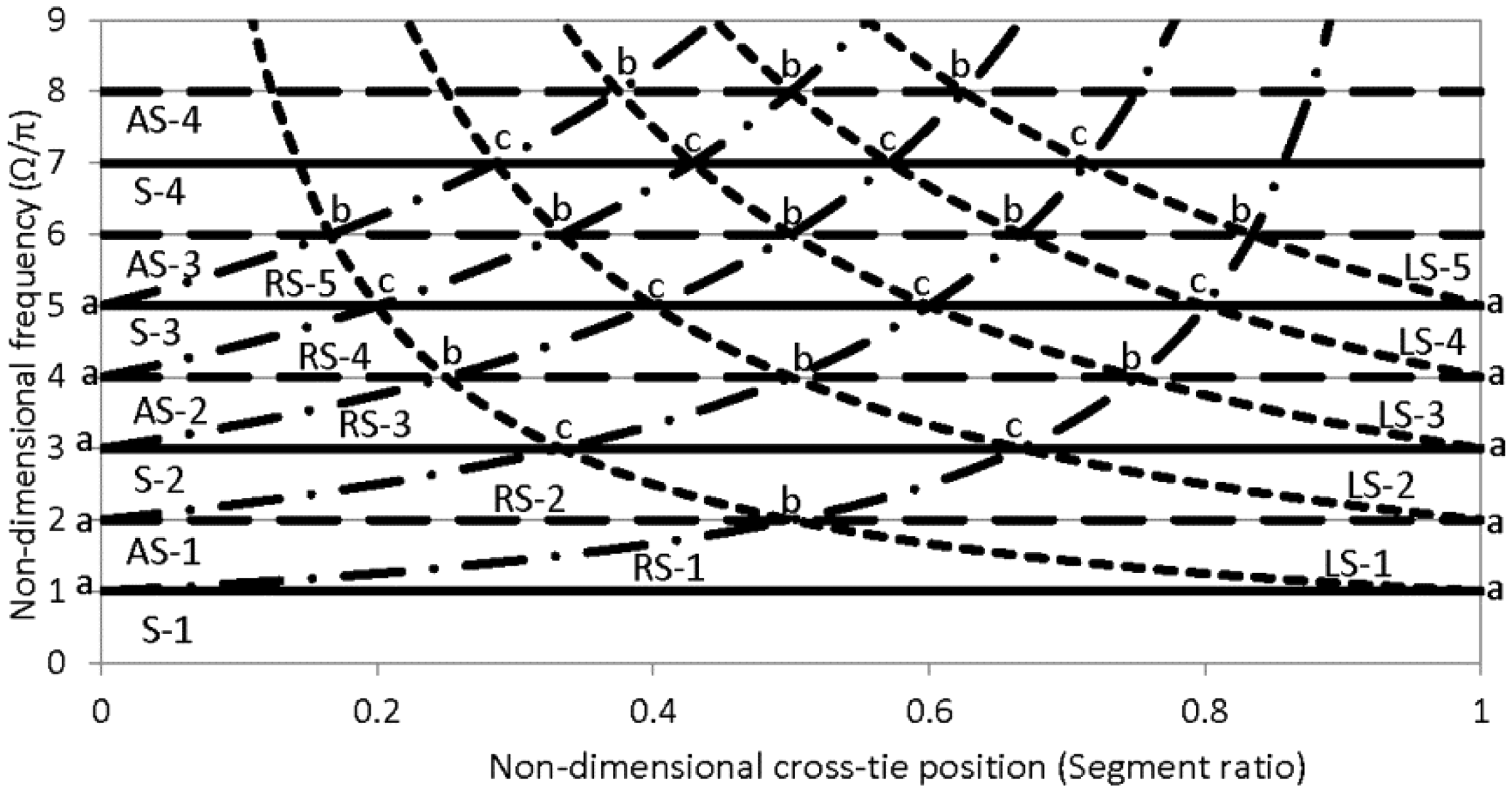$Ω$ / $π$ , as a function of the nondimensional cross-tie position, $ɛ$ , for a twin-cable same-mass-tension (SMT) network (global symmetric, solid line), AS (global asymmetric, broken line), RS (local, right segment, dash-dot line), and LS (local, left segment, dotted line) modes.

The first type of intersection, symbolized by ‘a’, represents the extreme cases of cross-tie location either at the left ( $ɛ = 0)$ or the right ( $ɛ = 1)$ support of the main cables. When $ɛ = 0$ , the lengths of the main cable left segments are zero. Thus, the local RS modes are the same as the global modes. Similarly, the lengths of the right cable segments become zero when $ɛ = 1$ , and the local LS modes are the same as the global ones.

The second type of intersection, denoted by ‘b’, represents the coexistence of a pair of complimentary local RS mode and LS mode, along with an asymmetric global mode. The corresponding cross-tie position can be found by equating the frequency of the asymmetric global mode with one of the local modes in the complimentary pair. Using the case of the second asymmetric global mode as an example, its frequency remains as a constant when $ɛ$ increases from 0 to 1, which is shown in Figure 4 as a horizontal broken line Ω = 4π. There are three Type II intersection points on this horizontal line. The one on the left represents the coexistence of the first LS mode, the third RS mode, and the second asymmetric global mode. The frequency of the first LS mode can be computed from Equation (17a) by substituting n = 1, which gives Ω = π/ $ɛ$ . By equating it with the frequency of the second asymmetric global mode, it yields π/ $ɛ = 4 π$ , based on which the location of the cross-tie can be determined as $ɛ = 1 / 4$ . Similarly, the cross-tie locations corresponding to the other two intersection points ‘b’ are found to be $ɛ = 1 / 2$ and $ɛ = 3 / 4$ , respectively.

The third type of intersection is symbolized by ‘c’; it is associated with the coexistence of a complimentary pair of local RS and LS modes and a symmetric global mode. The cross-tie location where these three modes coexist can be determined similarly by equating the frequency of the symmetric global mode with one of the local modes in the complimentary pair. For example, for the two intersection points ‘c’ on the horizontal solid line of Ω = 3π, the corresponding cross-tie positions are $ɛ = 1 / 3$ and $ɛ = 2 / 3$ , respectively.

It is interesting to note that the cross-tie position corresponding to the second and the third types of intersections happens to be the common node shared by the mode shapes of all the coexisted modes. In addition, results in Figure 4 clearly indicate that because of the modal property tri-furcation at the intersection points ‘b’ and ‘c’, the modal behavior of such a twin-cable network is very sensitive in the vicinity of these intersections. A minor shift of the cross-tie position could lead to a drastic switch between a local mode and a global mode, or a local LS mode and its complimentary RS mode. An earlier study by Caracoglia and Jones (2005a) also reported the coexistence of a pair of local modes and a global mode at some specific cross-tie locations. However, the intersection points were classified into two different types based on whether or not the cross-tie is located at cable mid-span.

5.1.2. Special case 1: cross-tie at mid-span

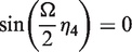
For a special case of cross-tie locates at the mid-span, all four main cable segments have the same segment ratio of $ɛ_{j} =$ 1/2 (j = 1–4) and, thus, $Ø_{j} =$ Ω/2 (j = 1–4). Substitute these values into Equation (12), giving

2 \sin (Ω) \sin (\frac{Ω}{2}) \sin (\frac{Ω}{2}) = 0 .

(18)

It is worth pointing out that when studying the same type of twin-cable network, Caracoglia and Jones (2005a) derived a system characteristic polynomial (Equation (9) in the reference), which, by setting it as zero, would give the modal frequencies of a twin-cable network with a rigid cross-tie placed at the mid-span. This characteristic polynomial, although looks slightly different in form, is actually the same as Equation (18) derived independently above.

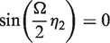
Among the three sets of solution to Equation (18), the one that describes the global modes, which yielded from $\sin (Ω) = 0$ , is not affected by the cross-tie position. The other two sets, both derived from the condition of $\sin (Ω / 2) = 0$ , are the same in terms of the magnitude of the modal frequency. However, the associated mode shapes corresponding to these two sets are totally different. The second set condition originates from $\sin (Ø_{1}) = \sin (Ω / 2) = 0$ . It generates the system frequency of $Ω = 2 n π (n = 1, 2, 3 \dots)$ . These are the same as the frequencies of the anti-symmetric global modes given by the first set. The corresponding mode shapes are the local LS modes, which are dominated by the vibrations of the left cable segments. On the other hand, the third set condition, which is $\sin (Ø_{2}) =$ $\sin (Ω / 2) = 0$ , although it gives the same system frequencies as those from the second set, represents the local RS modes of which only the right cable segments are in motion.

The mode shapes, that is, the vectors of the normalized modal amplitudes, can be determined by substituting the frequency values into Equation (10). The odd values of n generate symmetric global modes, that is, [1 1 1 1]^T, while the even values of n generate three different possible vectors of normalized modal amplitudes as explained above, that is:

[1 −1 1 −1]^T: anti-symmetric global modes with in-phase motion of both cables;

[0 −1 0 1]^T: local RS modes with out-of-phase motion of right cable segments;

[1 0 −1 0]^T: local LS modes with out-of-phase motion of left cable segments.

The left half of Figure 5 presents the first four modes of this type of basic cable network, the mode shape of which are defined by the above four normalized modal amplitude vectors.

Figure 5.

Typical modes of a symmetric twin-cable system with rigid cross-tie at mid-span and quarter span (GM: global mode; LM: local mode; Sym.: symmetric; Asym.: anti-symmetric; RS: right segment; LS: left segment).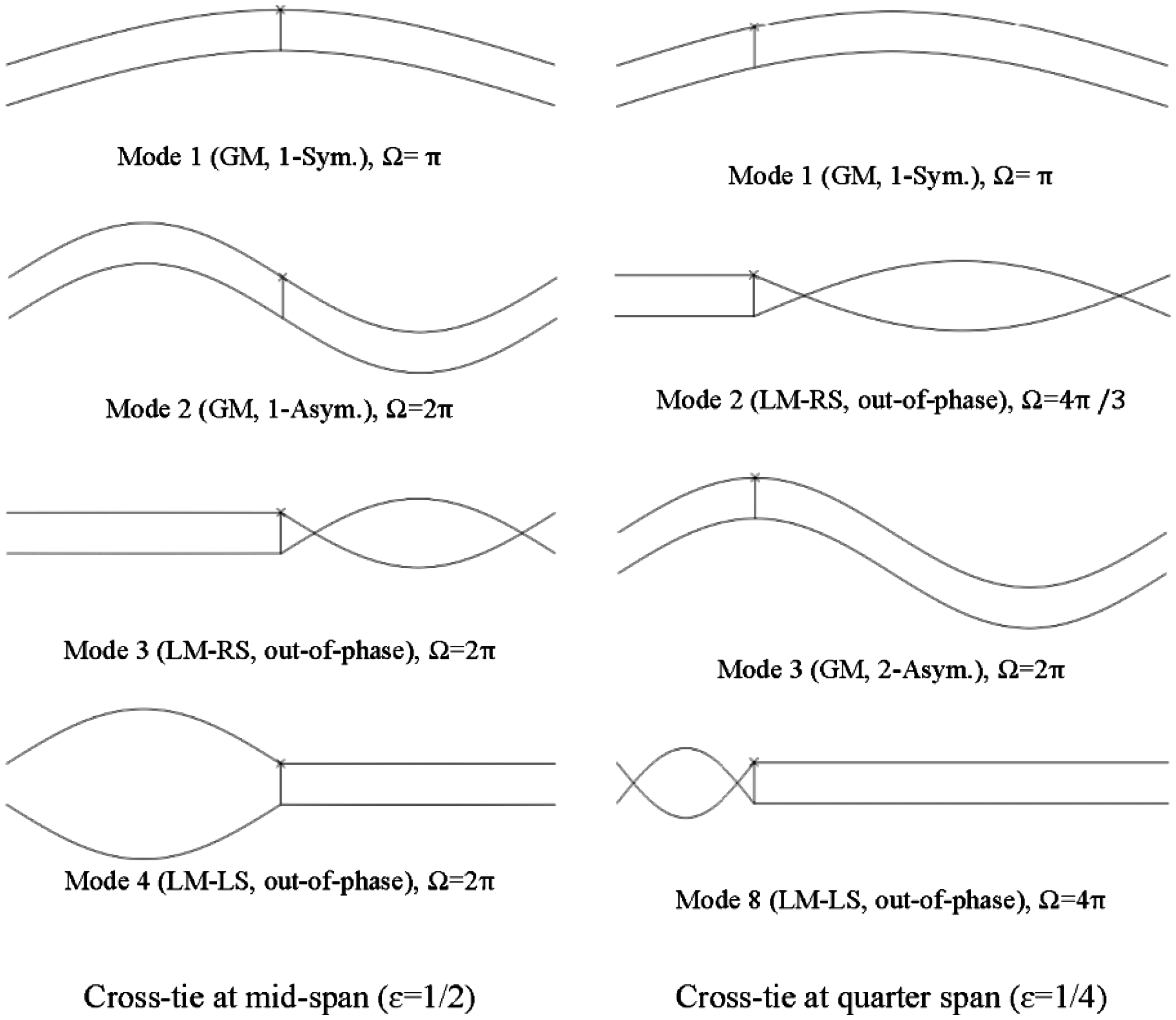

5.1.3. Special case 2: cross-tie at quarter span

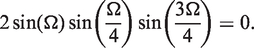
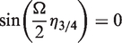
Similarly, when the cross-tie locates at the quarter span from the left support, Equation (12) becomes

2 \sin (Ω) \sin (\frac{Ω}{4}) \sin (\frac{3 Ω}{4}) = 0 .

(19)

Again, three sets of solution are available. By comparing with the case of rigid cross-tie locates at the mid-span, it can be clearly observed that the global modes, derived from

\sin (Ω) = 0

, are the same. However, by varying the segment ratio from ɛ = 1/2 to ɛ = 1/4, the lengths of the right segments, segments 2 and 4 in Figure 3, are increased, whereas those of the left segments, segments 1 and 3, are reduced. Consequently, the local RS modes, yielded from

\sin (3 Ω / 4) = 0

, appear early with lower frequencies, whereas the local LS modes, described by

\sin (Ω / 4) = 0

, are delayed due to its increased frequencies. The above fact suggests that the modal order of a twin-cable network would be affected by the cross-tie position.

5.1.4. Numerical examples

To validate the proposed analytical model and the derived modal solutions of a twin-cable network, two numerical examples are presented in this section. The twin main cables in both examples are assumed to be the same as the type AS14 cable on the Fred Hartman Bridge (Caracoglia and Jones, 2005b), that is, both having a pretension of 1598 kN, a unit mass of 47.9 kg/m, and a length of 67.34 m. Two cross-tie locations of ɛ = 1/2 and ɛ = 1/4 are considered. The natural frequencies and the mode shapes of the first 10 modes of these two-cable networks are listed in Table 1. A comparison between the two sets of modal analysis results in the table show that by moving the cross-tie from mid-span to quarter span, although modal properties of the global modes remain the same, the modal order is altered. More local RS modes appear within the first 10 modes due to longer and thus more flexible right cable segments. The frequencies of the local RS modes become lower, which advances their modal order. Besides, the modal analysis results yielded from the finite element simulation in ABAQUS are also given in Table 1. They are found to agree well with the analytical ones, which verifies the validity of the proposed analytical model. Four selected typical modes corresponding to each of the two studied twin-cable networks are portrayed in Figure 5. They include the lowest symmetric and anti-symmetric global modes, and the lowest LS and RS modes.

Table 1.

In-plane modal properties of twin-cable networks with a rigid cross-tie at mid-span and quarter span.

Mode number	$ɛ$ = 1/2			$ɛ$ = 1/4
	Modal frequency (Hz)		Mode shape	Modal frequency (Hz)		Mode shape
	Analytical	FEA	Mode shape	Analytical	FEA	Mode shape
1	1.3562	1.3563	GM, 1-Sym., in-phase	1.3562	1.3563	GM, 1-Sym., in-phase
2	2.7124	2.7126	GM, 1- Asym., in-phase	1.8082	1.8084	LM-RS, out-of-phase
3	2.7124	2.7126	LM-RS, out-of-phase	2.7124	2.7123	GM, 1- Asym., in-phase
4	2.7124	2.7126	LM-LS, out-of-phase	3.6165	3.6161	LM-RS, out-of-phase
5	4.0685	4.0676	GM, 2-Sym., in-phase	4.0685	4.0678	GM, 2-Sym., in-phase
6	5.4247	5.4226	GM, 1- Asym., in-phase	5.4247	5.4221	LM-RS, out-of-phase
7	5.4247	5.4226	LM-RS, out-of-phase	5.4247	5.4226	GM, 1- Asym., in-phase
8	5.4247	5.4226	LM-LS, out-of-phase	5.4247	5.4240	LM-LS, out-of-phase
9	6.7809	6.7749	GM, 3-Sym., in-phase	6.7809	6.7753	GM, 3-Sym., in-phase
10	8.1371	8.1273	GM, 3- Asym., in-phase	7.2330	7.2259	LM-RS, out-of-phase

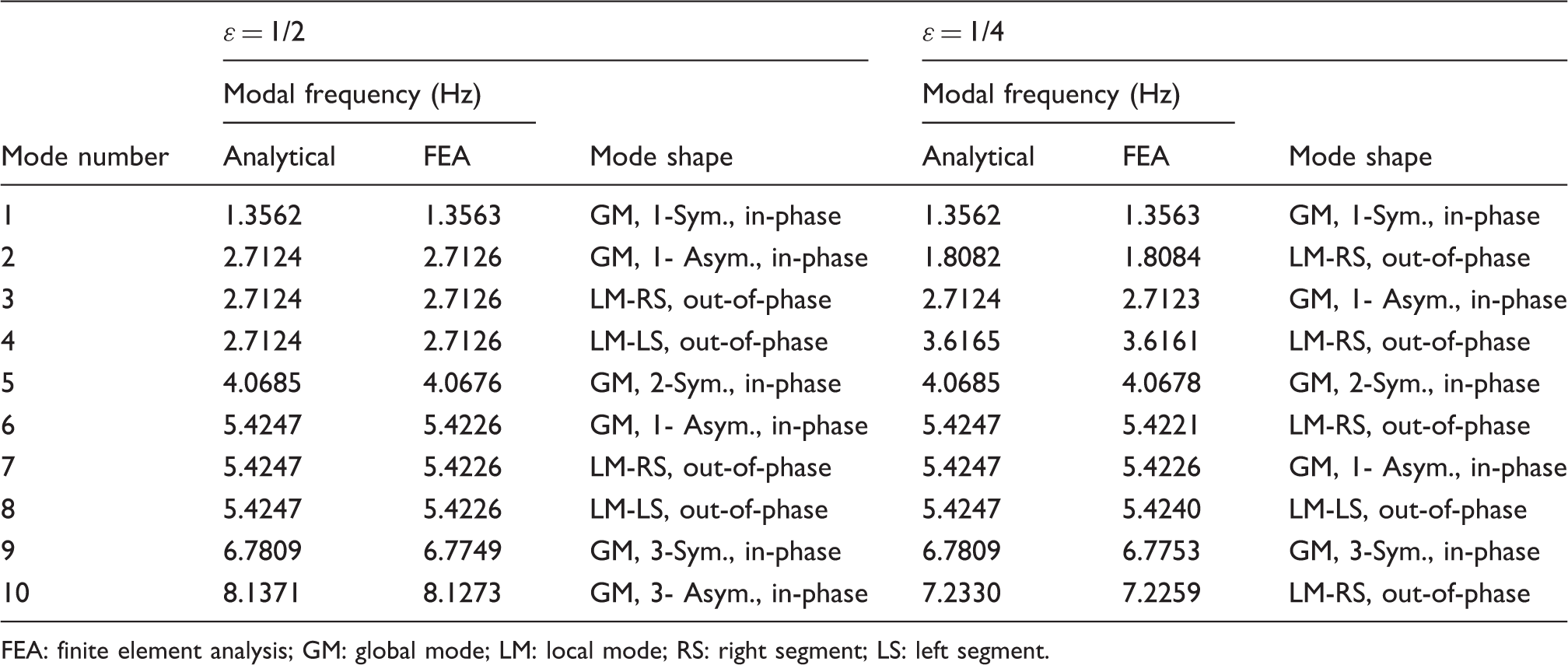
FEA: finite element analysis; GM: global mode; LM: local mode; RS: right segment; LS: left segment.

5.2. Symmetric unequal length two-cable network with a rigid cross-tie at mid-span

5.2.1. Analytical solution

In a symmetric two-cable network, shown in Figure 6, the cross-tie locates at mid-span. Assume the two main cables have different lengths and mass-tension ratios. Thus, the frequency ratios are $η_{1} = 1$ , $η_{2} = m_{2} L_{2} / m_{1} L_{1}$ ; the mass-tension ratios are $γ_{1} = 1$ but $γ_{1} \neq γ_{2}$ ; and the segment ratios for all segments are the same, that is, $ɛ_{j} =$ 1/2 (j = 1–4). Based on these, $Ø_{1} = Ø_{2} = Ω / 2$ and $Ø_{3} = Ø_{4} = Ω η_{2} / 2$ . Substitute these values into Equation (12), yielding

[\sin (\frac{Ω}{2} η_{2}) \cos (\frac{Ω}{2}) + γ_{2} \sin (\frac{Ω}{2}) \cos (\frac{Ω}{2} η_{2})] \times \sin (\frac{Ω}{2}) \sin (\frac{Ω}{2} η_{2}) = 0

(20)

Figure 6.

Symmetric same-mass-tension two-cable network with unequal length main cables and a rigid cross-tie at mid-span.

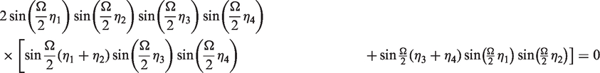
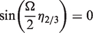
Three sets of solution are present for the above system characteristic equation, which can be derived from

\sin (\frac{Ω}{2} η_{2}) \cos (\frac{Ω}{2}) + γ_{2} \sin (\frac{Ω}{2}) \cos (\frac{Ω}{2} η_{2}) = 0

(21a)

\sin (\frac{Ω}{2}) = 0

(21b)

and

\sin (\frac{Ω}{2} η_{2}) = 0

(21c)

The condition described by Equation (21a) gives the global modes of the network, of which both main cables vibrate. As can be seen from the equation, the global modal frequencies are the functions of the frequency ratio parameter

η_{2}

as well as the mass-tension ratio parameter

γ_{2}

. This suggests that if a rigid cross-tie is used to connect a colleague cable to a target cable and placed at mid-span, the increment in the modal frequency of the target cable would be solely dependent on the mass, length, and pretension of the colleague cable.

As a special case, when the two main cables have the same mass-tension ratio, that is, $γ_{1} = γ_{2} = 1$ , the network in Figure 6 becomes a symmetric SMT cable network. Therefore, Equation (21a) can be reduced to

\sin [\frac{Ω}{2} (1 + η_{2})] = 0

(22)

which gives the nondimensional modal frequency of the network global modes as

Ω = 2 n π / (1 + η_{2})

(23)

The form of Equation (23) implies that in a symmetric SMT two-cable network, the frequency ratio,

η_{2} = f_{1} / f_{2}

, of the colleague cable would dictate the modal frequency of the system global modes. Such an impact on the fundamental frequency of the cable network is illustrated in Figure 7. The pattern of the curve suggests that in this type of cable network, if the lengths of the two main cables approach to be the same, the fundamental frequency of the network becomes lower. Once the lengths are equal, the fundamental system frequency would equal that of a single main cable. Thus, connecting a target cable to a colleague cable having the same mass-tension ratio and length using a rigid cross-tie will not help to increase its in-plane stiffness. This agrees with the finding in Section 5.1 for the twin-cable networks. In other words, in such a SMT network system, to further increase the in-plane stiffness of a target cable, it should be connected with a ‘colleague’ cable of shorter length, which itself is stiffer, and has a smaller value of frequency ratio

η_{2} .

Figure 7.

Nondimensional modified frequency, Ω/ $π$ , as a function of frequency ratio parameter, $η$ , for a symmetric same-mass-tension two-cable network.

Equations (21b) and (21c) generate the local modes dominated by either the target cable (main cable 1) or the colleague cable (main cable 2), respectively. As can be seen from Equations (21b) and (21c), the local modes dominated by the longer main cable (the target cable) are the same as those of the anti-symmetric modes of a single main cable, while those dominated by the shorter main cable (the colleague cable) depend on its frequency ratio. A stiffer colleague cable would lead to higher frequencies of its dominated local modes and delay its modal order.

5.2.2. Numerical examples

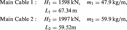
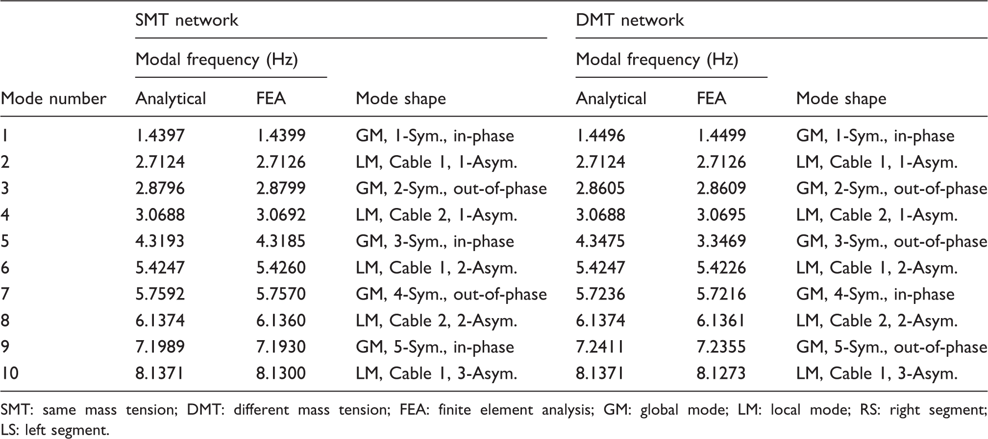
Two numerical examples of the symmetric unequal length two-cable network are presented in this section. To investigate the impact of the colleague cable on the modal behavior of the entire network, the same target cable is used in both examples. The colleague cable in Example 1 is assumed to have the same mass-tension ratio as the target cable, whereas that in Example 2 takes a different value. Thus, the cable network in Example 1 is a SMT system, and the one in Example 2 is a DMT system. The properties of the cables in these two networks are as follows.

Example 1 (SMT cable network)

Main Cable 1 : H_{1} = 1598 kN, m_{1} = 47.9 kg / m, L_{1} = 67.34 m Main Cable 2 : H_{2} = 1598 kN, m_{2} = 47.9 kg / m, L_{2} = 59.52 m

Example 2 (DMT cable network)

Main Cable 1 : H_{1} = 1598 kN, m_{1} = 47.9 kg / m, L_{1} = 67.34 m Main Cable 2 : H_{2} = 1997 kN, m_{2} = 59.9 kg / m, L_{2} = 59.52 m

Based on the above, the two-cable networks studied here have the same frequency ratios of η₁ = 1, η₂ = 0.88 and the same segment ratios of

ɛ_{j} =

1/2 ( j = 1–4). The mass-tension ratio parameter of the target cable is γ₁ = 1 in both cases, but that of the colleague cable increases from γ₂ = 1 in Example 1 to γ₂ = 1.25 in Example 2. The modal properties of the first 10 modes of both cable networks are listed in Table 2. In addition, the numerical simulation results obtained from ABAQUS are given in the same table, which are found to agree well with the analytical set. Compared to the SMT cable network in Example 1, the modal order and mode shapes of the lowest 10 modes in the corresponding DMT network remain unchanged. However, by connecting the same target cable (main cable 1) with its neighboring one having the higher mass-tension ratio parameter of γ₂ = 1.25, the fundamental frequency of the cable network is found to be slightly increased from 1.4397 Hz in Example 1 to 1.4496 Hz in Example 2. The analytical solution derived in Section 5.2.1 (Equation (23)) and the results of the numerical examples here suggest that to enhance the in-plane stiffness of a target cable, it should be connected with cable(s) either having the same or higher mass-tension ratio and/or lower frequency ratio. Since the target cables in both networks are the same, mode 2 in these two different cable networks, which is the local mode of main cable 1, has the same frequency and mode shape. In the case of main cable 2, however, although the one in Example 2 has higher pretension and unit mass as compared to its counterpart in Example 1, the frequency remains unchanged. Thus, mode 4 of both networks, which is the local mode dominated by main cable 2, has exactly the same modal properties. Figure 8 shows the first 10 mode shapes of the two studied networks. For each mode, the modal frequency of the SMT and the DMT system are given outside and inside the bracket, respectively.

Figure 8.

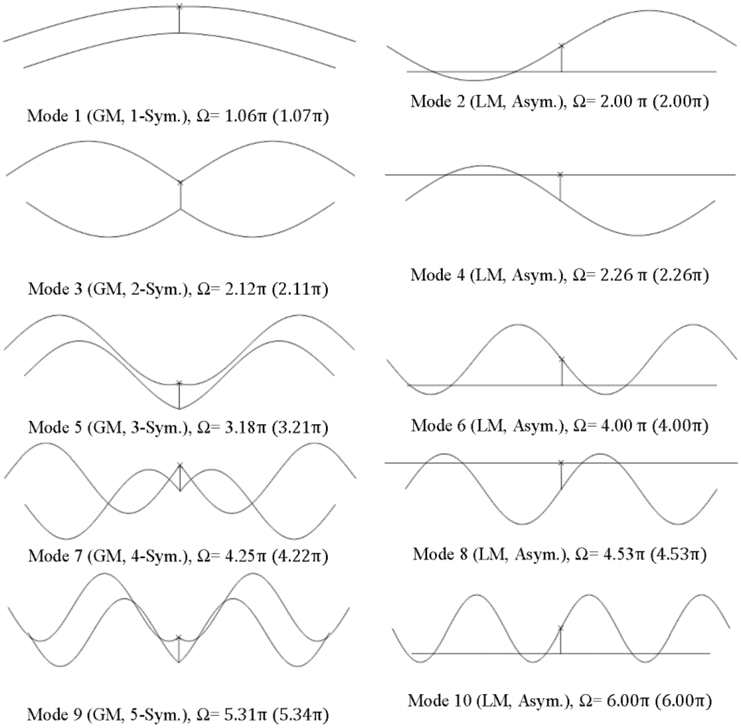
First 10 modes of a symmetric two-cable network with unequal length main cables and a rigid cross-tie at mid-span. (The abbreviated symbols used for describing the mode shapes are the same as those in Figure 5; in each mode, the modal frequencies corresponding to the same-mass-tension and the different-mass-tension networks are given outside and inside the brackets, respectively.)

Table 2.

In-plane modal properties of symmetric unequal length two-cable networks with a rigid cross-tie at mid-span.

Mode number	SMT network			DMT network
	Modal frequency (Hz)		Mode shape	Modal frequency (Hz)		Mode shape
	Analytical	FEA	Mode shape	Analytical	FEA	Mode shape
1	1.4397	1.4399	GM, 1-Sym., in-phase	1.4496	1.4499	GM, 1-Sym., in-phase
2	2.7124	2.7126	LM, Cable 1, 1-Asym.	2.7124	2.7126	LM, Cable 1, 1-Asym.
3	2.8796	2.8799	GM, 2-Sym., out-of-phase	2.8605	2.8609	GM, 2-Sym., out-of-phase
4	3.0688	3.0692	LM, Cable 2, 1-Asym.	3.0688	3.0695	LM, Cable 2, 1-Asym.
5	4.3193	4.3185	GM, 3-Sym., in-phase	4.3475	3.3469	GM, 3-Sym., out-of-phase
6	5.4247	5.4260	LM, Cable 1, 2-Asym.	5.4247	5.4226	LM, Cable 1, 2-Asym.
7	5.7592	5.7570	GM, 4-Sym., out-of-phase	5.7236	5.7216	GM, 4-Sym., in-phase
8	6.1374	6.1360	LM, Cable 2, 2-Asym.	6.1374	6.1361	LM, Cable 2, 2-Asym.
9	7.1989	7.1930	GM, 5-Sym., in-phase	7.2411	7.2355	GM, 5-Sym., out-of-phase
10	8.1371	8.1300	LM, Cable 1, 3-Asym.	8.1371	8.1273	LM, Cable 1, 3-Asym.

SMT: same mass tension; DMT: different mass tension; FEA: finite element analysis; GM: global mode; LM: local mode; RS: right segment; LS: left segment.

5.3. Symmetric four-cable network with a single line of rigid cross-ties at mid-span

In this cable network example, the four stay cables are selected in such a way that the mass-tension ratio parameters of all the main cables are the same. Therefore, it becomes a SMT cable network. These cables are connected through a single line of rigid cross-ties at mid-span. The main cables 2, 3 and 4 have the same frequency, but different from that of the target cable (main cable 1). Thus, the frequency ratios are $η_{1} \neq η_{2} = η_{3} = η_{4}$ , the mass-tension ratios are $γ_{i} = 1 (i = 1, 2, 3, 4)$ , and all cable segments have the same segment ratio of ɛ_j = 1/2 ( j = 1–8). Substitute these values into Equation (15), yielding

\sin (Ω η_{1}) \sin (\frac{Ω}{2} η_{2}) \sin (\frac{Ω}{2} η_{2}) \sin (\frac{Ω}{2} η_{3}) \times \sin (\frac{Ω}{2} η_{3}) \sin (\frac{Ω}{2} η_{4}) \sin (\frac{Ω}{2} η_{4}) + \sin (Ω η_{2}) \sin (\frac{Ω}{2} η_{1}) \sin (\frac{Ω}{2} η_{1}) \sin (\frac{Ω}{2} η_{3}) \sin (\frac{Ω}{2} η_{3}) \sin (\frac{Ω}{2} η_{4}) \sin (\frac{Ω}{2} η_{4}) + sin (Ω η_{3}) \sin (\frac{Ω}{2} η_{1}) \sin (\frac{Ω}{2} η_{1}) \sin (\frac{Ω}{2} η_{2}) \sin (\frac{Ω}{2} η_{2}) \sin (\frac{Ω}{2} η_{4}) \sin (\frac{Ω}{2} η_{4}) + \sin (Ω η_{4}) \sin (\frac{Ω}{2} η_{1}) \sin (\frac{Ω}{2} η_{1}) \sin (\frac{Ω}{2} η_{2}) \sin (\frac{Ω}{2} η_{2}) \sin (\frac{Ω}{2} η_{3}) \sin (\frac{Ω}{2} η_{3}) = 0

After trigonometric simplifications, the above equation can be written as

2 \sin (\frac{Ω}{2} η_{1}) \sin (\frac{Ω}{2} η_{2}) \sin (\frac{Ω}{2} η_{3}) \sin (\frac{Ω}{2} η_{4}) \times [\sin \frac{Ω}{2} (η_{1} + η_{2}) \sin (\frac{Ω}{2} η_{3}) \sin (\frac{Ω}{2} η_{4}) + \sin \frac{Ω}{2} (η_{3} + η_{4}) \sin (\frac{Ω}{2} η_{1}) \sin (\frac{Ω}{2} η_{2})] = 0

(24)

Denoting

η_{2 / 3} = η_{2} = η_{3}

and

η_{3 / 4} = η_{3} = η_{4}

, the summation of the two terms within the square brackets of Equation (24) can be further expressed as

\sin \frac{Ω}{2} (η_{1} + η_{2}) \sin (\frac{Ω}{2} η_{3}) \sin (\frac{Ω}{2} η_{4}) + \sin \frac{Ω}{2} (η_{3} + η_{4}) \sin (\frac{Ω}{2} η_{1}) \sin (\frac{Ω}{2} η_{2}) = \sin (\frac{Ω}{2} η_{2 / 3}) \sin (\frac{Ω}{2} η_{3 / 4}) \times [\sin \frac{Ω}{2} (η_{1} + η_{2}) + 2 \cos (\frac{Ω}{2} η_{3 / 4}) \sin (\frac{Ω}{2} η_{1})]

Therefore, Equation (24) becomes

2 \sin (\frac{Ω}{2} η_{1}) \sin (\frac{Ω}{2} η_{2}) \sin (\frac{Ω}{2} η_{3}) \sin (\frac{Ω}{2} η_{4}) \sin (\frac{Ω}{2} η_{2 / 3}) \sin (\frac{Ω}{2} η_{3 / 4}) [\sin \frac{Ω}{2} (η_{1} + η_{2}) + 2 \cos (\frac{Ω}{2} η_{3 / 4}) \sin (\frac{Ω}{2} η_{1})] = 0

(25)

Apparently, Equation (25) has seven sets of roots, which can be obtained, respectively, from

\sin (\frac{Ω}{2} η_{1}) = 0

(26a)

\sin (\frac{Ω}{2} η_{2}) = 0

(26b)

\sin (\frac{Ω}{2} η_{3}) = 0

(26c)

\sin (\frac{Ω}{2} η_{4}) = 0

(26d)

\sin (\frac{Ω}{2} η_{2 / 3}) = 0

(26e)

\sin (\frac{Ω}{2} η_{3 / 4}) = 0

(26f)

\sin \frac{Ω}{2} (η_{1} + η_{2}) + 2 \sin (\frac{Ω}{2} η_{1}) \cos (\frac{Ω}{2} η_{3 / 4}) = 0

(26g)

Equations (26a)–(26d) represent, respectively, the local modes of main cables 1–4, of which only a single main cable vibrates, and the other three cables in the network remain at rest. Equations (26e) and (26f) also give local modes of the cable network. However, the former is associated with the modes of which main cables 2 and 3 dominate the vibration, whereas the latter corresponds to those only of which main cables 3 and 4 are excited. Noticing that in the studied cable network, main cables 2, 3, and 4 have the same frequency ratio, and also the definition of

η_{2 / 3}

and

η_{3 / 4}

, we have

η_{2} = η_{3} = η_{4} = η_{2 / 3} = η_{3 / 4}

. Therefore, Equations (26b)–(26f) will yield the same modal frequency, but are associated with five different local modes.

Equation (26g) generates the global modes. It has the form of summation of two terms. Noticing $η_{1} = 1$ , the first term, $\sin Ω (η_{1} + η_{2}) / 2$ , which is related to main cables 1 and 2, is the same as the left-hand side of Equation (22), which, by setting it to equal zero, would give the frequency of the global modes of a symmetric SMT two-cable network. The second term, $2 \sin (Ω η_{1} / 2) \cos (Ω η_{3 / 4} / 2)$ , actually contains the contributions from main cables 1, 3, and 4. The $\sin (Ω η_{1} / 2)$ term is associated with main cable 1, and each of the two $\cos (Ω η_{3 / 4} / 2)$ terms is actually associated with either main cable 3 or main cable 4. This second term in Equation (26g) is responsible for the change in the fundamental frequency of the cable network when it is extended from a basic two-cable network to a more general one by connecting to more neighboring cables (main cables 3 and 4 in this case). Thus, in a more general cable network with N main cables and $η_{2} = η_{3} = \dots = η_{N}$ , cables 3 to N will all contribute to the second term in Equation (26g), that is, Equation (26g) will become

\sin \frac{Ω}{2} (η_{1} + η_{2}) + (N - 2) \sin (\frac{Ω}{2} η_{1}) \cos (\frac{Ω}{2} η_{3 / N}) = 0

(26g')

where

η_{3 / N} = η_{3} = η_{4} = \dots = η_{N}

. This fact stresses that besides the segment ratio, the frequency ratio, and the mass-tension ratio, the number of main cables within the network is also an important system parameter that would affect the modal properties of a cable network.

By assuming $η_{1} = 1$ and $η_{2} = η_{3} = η_{4} = 0.833$ , the modal properties of the first 10 modes of a symmetric four-cable network with a single line of rigid cross-ties at the mid-span is given in Table 3. To verify the validity of the proposed general cable network model, the numerical simulation results are also listed in the same table for comparison. The two sets of results are found to agree well with each other. The corresponding mode shapes are depicted in Figure 9. As can be seen from the figure, modes 4–8 are five local modes that have the same modal frequency determined respectively, by Equations (26b)–(26f) but different mode shapes, as discussed earlier. In addition, the nondimensional fundamental frequency Ω = 1.14π of the cable network suggests that by connecting the target cable (main cable 1) to three neighboring cables in the current example, its fundamental frequency has been increased by 14%.

Figure 9.

First 10 modes of a symmetric same-mass-tension four-cable network with system parameters as frequency ratio η_i = 0.833 (i = 2, 3, 4) and segment ratios ɛ_j = 1/2 (j = 1–8). (The abbreviated symbols used for describing the mode shapes are the same as those in Figure 5.)

Table 3.

In-plane modal properties of a symmetric same-mass-tension four-cable network (η_i = 0.833, i = 2, 3, 4) with a single line of rigid cross-ties at mid-span (ɛ_j = 1/2, j = 1–8).

Mode number	Modal frequency (Hz)		Mode shape
Mode number	Analytical	FEA	Mode shape
1	1.4473	1.4473	GM, 1-Sym., in-phase
2	2.5342	2.5338	LM, Cable 1, 1-Asym.
3	2.6487	2.6483	GM, 2-Sym., out-of-phase
4	3.0410	3.0398	LM, Cable 2, 1-Asym.
5	3.0410	3.0399	LM, Cable 2, 3 dominant
6	3.0410	3.0402	LM, Cable 3, 1-Asym.
7	3.0410	3.0403	LM, Cable 3, 4 dominant
8	3.0410	3.045	LM, Cable 4, 1-Asym.
9	4.3229	4.3191	GM, 3-Sym., in-phase
10	5.0683	5.0628	LM, Cable 1, 2-Asym.

FEA: finite element analysis; GM: global mode; LM: local mode.

5.4. Asymmetric six-cable DMT network with a single line of rigid cross-ties at one-third span

To further verify the validity of the proposed network analytical model and its characteristic equation (Equation (15)), a numerical example of an asymmetric DMT cable network is presented in this section. As shown in Figure 10, the studied cable network consists of six horizontally laid main cables. They are aligned at the left ends and are interconnected by a single line of transverse rigid cross-ties located at 1/3 span of the first cable (assumed to be the target cable). All six cables are fixed at both ends. The nondimensional system parameters of these cables are as follows:

frequency ratio : η_{1} = 1.0, η_{i} = 0.833 (i = 2 - 6); mass - tension ratio : γ_{1} = 1.0, γ_{i} = 1.5 (i = 2 - 6); length ratio : λ_{1} = λ_{2} = 1.0, λ_{3} = 1.2, λ_{i} = 1.5 (i = 4 - 6) segment ratio : ɛ_{1} = ɛ_{3} = 1 / 3, ɛ_{2} = ɛ_{4} = 2 / 3, ɛ_{5} = 2 / 5, ɛ_{6} = 3 / 5, ɛ_{j} = 1 / 2 (j = 7 - 12)

Figure 10.

Schematic layout of an asymmetric six-cable network.

Therefore, the segment characteristic parameters 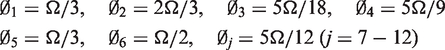$Ø_{2 i - 1} = Ω η_{i} ɛ_{2 i - 1}$ and $Ø_{2 i} = Ω η_{i} ɛ_{2 i}$ (i = 1–6) of the left and right segments of each main cable are

Ø_{1} = Ω / 3, Ø_{2} = 2 Ω / 3, Ø_{3} = 5 Ω / 18, Ø_{4} = 5 Ω / 9 Ø_{5} = Ω / 3, Ø_{6} = Ω / 2, Ø_{j} = 5 Ω / 12 (j = 7 - 12)

(27)

Based on Equation (15), the system characteristic equation of this example network can be expressed as

Denote $Ø_{1, 5} = Ø_{1} = Ø_{5},$ $Ø_{7, 9, 11} = Ø_{7} = Ø_{9} = Ø_{11},$ $Ø_{8, 10, 12} = Ø_{8} = Ø_{10} = Ø_{12},$ $γ_{4, 5, 6} = γ_{4} = γ_{5} = γ_{6}$ , and $η_{4, 5, 6} = η_{4} = η_{5} = η_{6}$ ; by rearranging the terms in Equation (27), it yields

\sin 2 (Ø_{1, 5}) \sin (Ø_{2}) \sin (Ø_{3}) \sin (Ø_{4}) \sin (Ø_{6}) \sin 3 (Ø_{7, 9, 11}) \sin 3 (Ø_{8, 10, 12}) {\frac{γ_{1} \sin (Ω η_{1})}{\sin (Ø_{1}) \sin (Ø_{2})} + \frac{γ_{2} \sin (Ω η_{2})}{\sin (Ø_{3}) \sin (Ø_{4})} + \frac{γ_{3} \sin (Ω η_{3})}{\sin (Ø_{5}) \sin (Ø_{6})} + 6 γ_{4, 5, 6} \frac{\cos (Ω η_{4, 5, 6} / 2)}{\sin (Ω η_{4, 5, 6} / 2)}} = 0

(28)

The roots of Equation (28) can be derived from the following conditions:

\frac{γ_{1} \sin (Ω η_{1})}{\sin (Ø_{1}) \sin (Ø_{2})} + \frac{γ_{2} \sin (Ω η_{2})}{\sin (Ø_{3}) \sin (Ø_{4})} + \frac{γ_{3} \sin (Ω η_{3})}{\sin (Ø_{5}) \sin (Ø_{6})} + 6 γ_{4, 5, 6} \frac{\cos (Ω η_{4, 5, 6} / 2)}{\sin (Ω η_{4, 5, 6} / 2)} = 0

(29a)

\sin (Ø_{2}) = 0 \sin 2 (Ø_{1, 5}) = 0

(29b, c)

\sin (Ø_{3}) = 0 \sin (Ø_{4}) = 0

(29d, e)

\sin (Ø_{6}) = 0 \sin (Ø_{7, 9, 11}) \sin (Ø_{8, 10, 12}) = 0

(29f, g)

\sin 2 (Ø_{7, 9, 11}) = 0 \sin 2 (Ø_{8, 10, 12}) = 0

(29h, i)

Among the above conditions, Equation (29a) describes the global modes of the network, whereas Equations (29b)–(29i) represent the local modes that involve oscillations of only certain cable(s) and/or cable segment(s). In particular, two sets of roots exist for Equations (29c), (29h), and (29i). The associated modes will be discussed later. The modal characteristics of the studied network can be obtained by plugging the numerical values of the system parameters into Equation (29). The modal frequencies of the first 14 modes and the corresponding mode shapes are portrayed in Figure 11.

Figure 11.

Modal characteristics of the first 14 modes of the example network.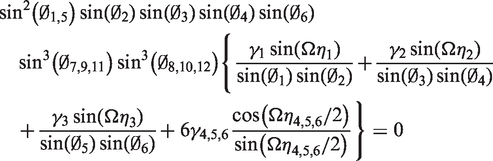

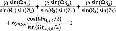
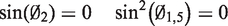
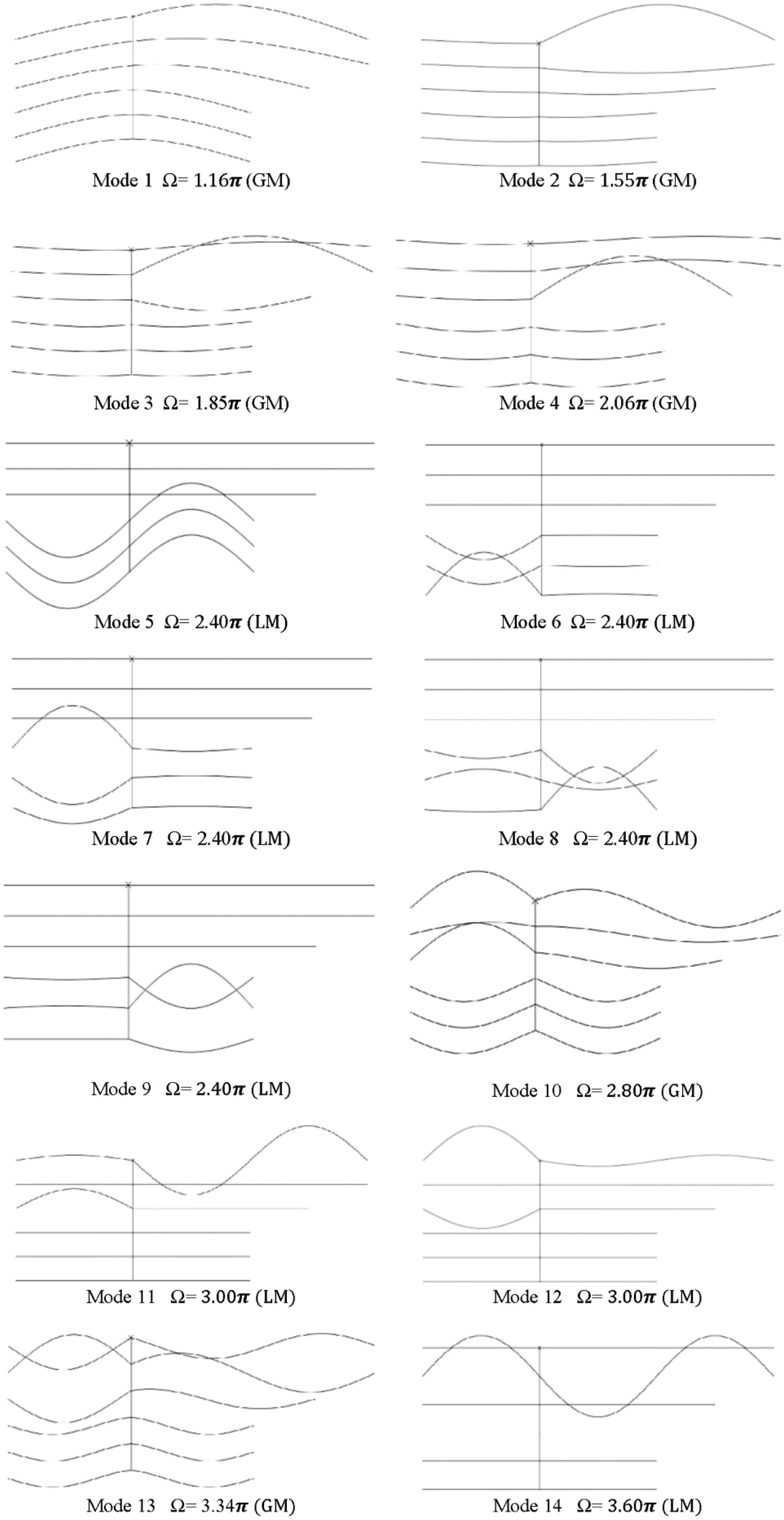
The first six roots of Equation (29a), in terms of the nondimensional system frequency Ω, are 1.16π, 1.55π, 1.85π, 2.06π, 2.80π, and 3.34π. They are the 1st, 2nd, 3rd, 4th, 10th, and 13th modes in Figure 11. In these modes, the left and the right segments of all six cables are excited to vibrate. Based on the definition of the nondimensional system frequency, that is, Ω = πf/f₁, where f and f₁ are respectively the network system frequency and the fundamental frequency of cable 1 (the target cable), by connecting the target cable with the other five cables in the current example, its fundamental frequency has been increased by 16%. It is interesting to note that in some of the global modes, certain cable segment(s) manifest(s) more significant oscillations than the others. This is mainly because the fundamental frequency of these segments happens to be in the vicinity of the global modes, and thus lead to ‘resonance’ phenomenon. For example, the frequency of mode 2 is Ω = 1.55π, whereas that of the right segment of cable 1, which yielded from $\sin (Ø_{2}) =$ sin( $2 Ω / 3) = 0,$ is Ω = 1.5π. Therefore, in mode 2, although all the cable segments are excited, the motion of the right segment in cable 1 takes dominance. Similarly, in the case of mode 3, since the frequencies of the right segment of cables 2 and 3 are 1.8π and 2.0π, respectively, they are close to the frequency Ω = 1.85π of this global mode. Thus, compared to the other parts of the network, these two-cable segments vibrate more sizably. The same reason can be used to explain why the right segment of cable 3 in mode 4 has more considerable oscillation than the rest part of the network. This cable segment has a fundamental frequency of 2.0π (yielded from $\sin (Ø_{6}) =$ sin( $Ω / 2) = 0$ ), which differs from the modal frequency Ω = 2.06π of mode 4 by only 2.9%.

The roots for Equation (29b) are Ω = 1.5nπ (n = 1, 2, 3…) which represent the local oscillations of the right segment of cable 1. The smallest root is Ω = 1.5π. Due to its close proximity with the second global mode frequency Ω = 1.55π, this local mode actually couples with the global mode in terms of more significant vibrations of this particular cable segment, as discussed earlier.

Equation (29c) has two sets of equal roots Ω = 3.0nπ (n = 1, 2, 3…). For each value of n, two modes with the same modal frequency but different mode shape are present. When n = 1, they represent modes 11 and 12 in Figure 11, of which the left segment of cables 1 and 3 are excited in the 1st symmetric mode. In addition, since Ω = 3.0π is the second root of Equation (29b), in modes 11 and 12, the right segment of cable 1 is also vibrating, but in the 1st anti-symmetric mode.

The roots and the corresponding modal characteristics associated with Equations (29d) and (29e) are very similar to that of Equations (29b) and (29c). The roots of Equation (29e) are Ω = 1.8nπ (n = 1, 2, 3…), which represent the local motions of the right segment in cable 2. The lowest mode has a frequency of 1.8π, which is very close to the frequency Ω = 1.85π of the 3rd global mode and thus couples with it. The second root Ω = 3.6π (when n = 2), which describes the oscillation of this cable segment in the 1st anti-symmetric mode, happens to be the smallest root of Equation (29d) representing vibrations of the left segment of cable 2 in the 1st symmetric mode. The motions of these two-cable segments are thus coupled in mode 14. As can be seen in Figure 11, in mode 14, only cable 2 is excited. Its left segment vibrates in the 1st symmetric mode and its right segments in the 1st anti-symmetric mode.

Ω = 2.0nπ (n = 1, 2, 3…) are the roots for Equation (29f). They are associated with local motions of the right segment in cable 3. As mentioned earlier, the lowest frequency of Ω = 2.0π is very close to that of the 4th global mode (Ω = 2.06π). Thus, the two modes are coupled, and more considerable oscillation of this particular cable segment can be clearly observed from the mode shape of mode 4.

Equations (29g), (29h), and (29i) describe the local motions associated with the cable segments in cables 4, 5, and 6. Equation (29h) gives two sets of local modes (Ω = 2.4nπ, n = 1, 2, 3…) associated with oscillations of the left segments in these three cables. When n = 1, they are modes 6 and 7 in Figure 11. Similarly, Equation (29i) gives two sets of local modes (Ω = 2.4nπ, n = 1, 2, 3…) containing vibrations of the right segments of these three cables. The lowest value of Ω = 2.4π corresponds to modes 8 and 9 in Figure 11. In the case of Equation (29f), although the same roots of Ω = 2.4nπ (n = 1, 2, 3…) can be derived, the corresponding mode shapes include motions of both segments in cables 4, 5, and 6. When take n = 1, it corresponds to mode 5 in Figure 11.

To validate the above analytical results, an independent finite element numerical simulation is conducted. Table 4 lists the modal analysis results of the first 14 modes obtained from the proposed analytical model and finite element simulation. A very good agreement between the two sets of results can be clearly seen from the table, which further verifies the validity of the proposed analytical model.

Table 4.

In-plane modal properties of an asymmetric different-mass-tension six-cable network with a single line of rigid cross-ties at one-third span.

Mode number	Modal frequencies (Hz)		Mode shapes
Mode number	Proposed analytical model	FEA	Mode shapes
1	1.4727	1.4727	GM, 1- Sym., in-phase
2	1.9656	1.9655	GM, Cable 1 RS dominate
3	2.3463	2.3460	GM, Cable 2, 3 RS dominate
4	2.6050	2.6044	GM, Cable 3 RS dominate
5	3.0410	3.0395	LM, Cables 4, 5, 6 dominate
6	3.0410	3.0395	LM, Cables 4, 5, 6 LS dominate
7	3.0410	3.0395	LM, Cables 4, 5, 6 LS dominate
8	3.0410	3.0395	LM, Cables 4, 5, 6 RS dominate
9	3.0410	3.0395	LM, Cables 4, 5, 6 RS dominate
10	3.5478	3.5458	GM, Cables 1, 3 LS dominate
11	3.8013	3.7994	LM, Cables 1, 3(LS) dominate
12	3.8013	3.7994	LM, Cables 1, 3 LS dominate
13	4.2413	4.2382	GM
14	4.5615	4.5587	LM, Cable 2 dominate

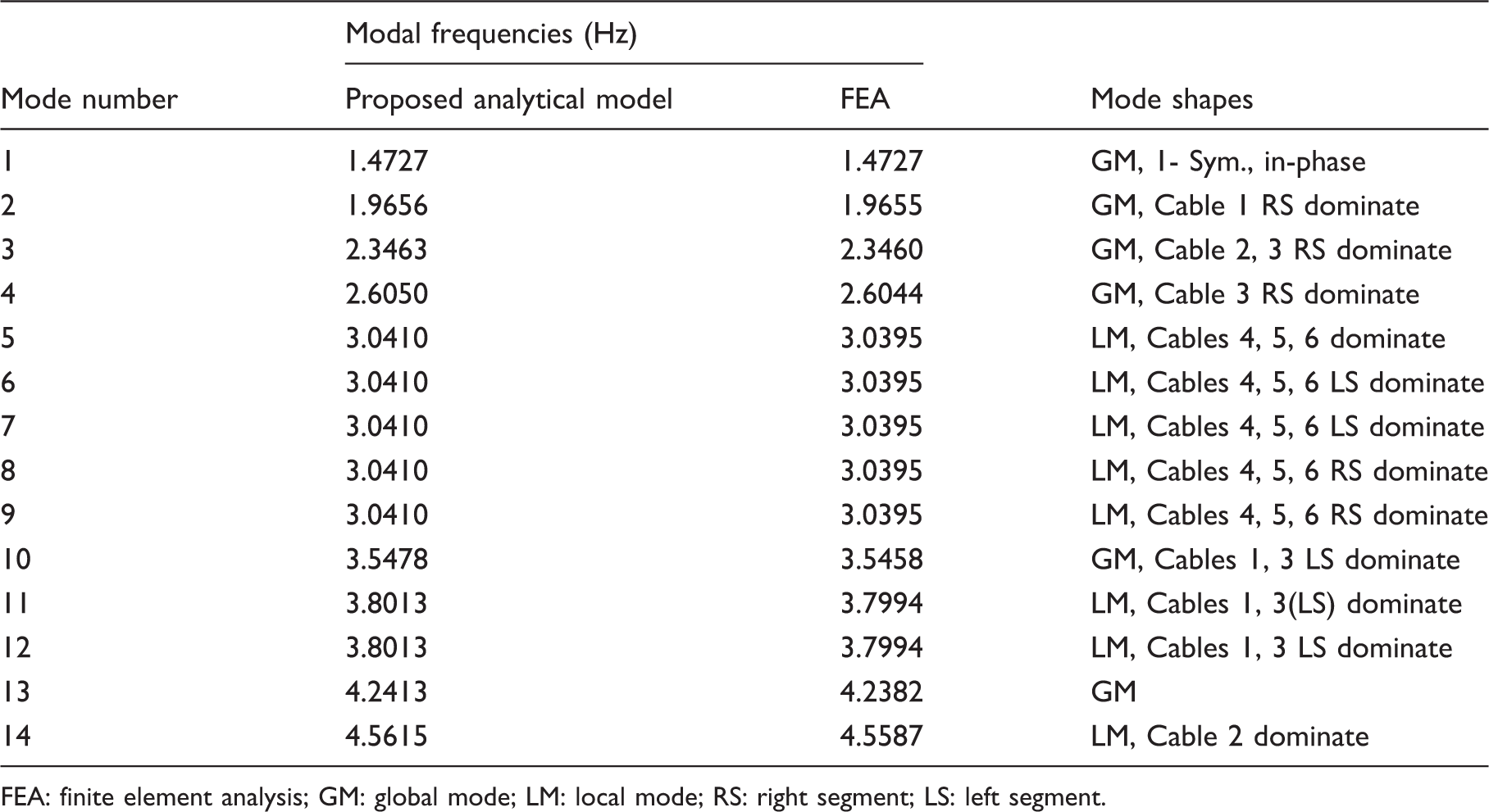
FEA: finite element analysis; GM: global mode; LM: local mode; RS: right segment; LS: left segment.

From the above discussion, it is clear that the local and the global modes are very sensitive to the frequency of different cable segments in a network. Under certain combinations of network geometric layout and cable properties, coupling between a local mode of cable segment(s) and a network global mode could occur, which is the ‘resonance’ phenomenon observed in the current example. This type of phenomenon should be avoided in the cable network design. When selecting the position for cross-ties, it is recommended that the so divided cable segments should not have local modal frequencies in the close proximity of the network global modal frequencies.

6. Conclusions

Using cross-ties is one of the effective countermeasures to suppress unfavorable bridge stay cable vibrations. Although the strategy has been successfully applied on site, the dynamic behavior of such a cable network is not fully understood. In this paper, an analytical model of a general cable network consisting of n horizontally laid taut cables interconnected by a single line of transverse rigid cross-ties has been proposed in order to study its in-plane modal behavior. The proposed analytical model has been applied to a number of cable networks with various configurations to verify its validity and demonstrate its flexibility. The modal analysis results yielded from the proposed analytical model are found to agree well with those obtained from an independent numerical simulation. The following conclusions can be drawn from the present work.

The segment ratio, the frequency ratio, the mass-tension ratio, and the number of main cables are identified to be the key system parameters that govern the in-plane modal behavior of a cable network with a single line of rigid transverse cross-ties.

In addition to the global modes, of which all main cables in the network are excited, numerous local modes dominated by a single main cable, or a group of few main cables, or part of the main cables (left or right segments) also exist in a cable network.

The modal properties of the global modes in a twin-cable network are independent of the segment ratio. However, the local modes, dominated by either the right or the left segments of the main cables, purely depend on this parameter. They form complimentary pairs. At certain cross-tie positions, a modal tri-furcation phenomenon, of which a pair of complimentary local modes coexist with either a symmetric or an asymmetric global mode, has been observed. A minor variation of the cross-tie position at the vicinity of these segment ratio values could cause a drastic change of the modal behavior.

Except the twin-cable system, in all the other studied cable network configurations, the modal frequencies of the global modes are higher than those of the target cable (main cable 1). Thus, the cross-tie solution is beneficial for enhancing the in-plane stiffness of the target cable.

To improve the in-plane stiffness of a target cable, it should be connected with neighboring cables having either lower frequency ratio and/or higher mass-tension ratio.

In a symmetric SMT four-cable network, when all three neighboring cables have the same frequency ratio and a single line of rigid cross-ties is installed at the mid-span, five different sets of local modes are identified to share the same modal frequency. These local modes are dominated by vibrations of either a single or a group of two neighboring main cables. This is consistent with the findings by Caracoglia and Zuo (2009), which suggested avoiding the evenly spaced configuration, since local modes associated with main cables cannot be suppressed.

The selection of cross-tie position should avoid inducing of modal frequency resonance between a global mode and local mode(s) of cable segment(s).

It is worth pointing out that using cross-tie(s) to connect a problematic cable with its neighbor(s) would not only affect its modal frequency, but also will have an impact on its damping property. Also, the impact of the identified key system parameters on the in-plane modal behavior of a general cable network need to be investigated in depth. The nonlinear interaction between the transverse vibration of main cables and the longitudinal motion of cross-ties has not been considered in the analytical formulation of the current work. However, as indicated by Giaccu and Caracoglia (2012, 2013), snapping or slacking of cross-ties may occur on real bridges, of which the cross-ties would exhibit nonlinear behavior. These issues will be further explored in future publications to comprehend our understanding of mechanics associated with a cable network system, which is expected to contribute to the more effective design of such a cable vibration control strategy. In addition, the current analytical study is focused on cable networks consisting of n horizontally laid main cables interconnected transversely with a single line of rigid cross-ties having idealized orthogonal configuration between main cables and cross-ties, and thus cannot be directly applied to cable networks on real bridges. However, it is very important to properly understand the mechanisms associated with such a more idealized system before introducing various other factors. Seeking an 'elegant' solution for practical cable networks having multiple cross-ties and inclined cables will be challenging. The effort made in the present work will serve as paving stones to lead us closer to this goal.

Footnotes

Funding

This work was supported by the Natural Sciences and Engineering Research Council of Canada (NSERC).

References

Ahmad

Cheng

(2013a) Impact of key system parameters on the in-plane dynamic response of a cable Network. Journal of Structural Engineering ASCE. Epub ahead of print 10 April 2013. Available at: DOI: 10.1061/(ASCE)ST.1943-541X.0000847.

Ahmad

Cheng

(2013b) Effect of cross-link stiffness on the in-plane free vibration behavior of a two-cable network. Engineering Structures 52: 570–580.

Bosch HR and Park SW (2005) Effectiveness of external dampers and crossties in mitigation of stay cable vibrations. In: proceedings of the 6th international symposium on cable dynamics, pp.115–122.

Caetano E and Cunha A (2003) Identification of parametric excitation at the International Guadiana Bridge. In: proceedings of the 5th international symposium on cable dynamics, pp.525-532.

Caracoglia

Jones

(2005a) In-plane dynamic behavior of cable networks. Part 1: Formulation and basic solutions. Journal of Sound and Vibration 279: 969–991.

Caracoglia

Jones

(2005b) In-plane dynamic behavior of cable networks. Part 2: Prototype prediction and validation. Journal of Sound and Vibration 279: 993–1014.

Caracoglia

Zuo

(2009) Effectiveness of cable networks of various configurations in suppressing stay-cable vibration. Engineering Structures 31: 2851–2864.

Cheng

Darivandi

Ghrib

(2010) The design of an optimal viscous damper for a bridge stay cable using energy-based approach. Journal of Sound and Vibration 329: 4689–4704.

Ehsan F and Scanlan RH (1989) Damping stay cables with ties. In: proceedings of the 5th US-Japan bridge workshop, pp.203-217.

10.

Fujino

Hoang

(2008) Design formulas for damping of a stay cable with a damper. Journal of Structural Engineering ASCE 134(2): 269–278.

11.

Giaccu

Caracoglia

(2012) Effects of modeling nonlinearity in cross-ties on the dynamics of simplified in-plane cable networks. Structural Control and Health Monitoring 19(3): 348–369.

12.

Giaccu

Caracoglia

(2013) Generalized power-law stiffness model for nonlinear dynamics of in-plane cable networks. Journal of Sound and Vibration 332(8): 1961–1981.

13.

Gimsing

Georgakis

(1993) Cable supported Bridges: Concept and Design, 3rd ed. New York: John Willy & Sons Ltd.

14.

Humar

(2002) Dynamics of Structures, 2nd ed. A.A. Rotterdam: Balkema Publishers.

15.

Irvine HM and Caughey TK (1974) The linear theory of free vibrations of a suspended cable. Proceedings of the Royal Society of London. Series A, Mathematical and Physical Sciences 341(1626): 299--315.

16.

Krenk

(2000) Vibrations of a taut cable with an external damper. Journal of Applied Mechanics 67(4): 772–776.

17.

Kumarasena S, Jones NP, Irwin P, et al. (2007) Wind-induced vibration of stay cables. FHWA-HRT-05-083. U.S. Department of Transportation, Federal Highway Administration.

18.

Lilien

Pinto da costa

(1994) Vibration amplitudes caused by parametric excitation of cable-stayed structures. Journal of Sound and Vibration 174(1): 69–90.

19.

Macdonald J and Georgakis CT (2002) The influence of cable-deck interaction on the seismic response of cable-stayed bridges. In: proceedings of the 12th European conference on earthquake engineering, Paper 441.

20.

Main

Jones

(2002) Free vibration of taut cable with attached damper, I: Linear Viscous Damper. Journal of Engineering Mechanics ASCE 128(10): 1062–1071.

21.

Matsumoto

Shirashi

Shirato

(1992) Rain-wind induced vibration of cables of cable-stayed bridges. Journal of Wind Engineering & Industrial Aerodynamics 43(1–3): 2011–2022.

22.

Pacheco

Fujino

Sulekh

(1993) Estimation curve for modal damping in stay cables with viscous damper. Journal of structural Engineering ASCE 119(6): 1961–1979.

23.

Sun

Wang

(2003) Parametrically excited oscillations of stay cable and its control in cable-stay bridges. Journal of Zhejiang University – Science A 4(1): 13–20.

24.

Sun L, Zhou Y and Huang H (2007) Experiment and damping evaluation on stay cables connected by cross ties. In: proceedings of the 7th international symposium on cable dynamics, Paper ID: 50.

25.

Tabatabai

Mehrabi

(2000) Design of mechanical viscous dampers for stay cables. Journal of Bridge Engineering ASCE 5(2): 114–123.

26.

Virlogeux

. Cable vibrations in cable-stayed bridges. In: Larsen

Esdahl

(eds). Bridge Aerodynamics, A A Balkema PublishersRotterdam, 1998, pp. 213–233.

27.

Yamaguchi

Nagahawatta

(1995) Damping effects of cable cross-ties in cable-stayed bridges. Journal of Wind Engineering & Industrial Aerodynamics 54/55: 35–43.

28.

Zhan

Zhou

(2008) Experimental study of wind–rain-induced cable vibration using a new model setup scheme. Journal of Wind Engineering & Industrial Aerodynamics 96(12): 2438–2451.

29.

Zhou H, Zhu Y, Yang Z, et al. (2011) Free vibration of taut cable with multiple spring supports. In: proceedings of the 9th international symposium on cable dynamics, pp.311–318.